Downloaded 243 times


![NOMENCLATURE
NOMENCLATURE xix
The dimensions for each symbol are represented in both the SI and English systems of
units, where applicable. Note that both the hour and second are commonly used as units
for time in the English system of units; hence a conversion factor of 3600 should be
employed at appropriate places in dimensionless groups.
A total heat transfer surface area (both primary and secondary, if any) on one
side of a direct transfer type exchanger (recuperator), total heat transfer
surface area of all matrices of a regenerator,{ m2, ft2
Ac total heat transfer area (both primary and secondary, if any) on the cold side
of an exchanger, m2, ft2
Aeff effective surface area on one side of an extended surface exchanger [defined by
Eq. (4.167)], m2, ft2
Af fin or extended surface area on one side of the exchanger, m2, ft2
Afr frontal or face area on one side of an exchanger, m2, ft2
Afr;t window area occupied by tubes, m2, ft2
Afr;w gross (total) window area, m2, ft2
Ah total heat transfer surface area (both primary and secondary, if any) on the
hot fluid side of an exchanger, m2, ft2
Ak fin cross-sectional area for heat conduction in Section 4.3 (Ak;o is Ak at the
fin base), m2, ft2
Ak total wall cross-sectional area for longitudinal conduction [additional
subscripts c, h, and t, if present, denote cold side, hot side, and total (hot þ
cold) for a regenerator] in Section 5.4, m2, ft2
A*k
ratio of Ak on the Cmin side to that on the Cmax side [see Eq. (5.117)],
dimensionless
Ao minimum free-flow (or open) area on one fluid side of an exchanger, heat
transfer surface area on tube outside in a tubular exchanger in Chapter 13
only, m2, ft2
Ao;bp flow bypass area of one baffle, m2, ft2
Ao;cr flow area at or near the shell centerline for one crossflow section in a shell-and-tube
exchanger, m2, ft2
Ao;sb shell-to-baffle leakage flow area, m2, ft2
Ao;tb tube-to-baffle leakage flow area, m2, ft2
Ao;w flow area through window zone, m2, ft2
Ap primary surface area on one side of an exchanger, m2, ft2
Aw total wall area for heat conduction from the hot fluid to the cold fluid, or total
wall area for transverse heat conduction (in the matrix wall thickness direc-tion),
m2, ft2
a short side (unless specified) of a rectangular cross section, m, ft
a amplitude of chevron plate corrugation (see Fig. 7.28), m, ft
{ Unless clearly specified, a regenerator in the nomenclature means either a rotary or a fixed-matrix regenerator.](https://image.slidesharecdn.com/fundamentalsofheatexchangerdesign-131001160835-phpapp01-141008073824-conversion-gate02/85/Fundamentalsofheatexchangerdesign-131001160835-phpapp01-18-320.jpg)
![xx NOMENCLATURE
B parameter for a thin fin with end leakage allowed, he=mkf , dimensionless
Bi Biot number, Bi ¼ hð=2Þ=kf for the fin analysis; Bi ¼ hð=2Þ=kw for the
regenerator analysis, dimensionless
b distance between two plates in a plate-fin heat exchanger [see Fig. 8.7 for b1
or b2 (b on fluid 1 or 2 side)], m, ft
b long side (unless specified) of a rectangular cross section, m, ft
c some arbitrary monetary unit (instead of $, £, etc.), money
C flow stream heat capacity rate with a subscript c or h, m_ cp, W=K, Btu/hr-8F
C correction factor when used with a subscript different from c, h, min, or max,
dimensionless
C unit cost, c/J(c/Btu), c/kg (c/lbm), c/kW [c/(Btu/hr)], c/kW yr(c/Btu on
yearly basis), c/m2(c/ft2)
C annual cost, c/yr
C* heat capacity rate ratio, Cmin=Cmax, dimensionless
C flow stream heat capacitance, Mcp, Cd, W s=K, Btu/8F
CD drag coefficient, p=ðu1=2
2gc
Þ, dimensionless
Cmax maximum of Cc and Ch, W=K, Btu/hr-8F
Cmin minimum of Cc and Ch, W/K, Btu/hr-8F
Cms heat capacity rate of the maldistributed stream, W/K, Btu/hr-8F
Cr heat capacity rate of a regenerator, MwcwN or Mwcw=Pt [see Eq. (5.7) for the
hot- and cold-side matrix heat capacity rates Cr;h and Cr;c], W/K, Btu/hr-8F
C*r
total matrix heat capacity rate ratio, Cr=Cmin, C*r
;h
¼ Cr;h=Ch, C*r
;c
¼ Cr;c=Cc,
dimensionless
Cr total matrix wall heat capacitance, Mwcw or CrPt [see Eq. (5.6) for hot- and
cold-side matrix heat capacitances Cr;h and Cr;c], W s=K, Btu/8F
C*r
ratio of Cr to Cmin, dimensionless
CUA cost per unit thermal size (see Fig. 10.13 and Appendix D), c/W/K
Cus heat capacity rate of the uniform stream, W/K, Btu/hr-8F
Cw matrix heat capacity rate; same as Cr, W/K, Btu/hr-8F
Cw total wall heat capacitance for a recuperator, Mwcw, W s=K, Btu/8F
Cw* ratio of Cw to Cmin, dimensionless
CF cleanliness factor, Uf =Uc, dimensionless
c specific heat of solid, J=kg K,{ Btu/lbm-8F
c annual cost of operation percentile, dimensionless
cp specific heat of fluid at constant pressure, J=kg K, Btu/lbm-8F
cw specific heat of wall material, J=kg K, Btu/lbm-8F
d exergy destruction rate, W, Btu/hr
Dbaffle baffle diameter, m, ft
Dctl diameter of the circle through the centers of the outermost tubes, Dotl
do,
m, ft
Dh hydraulic diameter of flow passages, 4rh, 4Ao=P, 4AoL=A, or 4=, m, ft
{ J ¼ joule ¼ newton meter ¼ watt second; newton ¼ N ¼ kg m=s2:](https://image.slidesharecdn.com/fundamentalsofheatexchangerdesign-131001160835-phpapp01-141008073824-conversion-gate02/85/Fundamentalsofheatexchangerdesign-131001160835-phpapp01-19-320.jpg)
![NOMENCLATURE xxi
Dh;w hydraulic diameter of the window section, m, ft
Dotl diameter of the outer tube limit (see Fig. 8.9), m, ft
Dp port or manifold diameter in a plate heat exchanger, m, ft
Ds shell inside diameter, m, ft
d differential operator
dc collar diameter in a round tube and fin exchanger, do
þ 2, m, ft
de fin tip diameter of a disk (radial) fin, m, ft
di tube inside diameter, m, ft
do tube (or pin) outside diameter, tube outside diameter at the fin root for a
finned tube after tube expansion, if any, m, ft
dw wire diameter, m, ft
d1 tube hole diameter in a baffle, m, ft
_e
e exergy rate, W, Btu/hr
E energy, J, Btu
E activation energy in Chapter 13 [see Eq. (13.12)], J=kg mol, Btu/lbm-mole
E fluid pumping power per unit surface area, m_ p=A, W=m2, hp/ft2
Eu row average Euler number per tube row, p=ðu2
mNr=2gc
Þ or
p=ðG2Nr=2gcÞ, dimensionless
e surface roughness size, m, ft
þ
e
roughness Reynolds number, eu*=, dimensionless
F log-mean temperature difference correction factor [defined by Eq. (3.183)],
dimensionless
f Fanning friction factor, w=ðu2
m=2gc
Þ, p gcDh=ð2LG2Þ, dimensionless
fD Darcy friction factor, 4f, dimensionless
ftb row average Fanning friction factor per tube for crossflow to tubes, used in
Chapter 7, p=ð4G2Nr=2gc Þ, Eu/4, dimensionless
G fluid mass velocity based on the minimum free area, m_ =Ao (replace Ao by Ao;c
for the crossflow section of a tube bundle in a shell-and-tube heat exchan-ger),
kg=m2 s, lbm/hr-ft2
Gr Grashof number [defined by Eq. (7.159)], dimensionless
Gz Graetz number, m_ cp=kL [see Eqs. (7.39) and (12.53)], dimensionless
Gzx local Graetz number, m_ cp=kx, dimensionless
g gravitational acceleration, m/s2, ft/sec2
gc proportionality constant in Newton’s second law of motion, gc
¼ 1 and
dimensionless in SI units, gc
¼ 32:174 lbm-ft/lbf-sec2
H head or velocity head, m, ft
H fluid enthalpy, J, Btu
_H
H enthalpy rate, used in Chapter 11, W, Btu/hr
Hg Hagen number, defined by Eq. (7.23), dimensionless
*H thermal boundary condition referring to constant axial as well as peripheral
wall heat flux; also constant peripheral wall temperature; boundary
condition valid only for the circular tube, parallel plates, and concentric
annular ducts when symmetrically heated](https://image.slidesharecdn.com/fundamentalsofheatexchangerdesign-131001160835-phpapp01-141008073824-conversion-gate02/85/Fundamentalsofheatexchangerdesign-131001160835-phpapp01-20-320.jpg)
![xxii NOMENCLATURE
*H1 thermal boundary condition referring to constant axial wall heat flux with
constant peripheral wall temperature
*H2 thermal boundary condition referring to constant axial wall heat flux with
constant peripheral wall heat flux
h heat transfer coefficient [defined by Eqs. (7.11) and (7.12)], W=m2 K, Btu/
hr-ft2-8F
h specific enthalpy, J/kg, Btu/lbm
he heat transfer coefficient at the fin tip, W=m2 K, Btu/hr-ft2-8F
h‘g specific enthalpy of phase change, J/kg, Btu/lbm
I_irr irreversibility rate (defined in Table 11.3), W, Btu/hr
In
ðÞ modified Bessel function of the first kind and nth order
ij flow direction indicator, ij
¼ þ1 or 1, fluid j ¼ 1 or 2, dimensionless
J mechanical to thermal energy conversion factor, J ¼ 1 and dimensionless in SI
units, J ¼ 778:163 lbf-ft/Btu
Ji correction factors for the shell-side heat transfer coefficient for the Bell–
Delaware method [see Eq. (9.50)]; i ¼ c for baffle cut and spacing; i ¼ ‘ for
baffle leakage effects, including both shell-to-baffle and tube-to-baffle leak-age;
i ¼ b for the bundle bypass flow (C and F streams); i ¼ s for variable
baffle spacing in the inlet and outlet sections; i ¼ r for adverse temperature
gradient buildup in laminar flow, dimensionless
j Colburn factor, St Pr2/3, ðh=Gcp
ÞPr2=3, dimensionless
K pressure loss coefficient, p=ðu2
m=2gc
Þ; subscripts: b for a circular bend, s for
a miter bend, and v for a screwed valve in Chapter 6, and br for branches in
Chapter 12, dimensionless
Kð1Þ incremental pressure drop number for fully developed flow (see Table 7.2 for
the definition), dimensionless
Kc contraction loss coefficient for flow at heat exchanger entrance, dimensionless
Ke expansion loss coefficient for flow at heat exchanger exit, dimensionless
Kn
ðÞ modified Bessel function of the second kind and nth order
k fluid thermal conductivity for fluid if no subscript, W=m K, Btu/hr-ft-8F
kf thermal conductivity of the fin material in Chapter 4 and of the foulant
material in Chapter 13, W=m K, Btu/hr-ft-8F
kw thermal conductivity of the matrix (wall) material, W=m K, Btu/hr-ft-8F
L fluid flow (core) length on one side of an exchanger, m, ft
Lf fin flow length on one side of a heat exchanger, Lf
L, m, ft
Lh plate length in a PHE for heat transfer (defined in Fig. 7.28), m, ft
Lp plate length in a PHE for pressure drop (defined in Fig. 7.28), m, ft
L1 flow (core) length for fluid 1 of a two-fluid heat exchanger, m, ft
L2 flow (core) length for fluid 2 of a two-fluid heat exchanger, m, ft
L3 noflow height (stack height) of a two-fluid heat exchanger, m, ft
Lq Le´veˆque number, defined by Eq. (7.41), dimensionless](https://image.slidesharecdn.com/fundamentalsofheatexchangerdesign-131001160835-phpapp01-141008073824-conversion-gate02/85/Fundamentalsofheatexchangerdesign-131001160835-phpapp01-21-320.jpg)
![NOMENCLATURE xxiii
‘ fin height or fin length for heat conduction from primary surface to either fin
tip or midpoint between plates for symmetric heating, ‘ ¼ ðde
do
Þ=2 for
individually finned tubes, ‘ with this meaning used only in the fin analysis
and in the definition of f, m, ft
‘c baffle cut, distance from the baffle tip to the shell inside diameter (see Fig. 8.9),
m, ft
‘ef effective flow length between major boundary layer disturbances, distance
between interruptions, m, ft
‘s strip length of an offset strip fin, m, ft
‘* flow length between interruptions, ‘ef=ðDh
Re PrÞ, dimensionless
‘c* baffle cut, ‘c=Ds, dimensionless
m molecular weight (molar mass) of a gas, kg/kmol, lbm/lb mole
MA foulant material mass per unit heat transfer surface area in Chapter 13, m/A,
kg/m2, lbm/ft2
Mw mass of a heat exchanger core or the total mass of all matrices of a regenerator,
kg, lbm
m fin parameter [defined by Eqs. (4.62) and (4.65); see also Table 4.5 for other
definitions], 1/m, 1/ft
m mass of a body or fluid in a control volume, kg, lbm
m_ fluid mass flow rate, umAo, kg/s, 1bm/hr
m_ n fluid mass flow rate for nominal flow passages in Chapter 12, kg/s, 1bm/hr
N number of subexchangers in gross flow maldistributed exchanger or a number
of differently sized/shaped passages in passage-to-passage nonuniformity,
used in Chapter 12
N rotational speed for a rotary regenerator, rev/s, rpm
Nb number of baffles in a plate-baffled shell-and-tube exchanger
Nc number of fluid channels in a plate heat exchanger
Nf number of fins per unit length in the fin pitch direction, l/m, l/ft
Np number of fluid 1 passages in a two-fluid heat exchanger
Np number of pass divider lanes through the tube field that are parallel to the
crossflow stream in a shell-and-tube exchanger
N
0
p number of separating plates in a plate-fin exchanger, number of pass divider
lanes in a shell-and-tube exchanger
Nr number of tube rows in the flow direction
Nr;c number of effective tube rows crossed during flow through one baffle section,
Nr;cc
þ Nr;cw
Nr;cc number of effective tube rows crossed during flow through one crossflow
section (between baffle tips)
Nr;cw number of effective tube rows crossed during flow through one window zone in
a segmental baffled shell-and-tube heat exchanger
Nt total number of tubes in an exchanger, total number of holes in a tubesheet, or
total number of plates in a plate heat exchanger
Nt;b total number of tubes associated with one segmental baffle](https://image.slidesharecdn.com/fundamentalsofheatexchangerdesign-131001160835-phpapp01-141008073824-conversion-gate02/85/Fundamentalsofheatexchangerdesign-131001160835-phpapp01-22-320.jpg)
![xxiv NOMENCLATURE
Nt;c number of tubes at the tube bundle centerline cross section
Nt; p number of tubes per pass
Nt;w number of tubes in the window zone
N
0
t number of tubes in a specified row
NTU number of exchanger heat transfer units, UA=Cmin [defined by Eqs. (3.59)
through (3.64)], it represents the total number of transfer units in a multipass
unit, dimensionless
NTU1 number of exchanger heat transfer units based on fluid 1 heat capacity rate,
UA=C1; similarly, NTU2
¼ UA=C2, dimensionless
NTUc number of exchanger heat transfer units based on Cc, UA=Cc, dimensionless
NTUh number of exchanger heat transfer units based on Ch, UA=Ch, dimensionless
NTUo modified number of heat transfer units for a regenerator [defined by Eq.
(5.48)], dimensionless
NTU* number of heat transfer units at maximum entropy generation, dimensionless
Nu Nusselt number [defined by Eqs. (7.26) and (7.27)], dimensionless
n, np number of passes in an exchanger
nc number of cells of a regenerator matrix per unit of frontal area, 1/m2, 1/ft2
nf total number of fins on one fluid side of an extended-surface exchanger
nt number of tubes in each pass
ntuc number of heat transfer units based on the cold fluid side, ðohAÞ
c=Cc,
dimensionless
ntu*cost reduction in ntu [defined by Eq. (12.44)], dimensionless
ntuh number of heat transfer units based on the hot fluid side, ðohAÞ
h=Ch,
dimensionless
P fluid pumping power, m_ p=, W, hp
P temperature effectiveness for one fluid stream [defined by Eqs. (3.96) and
(3.97)], dimensionless
P wetted perimeter of exchanger passages on one fluid side, P ¼ A=L ¼
Afr, m, ft
} deposition probability function, dimensionless
Pc cold-gas flow period, duration of the cold-gas stream in the matrix or duration
of matrix in the cold-gas stream, used in Chapter 5, s, sec
Ph hot-gas flow period, duration of the hot-gas stream in the matrix or duration
of matrix in the hot-gas stream, used in Chapter 5, s, sec
Pr reversal period for switching from hot- to cold-gas stream, or vice versa, in a
fixed-matrix regenerator, used in Chapter 5, s, sec
Pt total period between the start of two successive heating (or cooling) periods in
a regenerator, used in Chapter 5, Pt
¼ Ph
þ Pc
þ Pr
Ph
þ Pc, s, sec
Pe Pe´ clet number, Re Pr, dimensionless
Pr Prandtl number, cp=k, umDh=, dimensionless
p fluid static pressure, Pa, lbf/ft2 (psf ) or lbf/in2 (psi){
{ Pa ¼ Pascal ¼ N=m2 ¼ kg=m s2; N ¼ newton ¼ kg m=s2; psf ¼ lbf=ft3; psi ¼ lbf=in3:](https://image.slidesharecdn.com/fundamentalsofheatexchangerdesign-131001160835-phpapp01-141008073824-conversion-gate02/85/Fundamentalsofheatexchangerdesign-131001160835-phpapp01-23-320.jpg)
![NOMENCLATURE xxv
p porosity of a matrix, a ratio of void volume to total volume of a matrix, rh,
dimensionless
p* ratio of cold-fluid inlet pressure to hot-fluid inlet pressure, pc;i=ph;i , dimension-less
pd fin pattern depth, peak-to-valley distance, excluding fin thickness (see Fig.
7.30), m, ft
pf fin pitch, 1=Nf, m, ft
pt tube pitch, center-to-center distance between tubes, m, ft
p fluid static pressure drop on one fluid side of a heat exchanger core [see
Eq. (6.28)], Pa, psf (psi)
p* ¼ p=ðu2
m=2gc
Þ, dimensionless
pb fluid static pressure drop associated with a pipe bend, Pa, psf (psi)
pb;i fluid static pressure drop associated with an ideal crossflow section between
two baffles, Pa, psf (psi)
pc fluid static pressure drop associated with the tube bundle central section
(crossflow zone) between baffle tips, Pa, psf (psi)
pgain pressure drop reduction due to passage-to-passage nonuniformity [defined by
Eq. (12.36)], Pa, psf (psi)
ps shell-side pressure drop, Pa, psf (psi)
pw;i fluid static pressure drop associated with an ideal window section, Pa, psf (psi)
Q heat transfer in a specified period or time, J, Btu
q total or local (whatever appropriate) heat transfer rate in an exchanger, or
heat ‘‘duty,’’ W, Btu/hr
q* normalized heat transfer rate, q=½ðm_ cp
ÞðT2;i
T1;i
Þ, dimensionless
q
0
heat transfer rate per unit length, q=L, W/m, Btu/hr-ft
q
00
heat flux, heat transfer rate per unit surface area, q=A, W/m2, Btu/hr-ft2
qe heat transfer rate through the fin tip, W, Btu/hr
q0 heat transfer rate at the fin base, W, Btu/hr
qmax thermodynamically maximum possible heat transfer rate in a counterflow heat
exchanger as expressed by Eq. (3.42), and also that through the fin base as
expressed by Eq. (4.130), W, Btu/hr
R universal gas constant, 8.3143 kJ=kmol K, 1545.33 1bf-ft/1b mole-8R
R heat capacity rate ratio [defined by Eqs. (3.105) and (3.106)], dimensionless
R thermal resistance based on the surface area A; R ¼ 1=UA ¼ overall thermal
resistance in a two-fluid exchanger, Rh
¼ 1=ðhAÞ
h
¼ hot-side film resistance
(between the fluid and the wall), Rc
¼ cold-side film resistance, Rf
¼ fouling
resistance, and Rw
¼ wall thermal resistance [definitions found after Eq.
(3.24)], K/W, hr-8F/Btu
^R
R ¼ RA ¼ 1=U, ^R
R unit thermal resistance, ^R
Rh
¼ 1=ðohÞ
h, ^R
Rw
¼ 1=ðohÞ
c,
^RRw
¼ w=Aw, m2 K=W, hr-ft2 8F/Btu
R* ratio of thermal resistances on the Cmin to Cmax side, 1=ðohAÞ*; it is also the
same as the ratio of hot to cold reduced periods, h=c, Chapter 5, dimen-sionless](https://image.slidesharecdn.com/fundamentalsofheatexchangerdesign-131001160835-phpapp01-141008073824-conversion-gate02/85/Fundamentalsofheatexchangerdesign-131001160835-phpapp01-24-320.jpg)
![xxvi NOMENCLATURE
R* total thermal resistance (wall, fouling, and convective) on the enhanced (or
plain with subscript p) ‘‘outside’’ surface side normalized with respect to the
thermal resistance ½1=ðhAi; Þ p
of ‘‘inside’’ plain tube/surface (see Table 10.5
for explicit formulas), dimensionless
~ R gas constant for a particular gas, R/m, J=kg K, 1bf-ft=1bm-8R
^R
Rf fouling factor or unit thermal resistance (‘‘fouling resistance’’), 1=hf ,
m2 K=W, hr-ft2-8F/Btu
Ri pressure drop correction factor for the Bell–Delaware method, where i ¼ b for
bundle bypass flow effects (C stream), i ¼ ‘ for baffle leakage effects (A and
E streams), i ¼ s for unequal inlet/outlet baffle spacing effects, dimension-less
Ra Rayleigh number [defined by Eq. (7.160)], dimensionless
Re Reynolds number based on the hydraulic diameter, GDh= , dimensionless
Red Reynolds number based on the tube outside diameter and mean velocity,
um do= , dimensionless
Redc Reynolds number based on the collar diameter and mean velocity, um dc= ,
dimensionless
Reo Reynolds number based on the tube outside diameter and free stream
(approach or core upstream) velocity, u1 do= , dimensionless
^r radial R
coordinate in the cylindrical coordinate system, m, ft
rc radius of curvature of a tube bend (see Fig. 6.5), m, ft
rf fouling factor or fouling resistance rf
¼ Rf
¼ 1=hf
¼ f =kf, m2 K=W, hr-ft2-
8F/Btu
rh hydraulic radius, AoL=A or Dh=4, m, ft
ri tube inside radius, m, ft
S entropy, J/K, Btu/8R
S* normalized entropy generation rate, _S
Sirr=C2 or _SSirr=Cmax, dimensionless
_S
Sirr entropy generation rate, W/K, Btu/hr-8R
St Stanton number, h=Gcp, Sto
¼ U=Gcp, dimensionless
s specific entropy in Chapter 11, J=kg K, Btu/lbm-8R
s complex Laplace independent variable with Laplace transforms only in
Chapter 11, dimensionless
s spacing between adjacent fins, pf
, m, ft
T fluid static temperature to a specified arbitrary datum, except for Eqs. (7.157)
and (7.158) and in Chapter 11 where it is defined on an absolute temperature
scale, 8C, 8F
*T thermal boundary condition referring to constant wall temperature, both
axially and peripherally
Tc;o flow area average cold-fluid outlet temperature unless otherwise specified, 8C,
8F
Th;o flow area average hot-fluid outlet temperature unless otherwise specified, 8C,
8F
T‘ temperature of the fin tip, 8C, 8F
Tm fluid bulk mean temperature, 8C, 8F](https://image.slidesharecdn.com/fundamentalsofheatexchangerdesign-131001160835-phpapp01-141008073824-conversion-gate02/85/Fundamentalsofheatexchangerdesign-131001160835-phpapp01-25-320.jpg)
![NOMENCLATURE xxvii
Ts steam temperature, 8C, 8F
Tw wall temperature, 8C, 8F
T1 ambient fluid temperature, free stream temperature beyond the extent of the
boundary layer on the wall, 8C, 8F
T* ratio of hot-fluid inlet temperature to cold-fluid inlet temperature, Th;i=Tc;i ,
dimensionless
Tc* ¼ ðTc
Tc;i
Þ=ðTh;i
Tc:i
Þ, dimensionless
Th* ¼ ðTh
Tc;i
Þ=ðTh;i
Tc:i
Þ, dimensionless
Tw* ¼ ðTw
Tc;i
Þ=ðTh;i
Tc;i
Þ, dimensionless
T0 temperature of the fin base, 8C, 8F
T local temperature difference between two fluids, Th
Tc, 8C, 8F
Tc temperature rise of the cold fluid in the exchanger, Tc;o
Tc;i , 8C, 8F
Th temperature drop of the hot fluid in the exchanger, Th;i
Th;o, 8C, 8F
Tlm log-mean temperature difference [defined by Eq. (3.172)], 8C, 8F
Tm true (effective) mean temperature difference [defined by Eqs. (3.9) and (3.13)],
8C, 8F
Tmax inlet temperature difference (ITD) of the two fluids, ðTh;i
Tc;i
Þ, ðTw;i
Ta;i
Þ
in Section 7.3.1, 8C, 8F
U, Um overall heat transfer coefficient [defined by Eq. (3.20) or (3.24)], subscript
m represents mean value when local U is variable (see Table 4.2 for the
definitions of other U’s), W=m2 K, Btu/hr-ft2-8F
u, um fluid mean axial velocity, um occurs at the minimum free flow area in the
exchanger unless specified, m/s, ft/sec
uc fluid mean velocity for flow normal to a tube bank based on the flow area of
the gap ðXt
do
Þ; evaluated at or near the shell centerline for a plate-baffled
shell-and-tube exchanger, m/s, ft/sec
ucr critical gap velocity for fluidelastic excitation or critical axial velocity for
turbulent buffeting, m/s, ft/sec
uz, uw effective and ideal mean velocities in the window zone of a plate-baffled shell-and-
tube exchanger [see Eq. (6.41)], m/s, ft/sec
u1 free stream (approach) velocity, m/s, ft/sec
u* friction velocity, ðwgc=Þ1=2, m/s, ft/sec
V heat exchanger total volume, Vh
¼ volume occupied by the hot-fluid-side heat
transfer surface area, Vc defined similarly for the cold fluid side, m3, ft3
V* ratio of the header volume to the matrix total volume, dimensionless
_V
V ¼ m_ = ¼ umAo, m3/s, ft3/sec
V volumetric flow rate, _V
Vm matrix or core volume, m3, ft3
Vp heat exchanger volume between plates on one fluid side, m3, ft3
Vv void volume of a regenerator, m3, ft3
v specific volume, 1=, m3=kg, ft3/1bm
W plate width between gaskets (see Fig. 7.28), m, ft
wp width of the bypass lane (see Fig. 8.9), m, ft
X* axial distance or coordinate, x=L, dimensionless](https://image.slidesharecdn.com/fundamentalsofheatexchangerdesign-131001160835-phpapp01-141008073824-conversion-gate02/85/Fundamentalsofheatexchangerdesign-131001160835-phpapp01-26-320.jpg)
![xxviii NOMENCLATURE
Xd diagonal pitch, ðX2
t
þ X2
‘
Þ1=2, m, ft
Xd* ratio of the diagonal pitch to the tube outside diameter in a circular tube bank,
Xd=do, dimensionless
X‘ longitudinal (parallel to the flow) tube pitch (see Table 8.1), m, ft
X‘* ratio of the longitudinal pitch to the tube outside diameter in a circular tube
bank, X‘=do, dimensionless
Xt transverse (perpendicular to the flow) tube pitch, m, ft
Xt* ratio of the transverse pitch to the tube diameter in a circular tube bank, Xt=do,
dimensionless
x Cartesian coordinate along the flow direction, m, ft
þ
x
axial distance, x=Dh
Re, dimensionless
x* axial distance, x=Dh
Re Pr, dimensionless
xf projected wavy length for one-half wavelength (see Fig. 7.30), m, ft
y transverse Cartesian coordinate, along the matrix wall thickness direction in a
regenerator, or along fluid 2 flow direction in other exchangers, m, ft
Z capital investment or operating expenses in Chapter 11, c/yr
z Cartesian coordinate, along the noflow or stack height direction for a plate-fin
exchanger, m, ft
fluid thermal diffusivity, k=cp, m2/s, ft2/sec
ratio of total heat transfer area on one fluid side of an exchanger to the total
volume of an exchanger, A=V, m2/m3, ft2/ft3
w thermal diffusivity of the matrix material, kw=wcw, m2/s, ft2/sec
* aspect ratio of rectangular ducts, ratio of the small to large side length,
dimensionless
f* fin aspect ratio, 2‘=, dimensionless
chevron angle for a PHE chevron plate measured from the axis parallel to the
plate length ( 908) (see Fig. 1.18c or 7.28), rad, deg
heat transfer surface area density: ratio of total transfer area on one fluid side
of a plate-fin heat exchanger to the volume between the plates on that fluid
side, A=AfrL, packing density for a regenerator, m2=m3, ft2=ft3
* coefficient of thermal expansion, 1=T for a perfect gas, 1/K, 1/8R
unbalance factor, ðc=Þ=ðc
h=h
Þ or Cc=Ch in Chapter 5 [see Eq. (5.92)],
dimensionless
specific heat ratio, cp=cv, dimensionless
denotes finite difference
@, partial and finite differential operators
fin thickness, at the root if the fin is not of constant cross section, m, ft
b segmental baffle thickness, m, ft
bb shell-to-tube bundle diametral clearance, Ds
Dotl, m, ft
c channel deviation parameter [defined in Eqs. (12.44), (12.46), and (12.47)],
dimensionless
f fouling film thickness, m, ft
h header thickness, m, ft](https://image.slidesharecdn.com/fundamentalsofheatexchangerdesign-131001160835-phpapp01-141008073824-conversion-gate02/85/Fundamentalsofheatexchangerdesign-131001160835-phpapp01-27-320.jpg)
![NOMENCLATURE xxix
‘ laminar (viscous) sublayer thickness in a turbulent boundary layer, m, ft
otl shell-to-tube outer limit diameter clearance, Do
Dotl, m, ft
s leakage and bypass stream correction factor to the true mean temperature
difference for the stream analysis method [defined by Eq. (4.170)], dimen-sionless
sb shell-to-baffle diametral clearance, Ds
Dbaffle, m, ft
tb tube-to-baffle hole diametral clearance, d1
do, m, ft
t thermal boundary layer thickness, m, ft
v velocity boundary layer thickness, m, ft
w wall or primary surface (plate) thickness, m, ft
heat exchanger effectiveness [defined by Eq. (3.37) or (3.44) and Table 11.1];
represents an overall exchanger effectiveness for a multipass unit, dimen-sionless
c temperature effectiveness of the cold fluid [defined by Eq. (3.52)], also as the
exchanger effectiveness of the cold fluid in Appendix B, dimensionless
cf counterflow heat exchanger effectiveness [see Eq. (3.83)], dimensionless
h temperature effectiveness of the hot fluid [defined by Eq. (3.51)], also as the
exchange effectiveness of the hot fluid in Appendix B, dimensionless
h;o temperature effectiveness of the hot fluid when flow is uniform on both fluid
sides of a two-fluid heat exchanger (defined the same as h), dimensionless
p heat exchanger effectiveness per pass, dimensionless
r regenerator effectiveness of a single matrix [defined by Eq. (5.81)], dimension-less
* effectiveness deterioration factor, dimensionless
Cartesian coordinate, ðy=L2
ÞC* NTU [see Eq. (11.21)], dimensionless
i correction factors for shellside pressure drop terms for the Bell–Delaware
method [see Eq. (9.51)]; i ¼ ‘ for tube-to-baffle and baffle-to-shell leakage;
i ¼ b for bypass flow; i ¼ s for inlet and outlet sections, dimensionless
reduced time variable for a regenerator [defined by Eq. (5.69)] with subscripts
j ¼ c and h for cold- and hot-gas flow periods, dimensionless
exergy efficiency [defined by Eq. (11.60)], dimensionless
f fin efficiency [defined by Eq. (4.129)], dimensionless
o extended surface efficiency on one fluid side of the extended surface heat
exchanger [see Eqs. (4.158) and (4.160) for the definition], dimensionless
ðohAÞ* convection conductance ratio [defined by Eq. (4.8)], dimensionless
p pump/fan efficiency, dimensionless
fin effectiveness [defined by Eq. (4.156)], dimensionless
¼ 1](https://image.slidesharecdn.com/fundamentalsofheatexchangerdesign-131001160835-phpapp01-141008073824-conversion-gate02/85/Fundamentalsofheatexchangerdesign-131001160835-phpapp01-28-320.jpg)


![excess temperature for the fin analysis in Chapter 4 [defined by Eq. (4.63)];](https://image.slidesharecdn.com/fundamentalsofheatexchangerdesign-131001160835-phpapp01-141008073824-conversion-gate02/85/Fundamentalsofheatexchangerdesign-131001160835-phpapp01-31-320.jpg)


![¼ ¼ r
2
3608, rad, deg
# fluid temperature for internal flow in Chapter 7, ðT Tw;m
Þ=ðTm
Tw;m
Þ,
dimensionless
# ratio of fluid inlet temperatures, T1;i=T2;i in Chapter 11 where temperatures
are on absolute temperature scale, dimensionless
#* fluid temperature for external flow, ðT Tw
Þ=ðT1 Tw
Þ or
ðT Tw
Þ=ðTe
Tw
Þ, dimensionless
length effect correction factor for the overall heat transfer coefficient [see Eqs.
(4.32) and (4.33)] dimensionless
T isothermal compressibility, 1/Pa, ft2/lbf
reduced length for a regenerator [defined by Eqs. (5.84), (5.102), and (5.103)],
dimensionless
m mean reduced length [defined by Eq. (5.91)], dimensionless
* ¼ h=c, dimensionless
, wavelength of chevron plate corrugation (see Fig. 7.28), m, ft
longitudinal wall conduction parameter based on the total conduction area,
¼ kwAk;t=CminL, c
¼ kwAk;c=CcLc, h
¼ kwAw;h=ChLh, dimensionless
fluid dynamic viscosity, Pa s, 1bm/hr-ft
fluid kinematic viscosity =, m2/s, ft2/sec
reduced length variable for regenerator [defined by Eq. (5.69], dimensionless
axial coordinate in Chapter 11, x=L, dimensionless
reduced period for a regenerator [defined by Eqs. (5.84), (5.104), and (5.105)],
dimensionless
m harmonic mean reduced period [defined by Eq. 5.90)], dimensionless
fluid density, kg/m3, 1bm/ft3
ratio of free flow area to frontal area, Ao=Afr, dimensionless
time, s, sec
d delay period or induction period associated with initiation of fouling in
Chapter 13; dwell time, residence time, or transit time of a fluid particle in a
heat exchanger in Chapter 5, s, sec
d;min dwell time of the Cmin fluid, s, sec
s fluid shear stress, Pa, psf
w equivalent fluid shear stress at wall, Pa, psf (psi)
* time variable, =d;min, dimensionless
*, * chtime variable for the cold and hot fluids [defined by Eq. (5.26)], dimensionless
ðÞ denotes a functional relationship
axial coordinate, ðx=L1
ÞNTU, in Chapter 11 only, dimensionless
xxx NOMENCLATURE](https://image.slidesharecdn.com/fundamentalsofheatexchangerdesign-131001160835-phpapp01-141008073824-conversion-gate02/85/Fundamentalsofheatexchangerdesign-131001160835-phpapp01-43-320.jpg)
![i fractional distribution of the ith shaped passage, dimensionless
Tm=ðTh;i
Tc;i
Þ, dimensionless
removal resistance [scale strength factor; see Eq. (13.12)], dimensionless
water quality factor, dimensionless
Subscripts
A unit (row, section) A
a air side
B unit (row, section) B
b bend, tube bundle, or lateral branch
c cold-fluid side, clean surface in Chapter 13
cf counterflow
cp constant properties
cr crossflow section in a segmental baffled exchanger
cv control volume
cu cold utility
d deposit
df displaced fluid
eff effective
f fouling, fluid in Section 7.3.3.2
g gas side
H constant axial wall heat flux boundary condition
h hot-fluid side
hu hot utility
hex heat exchanger
H1 thermal boundary condition referring to constant axial wall heat flux with
constant peripheral wall temperature
i inlet to the exchanger
i inside surface in Chapter 13
id ideal
iso isothermal
L coupled liquid
leak caused by a leak
lm logarithmic mean
m mean or bulk mean, manifold (in Chapter 12)
max maximum
min minimum
mixing caused by mixing
ms maldistributed fluid
n nominal or reference passage in Chapter 12
o overall
o outside surface in Chapter 13
NOMENCLATURE xxxi](https://image.slidesharecdn.com/fundamentalsofheatexchangerdesign-131001160835-phpapp01-141008073824-conversion-gate02/85/Fundamentalsofheatexchangerdesign-131001160835-phpapp01-44-320.jpg)


![Note that some industries quote the total surface area (of hot- and cold-fluid sides) in
their exchanger specifications. However, in calculations of heat exchanger design, we
need individual fluid-side heat transfer surface areas; and hence we use here the defini-tions
of and as given above.
Based on the foregoing definition of a compact surface, a tube bundle having 5 mm
(0.2 in.) diameter tubes in a shell-and-tube exchanger comes close to qualifying as a
compact exchanger. As or varies inversely with the tube diameter, the 25.4 mm
(1 in.) diameter tubes used in a power plant condenser result in a noncompact exchanger.
In contrast, a 1990s automobile radiator [790 fins/m (20 fins/in.)] has a surface area
density on the order of 1870m2/m3 (570 ft2/ft3) on the air side, which is equivalent
to 1.8mm (0.07 in.) diameter tubes. The regenerators in some vehicular gas turbine
engines under development have matrices with an area density on the order of
6600m2/m3 (2000 ft2/ft3), which is equivalent to 0.5 mm (0.02 in.) diameter tubes in a
bundle. Human lungs are one of the most compact heat-and-mass exchangers, having a
surface area density of about 17,500m2/m3 (5330 ft2/ft3), which is equivalent to 0.19 mm
(0.0075 in.) diameter tubes. Some micro heat exchangers under development are as
compact as the human lung (Shah, 1991a) and also even more compact.
The motivation for using compact surfaces is to gain specified heat exchanger per-formance,
q=Tm, within acceptably low mass and box volume constraints. The heat
exchanger performance may be expressed as
q
Tm
¼ UA ¼ UV ð1:4Þ
where q is the heat transfer rate, Tm the true mean temperature difference, and U the
overall heat transfer coefficient. Clearly, a high value minimizes exchanger volume V
for specified q=Tm. As explained in Section 7.4.1.1, compact surfaces (having small Dh)
generally result in a higher heat transfer coefficient and a higher overall heat transfer
coefficient U, resulting in a smaller volume. As compact surfaces can achieve structural
stability and strength with thinner-gauge material, the gain in a lower exchanger mass is
even more pronounced than the gain in a smaller volume.
1.4.1 Gas-to-Fluid Exchangers
The heat transfer coefficient h for gases is generally one or two orders of magnitude lower
than that for water, oil, and other liquids. Now, to minimize the size and weight of a gas-to-
liquid heat exchanger, the thermal conductances (hA products) on both sides of the
exchanger should be approximately the same. Hence, the heat transfer surface on the gas
side needs to have a much larger area and be more compact than can be realized practi-cally
with the circular tubes commonly used in shell-and-tube exchangers. Thus, for an
approximately balanced design (about the same hA values), a compact surface is
employed on the gas side of gas-to-gas, gas-to-liquid, and gas-to-phase change heat
exchangers.
The unique characteristics of compact extended-surface (plate-fin and tube-fin)
exchangers, compared to conventional shell-and-tube exchangers (see Fig. 1.6), are as
follows:
. Availability of numerous surfaces having different orders of magnitude of surface
area density
CLASSIFICATION ACCORDING TO SURFACE COMPACTNESS 11](https://image.slidesharecdn.com/fundamentalsofheatexchangerdesign-131001160835-phpapp01-141008073824-conversion-gate02/85/Fundamentalsofheatexchangerdesign-131001160835-phpapp01-56-320.jpg)


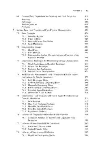
![CLASSIFICATION ACCORDING TO CONSTRUCTION FEATURES 15
FIGURE 1.6 Standard shell types and front- and rear-end head types (From TEMA, 1999).
vacuum to ultrahigh pressure [over 100 MPa (15,000 psig)], from cryogenics to high
temperatures [about 11008C (20008F)] and any temperature and pressure differences
between the fluids, limited only by the materials of construction. They can be designed
for special operating conditions: vibration, heavy fouling, highly viscous fluids, erosion,
corrosion, toxicity, radioactivity, multicomponent mixtures, and so on. They are the
most versatile exchangers, made from a variety of metal and nonmetal materials (such
as graphite, glass, and Teflon) and range in size from small [0.1m2 (1 ft2)] to supergiant
[over 105m2 (106 ft2)] surface area. They are used extensively as process heat exchangers](https://image.slidesharecdn.com/fundamentalsofheatexchangerdesign-131001160835-phpapp01-141008073824-conversion-gate02/85/Fundamentalsofheatexchangerdesign-131001160835-phpapp01-60-320.jpg)


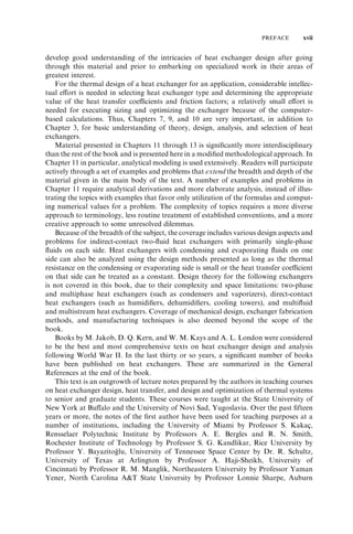
![CLASSIFICATION ACCORDING TO CONSTRUCTION FEATURES 25
Sealing between the two fluids is accomplished by elastomeric molded gaskets
[typically, 5 mm (0.2 in.) thick] that are fitted in peripheral grooves mentioned earlier
(dark lines in Fig. 1.17). Gaskets are designed such that they compress about 25% of
thickness in a bolted plate exchanger to provide a leaktight joint without distorting the
thin plates. In the past, the gaskets were cemented in the grooves, but now, snap-on
gaskets, which do not require cementing, are common. Some manufacturers offer special
interlocking types to prevent gasket blowout at high pressure differences. Use of a double
seal around the port sections, shown in Fig. 1.17, prevents fluid intermixing in the rare
event of gasket failure. The interspace between the seals is also vented to the atmosphere
to facilitate visual indication of leakage (Fig. 1.17). Typical gasket materials and their
range of applications are listed in Table 1.2, with butyl and nitrile rubber being most
common. PTFE (polytetrafluoroethylene) is not used because of its viscoelastic proper-ties.
Each plate has four corner ports. In pairs, they provide access to the flow passages on
either side of the plate. When the plates are assembled, the corner ports line up to form
distribution headers for the two fluids. Inlet and outlet nozzles for the fluids, provided in
the end covers, line up with the ports in the plates (distribution headers) and are con-nected
to external piping carrying the two fluids. A fluid enters at a corner of one end of
the compressed stack of plates through the inlet nozzle. It passes through alternate
channels{ in either series or parallel passages. In one set of channels, the gasket does
not surround the inlet port between two plates (see, e.g., Fig. 1.17a for the fluid 1 inlet
port); fluid enters through that port, flows between plates, and exits through a port at the
other end. On the same side of the plates, the other two ports are blocked by a gasket with
a double seal, as shown in Fig. 1.17a, so that the other fluid (fluid 2 in Fig. 1.17a) cannot
enter the plate on that side.{ In a 1 pass–1 pass} two-fluid counterflow PHE, the next
channel has gaskets covering the ports just opposite the preceding plate (see, e.g., Fig.
1.17b, in which now, fluid 2 can flow and fluid 1 cannot flow). Incidentally, each plate has
gaskets on only one side, and they sit in grooves on the back side of the neighboring plate.
In Fig. 1.16, each fluid makes a single pass through the exchanger because of alternate
gasketed and ungasketed ports in each corner opening. The most conventional flow
arrangement is 1 pass–1 pass counterflow, with all inlet and outlet connections on the
fixed end cover. By blocking flow through some ports with proper gasketing, either one
or both fluids could have more than one pass. Also, more than one exchanger can be
accommodated in a single frame. In cases with more than two simple 1-pass–1-pass heat
exchangers, it is necessary to insert one or more intermediate headers or connector plates
in the plate pack at appropriate places (see, e.g., Fig. 1.19). In milk pasteurization
applications, there are as many as five exchangers or sections to heat, cool, and regen-erate
heat between raw milk and pasteurized milk.
Typical plate heat exchanger dimensions and performance parameters are given in
Table 1.3. Any metal that can be cold-worked is suitable for PHE applications. The most
{A channel is a flow passage bounded by two plates and is occupied by one of the fluids. In contrast, a plate
separates the two fluids and transfers heat from the hot fluid to the cold fluid.
{ Thus with the proper arrangement, gaskets also distribute the fluids between the channels in addition to provid-ing
sealing to prevent leakage.
} In a plate heat exchanger, a pass refers to a group of channels in which the flow is in the same direction for one full
length of the exchanger (from top to bottom of the pack; see Fig. 1.65). In anm pass – n pass two-fluid plate heat
exchanger, fluid 1 flows through m passes and fluid 2 through n passes.](https://image.slidesharecdn.com/fundamentalsofheatexchangerdesign-131001160835-phpapp01-141008073824-conversion-gate02/85/Fundamentalsofheatexchangerdesign-131001160835-phpapp01-70-320.jpg)


![CLASSIFICATION ACCORDING TO CONSTRUCTION FEATURES 29
rates and depending on the allowed pressure drops of the two fluids, an arrangement of a
different number of passes for the two fluids may make a PHE advantageous. However,
care must be exercised to take full advantage of available pressure drop while multi-passing
one or both fluids.
Because of the long gasket periphery, PHEs are not suited for high-vacuum applica-tions.
PHEs are not suitable for erosive duties or for fluids containing fibrous materials.
In certain cases, suspensions can be handled; but to avoid clogging, the largest suspended
particle should be at most one-third the size of the average channel gap. Viscous fluids
can be handled, but extremely viscous fluids lead to flow maldistribution problems,
especially on cooling. Plate exchangers should not be used for toxic fluids, due to poten-tial
gasket leakage. Some of the largest units have a total surface area of about 2500m2
(27,000 ft2) per frame. Some of the limitations of gasketed PHEs have been addressed by
the new designs of PHEs described in the next subsection.
Major Applications. Plate heat exchangers were introduced in 1923 for milk pasteur-ization
applications and now find major applications in liquid–liquid (viscosities up to
10 Pa s) heat transfer duties. They are most common in the dairy, juice, beverage,
alcoholic drink, general food processing, and pharmaceutical industries, where their
ease of cleaning and the thermal control required for sterilization/pasteurization make
them ideal. They are also used in the synthetic rubber industry, paper mills, and in the
process heaters, coolers, and closed-circuit cooling systems of large petrochemical and
power plants. Here heat rejection to seawater or brackish water is common in many
applications, and titanium plates are then used.
Plate heat exchangers are not well suited for lower-density gas-to-gas applications.
They are used for condensation or evaporation of non-low-vapor densities. Lower vapor
densities limit evaporation to lower outlet vapor fractions. Specially designed plates are
now available for condensing as well as evaporation of high-density vapors such as
ammonia, propylene, and other common refrigerants, as well as for combined evapora-tion/
condensation duties, also at fairly low vapor densities.
1.5.2.2 Welded and Other Plate Heat Exchangers. One of the limitations of the
gasketed plate heat exchanger is the presence of gaskets, which restricts their use to
compatible fluids (noncorrosive fluids) and which limits operating temperatures and
pressures. To overcome this limitation, a number of welded plate heat exchanger designs
have surfaced with welded pairs of plates on one or both fluid sides. To reduce the
effective welding cost, the plate size for this exchanger is usually larger than that of the
gasketed PHE. The disadvantage of such a design is the loss of disassembling flexibility
on the fluid sides where the welding is done. Essentially, laser welding is done around
the complete circumference, where the gasket is normally placed. Welding on both sides
then results in higher limits on operating temperatures and pressures [3508C (6608F) and
4.0MPa (580 psig)] and allows the use of corrosive fluids compatible with the plate
material. Welded PHEs can accommodate multiple passes and more than two fluid
streams. A Platular heat exchanger can accommodate four fluid streams. Figure 1.20
shows a pack of plates for a conventional plate-and-frame exchanger, but welded on one
{ Special plate designs have been developed for phase-change applications.](https://image.slidesharecdn.com/fundamentalsofheatexchangerdesign-131001160835-phpapp01-141008073824-conversion-gate02/85/Fundamentalsofheatexchangerdesign-131001160835-phpapp01-74-320.jpg)
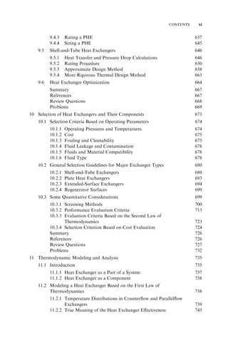
![30 CLASSIFICATION OF HEAT EXCHANGERS
FIGURE 1.20 Section of a welded plate heat exchanger. (Courtesy of Alfa Laval Thermal, Inc.,
Richmond, VA.)
fluid side. Materials used for welded PHEs are stainless steel, Hastelloy, nickel-based
alloys, and copper and titanium.
A Bavex welded-plate heat exchanger with welded headers is shown in Fig. 1.21. A
Stacked Plate Heat Exchanger is another welded plate heat exchanger design (from
Packinox), in which rectangular plates are stacked and welded at the edges. The physical
size limitations of PHEs [1.2m wide 4m long maximum (4 13 ft)] are considerably
extended to 1.5m wide20m long (566 ft) in Packinox exchangers. A maximum
surface area of over 10,000m2 (100,000 ft2) can be accommodated in one unit. The
potential maximum operating temperature is 8158C (15008F) with an operating pressure
of up to 20 MPa (3000 psig) when the stacked plate assembly is placed in a cylindrical
pressure vessel. For inlet pressures below 2 MPa (300 psig) and inlet temperatures below
2008C (4008F), the plate bundle is not placed in a pressure vessel but is bolted between
two heavy plates. Some applications of this exchanger are for catalytic reforming, hydro-sulfurization,
and crude distillation, and in a synthesis converter feed effluent exchanger
for methanol and for a propane condenser.
A vacuum brazed plate heat exchanger is a compact PHE for high-temperature and
high-pressure duties, and it does not have gaskets, tightening bolts, frame, or carrying
and guide bars. It consists simply of stainless steel plates and two end plates, all generally
copper brazed, but nickel brazed for ammonia units. The plate size is generally limited to
0.3m2. Such a unit can be mounted directly on piping without brackets and foundations.
Since this exchanger cannot be opened, applications are limited to negligible fouling
cases. The applications include water-cooled evaporators and condensers in the refrig-eration
industry, and process water heating and heat recovery.
A number of other plate heat exchanger constructions have been developed to address
some of the limitations of the conventional PHEs. A double-wall PHE is used to avoid
mixing of the two fluids. A wide-gap PHE is used for fluids having a high fiber content or
coarse particles/slurries. A graphite PHE is used for highly corrosive fluids. A flow-flex
exchanger has plain fins on one side between plates and the other side has conventional
plate channels, and is used to handle asymmetric duties (a flow rate ratio of 2 : 1 and
higher). A PHE evaporator has an asymmetric plate design to handle mixed process flows
(liquid and vapors) and different flow ratios.](https://image.slidesharecdn.com/fundamentalsofheatexchangerdesign-131001160835-phpapp01-141008073824-conversion-gate02/85/Fundamentalsofheatexchangerdesign-131001160835-phpapp01-75-320.jpg)


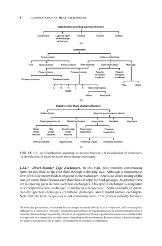
![40 CLASSIFICATION OF HEAT EXCHANGERS
Fig. 7.29c. Strip fins are also referred to as offset fins, lance-offset fins, serrated fins, and
segmented fins. Many variations of interrupted fins are used in industry since they employ
the materials of construction more efficiently than do plain fins and are therefore used
when allowed by the design constraints.
Plate-fin exchangers are generally designed for moderate operating pressures [less
than about 700 kPa gauge (100 psig)], although plate-fin exchangers are available
commercially for operating pressures up to about 8300 kPa gauge (1200 psig).
Recently, a condenser for an automotive air-conditioning system (see Fig. 1.27) using
carbon dioxide as the working fluid has been developed for operating pressures of 14
MPa (2100 psia). A recently developed titanium plate-fin exchanger (manufactured by
superelastic deformation and diffusion bonding, shown in Fig. 1.30) can take 35 MPa
(5000 psig) and higher pressures. The temperature limitation for plate-fin exchangers
depends on the method of bonding and the materials employed. Such exchangers have
been made from metals for temperatures up to about 8408C (15508F) and made from
ceramic materials for temperatures up to about 11508C (21008F) with a peak temperature
of 13708C (25008F). For ventilation applications (i.e., preheating or precooling of incom-ing
air to a building/room), the plate-fin exchanger is made using Japanese treated
(hygroscopic) paper and has the operating temperature limit of 508C (1228F). Thus,
FIGURE 1.30 Process of manufacturing of a super elastically deformed diffusion bonded plate-fin
exchanger (From Reay, 1999).](https://image.slidesharecdn.com/fundamentalsofheatexchangerdesign-131001160835-phpapp01-141008073824-conversion-gate02/85/Fundamentalsofheatexchangerdesign-131001160835-phpapp01-85-320.jpg)


![46 CLASSIFICATION OF HEAT EXCHANGERS
and sealed permanently at both ends. The inner surfaces of a heat pipe are usually lined
with a capillary wick (a porous lining, screen, or internally grooved wall). The wick is
what makes the heat pipe unique; it forces condensate to return to the evaporator by the
action of capillary force. In a properly designed heat pipe, the wick is saturated with the
liquid phase of the working fluid, while the remainder of the tube contains the vapor
phase. When heat is applied at the evaporator by an external source, the working fluid in
the wick in that section vaporizes, the pressure increases, and vapor flows to the con-denser
section through the central portion of the tube. The vapor condenses in the
condenser section of the pipe, releasing the energy of phase change to a heat sink (to a
cold fluid, flowing outside the heat pipe; see Fig. 1.37). The heat applied at the evaporator
section tries to dry the wick surface through evaporation, but as the fluid evaporates, the
liquid–vapor interface recedes into the wick surface, causing a capillary pressure to be
developed. This pressure is responsible for transporting the condensed liquid back to
the evaporator section, thereby completing a cycle. Thus, a properly designed heat pipe
can transport the energy of phase change continuously from the evaporator to the con-denser
without drying out the wick. The condensed liquid may also be pumped back to
the evaporator section by the capillary force or by the force of gravity if the heat pipe is
inclined and the condensation section is above the evaporator section. If the gravity force
is sufficient, no wick may be necessary. As long as there is a temperature difference
between the hot and cold gases in a heat pipe heat exchanger, the closed-loop evapora-tion–
condensation cycle will be continuous, and the heat pipe will continue functioning.
Generally, there is a small temperature difference between the evaporator and condenser
section [about 58C (98F) or so], and hence the overall thermal resistance of a heat pipe in
a heat pipe exchanger is small. Although water is a common heat pipe fluid, other fluids
are also used, depending on the operating temperature range.
A heat pipe heat exchanger (HPHE), shown in Fig. 1.36 for a gas-to-gas application,
consists of a number of finned heat pipes (similar to an air-cooled condenser coil)
mounted in a frame and used in a duct assembly. Fins on the heat pipe increase the
surface area to compensate for low heat transfer coefficients with gas flows. The fins can
be spirally wrapped around each pipe, or a number of pipes can be expanded into flat
plain or augmented fins. The fin density can be varied from side to side, or the pipe may
contain no fins at all (liquid applications). The tube bundle may be horizontal or vertical
with the evaporator sections below the condenser sections. The tube rows are normally
staggered with the number of tube rows typically between 4 and 10. In a gas-to-gas
HPHE, the evaporator section of the heat pipe spans the duct carrying the hot exhaust
gas, and the condenser section is located in the duct through which the air to be preheated
flows. The HPHE has a splitter plate that is used primarily to prevent mixing between the
two gas streams, effectively sealing them from one another. Since the splitter plate is thin,
a heat pipe in a HPHE does not have the usual adiabatic section that most heat pipes
have.
Unit size varies with airflow. Small units have a face size of 0.6m (length) by 0.3m
(height), and the largest units may have a face size up to 5m 3 m. In the case of gas-to-liquid
heat exchangers, the gas section remains the same, but because of the higher
external heat transfer coefficient on the liquid side, it need not be finned externally or
can even be shorter in length.
The heat pipe performance is influenced by the angle of orientation, since gravity
plays an important role in aiding or resisting the capillary flow of the condensate.
Because of this sensitivity, tilting the exchanger may control the pumping power and
ultimately the heat transfer. This feature can be used to regulate the performance of a](https://image.slidesharecdn.com/fundamentalsofheatexchangerdesign-131001160835-phpapp01-141008073824-conversion-gate02/85/Fundamentalsofheatexchangerdesign-131001160835-phpapp01-91-320.jpg)


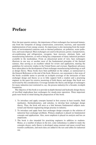
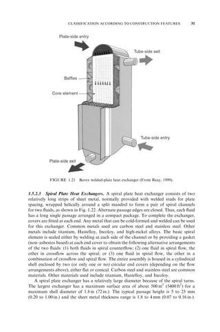
![52 CLASSIFICATION OF HEAT EXCHANGERS
FIGURE 1.43 Continuous-passage matrices for a rotary regenerator: (a) notched plate;
(b) triangular passage.
to minimize the primary leakage from the high-pressure fluid to the low-pressure
fluid.
A number of seal configurations are used in rotary regenerators. Two common shapes
are shown in Fig. 1.44. For the annular sector–shaped seals shown in Fig. 1.44a, flow
passages at every radial location experience the same flow exposure and seal-coverage
histories. For the uniform-width seals in Fig. 1.44b, flow passages at different radial
locations experience different flow exposure and seal coverage. For regenerators with
seals of equal area but arbitrary shape, the regenerator effectiveness is highest for annular
sector–shaped seals (Beck and Wilson, 1996).
Rotary regenerators have been designed for surface area densities of up to about
6600m2/m3 (2000 ft2/ft3). They can employ thinner stock material, resulting in the lowest
amount of material for a given effectiveness and pressure drop of any heat exchanger
known today. Metal rotary regenerators have been designed for continuous operating
inlet temperatures up to about 7908C (14508F). For higher-temperature applications,
ceramic matrices are used. Plastics, paper, and wool are used for regenerators operating
below 658C (1508F). Metal and ceramic regenerators cannot withstand large pressure
differences [greater than about 400 kPa (60 psi)] between hot and cold gases, because the
design of seals (wear and tear, thermal distortion, and subsequent leakage) is the single
most difficult problem to resolve. Plastic, paper, and wool regenerators operate approxi-
FIGURE 1.44 Seals used in rotary regenerators: (a) annular sector shaped; (b) uniform width
shape (Beck and Wilson, 1996).](https://image.slidesharecdn.com/fundamentalsofheatexchangerdesign-131001160835-phpapp01-141008073824-conversion-gate02/85/Fundamentalsofheatexchangerdesign-131001160835-phpapp01-97-320.jpg)
![CLASSIFICATION ACCORDING TO CONSTRUCTION FEATURES 53
mately at atmospheric pressure. Seal leakage can reduce the regenerator effectiveness
significantly. Rotary regenerators also require a power input to rotate the core from one
fluid to the other at the rotational speed desired.
Typical power plant regenerators have a rotor diameter up to 10m (33 ft) and
rotational speeds in the range 0.5 to 3 rpm (rev per min). Air-ventilating regenerators
have rotors with diameters of 0.25 to 3m (0.8 to 9.8 ft) and rotational speeds up to 10
rpm. Vehicular regenerators have diameters up to 0.6m (24 in.) and rotational speeds up
to 18 rpm.
Ljungstrom air preheaters for thermal power plants, commercial and residential oil-and
coal-fired furnaces, and regenerators for the vehicular gas turbine power plants are
typical examples of metal rotary regenerators for preheating inlet air. Rotary regenera-tors
are also used in chemical plants and in preheating combustion air in electricity
generation plants for waste heat utilization. Ceramic regenerators are used for high-temperature
incinerators and the vehicular gas turbine power plant. In air-conditioning
and industrial process heat recovery applications, heat wheels are made from knitted
aluminum or stainless steel wire matrix, wound polyester film, plastic films, and honey-combs.
Even paper, wettable nylon, and polypropylene are used in the enthalpy or
hygroscopic wheels used in heating and ventilating applications in which moisture is
transferred in addition to sensible heat.
1.5.4.2 Fixed-Matrix Regenerator. This type is also referred to as a periodic-flow,
fixed-bed, valved, or stationary regenerator. For continuous operation, this exchanger
has at least two identical matrices operated in parallel, but usually three or four, shown
in Figs. 1.45 and 1.46, to reduce the temperature variations in outlet-heated cold gas in
high-temperature applications. In contrast, in a rotary or rotating hood regenerator, a
single matrix is sufficient for continuous operation.
Fixed-matrix regenerators have two types of heat transfer elements: checkerwork and
pebble beds. Checkerwork or thin-plate cellular structure are of two major categories:
(1) noncompact regenerators used for high-temperature applications [925 to 16008C
(1700 to 29008F)] with corrosive gases, such as a Cowper stove (Fig. 1.41) for a blast
furnace used in steel industries, and air preheaters for coke manufacture and glass melt-ing
tanks made of refractory material; and (2) highly compact regenerators used for low-to
high-temperature applications, such as in cryogenic process for air separation, in
refrigeration, and in Stirling, Ericsson, Gifford, and Vuileumier cycle engines. The regen-erator,
a key thermodynamic element in the Stirling engine cycle, has only one matrix,
and hence it does not have continuous fluid flows as in other regenerators. For this
reason, we do not cover the design theory of a Stirling regenerator.
Cowper stoves are very large with an approximate height of 35m(115 ft) and diameter
of 7.5m (25 ft). They can handle large flow rates at inlet temperatures of up to 12008C
(22008F). A typical cycle time is between 1 and 3 h. In a Cowper stove, it is highly
desirable to have the temperature of the outlet heated (blast) air approximately constant
with time. The difference between the outlet temperatures of the blast air at the beginning
and end of a period is referred to as a temperature swing. To minimize the temperature
swing, three or four stove regenerators, shown in Figs. 1.45 and 1.46, are employed. In
the series parallel arrangement of Fig. 1.45, part of the cold air (blast) flow is bypassed
around the stove and mixed with the heated air (hot blast) leaving the stove. Since the
stove cools as the blast is blown through it, it is necessary constantly to decrease the
amount of the blast bypassed while increasing the blast through the stove by a corre-](https://image.slidesharecdn.com/fundamentalsofheatexchangerdesign-131001160835-phpapp01-141008073824-conversion-gate02/85/Fundamentalsofheatexchangerdesign-131001160835-phpapp01-98-320.jpg)


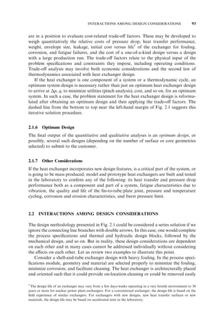


![HEAT EXCHANGER DESIGN METHODOLOGY 83
effectiveness, the heat load, fluid characteristics (such as fouling and corrosion ability),
cost, and others. For a relatively small heat load (i.e., smaller than 500 kW), a double-pipe
heat exchanger would be a cost-effective solution. Also, for higher performance, a
multitube double-pipe heat exchanger with or without fins should be considered if cost
considerations support this decision. See Example 2.4 for the inclusion of cost considera-tions
in a heat exchanger selection.
Finally, a decision should be made whether to use finned or plain tubes in the double-pipe
multitube heat exchanger selected. Due to the fact that the heat exchanger should
accommodate both a gas and a liquid, the heat transfer conductance (hA) on the gas side
(with low gas mass flow rate) will be low. Hence, employing fins on the gas side will yield
a more compact unit with approximately balanced hA values on the gas and liquid sides.
Note also that the tube fluid (liquid hydrocarbon) is more prone to fouling. So a double-pipe
multitube heat exchanger with finned tubes on the hydrocarbon gas side and liquid
hydrocarbon on the tube side has to be suggested as a feasible workable design.
2.1.2 Thermal and Hydraulic Design
Heat exchanger thermal/hydraulic design procedures (the second block from the top in
Fig. 2.1) involve exchanger rating (quantitative heat transfer and pressure drop evalua-tion)
and/or exchanger sizing. This block is the heart of this book, covered in Chapters 3
through 9. Only two important relationships constitute the entire thermal design
procedure. These are:
1. Enthalpy rate equations
q ¼ qj
¼ m_ j hj
ð2:1Þ
one for each of the two fluids (i.e., j ¼ 1, 2)
2. Heat transfer rate equation or simply the rate equation [see also the equality on the
left-hand side in Eq. (1.4)]
q ¼ UATm
ð2:2Þ
Equation (2.1) is a well-known relationship from thermodynamics. It relates the heat
transfer rate q with the enthalpy rate change for an open nonadiabatic system with a
single bulk flow stream (either j ¼ 1 or 2) entering and leaving the system under isobaric
conditions. For single-phase fluids in a heat exchanger, the enthalpy rate change is equal
to m_ j hj
¼ ðm_ cp
Þ
j Tj
¼ ðm_ cp
Þ
j Tj;i
Tj;o
. Equation (2.2) reflects a convection–
conduction heat transfer phenomenon in a two-fluid heat exchanger. The heat transfer
rate is proportional to the heat transfer area A and mean temperature difference Tm
between the fluids. This mean temperature difference is a log-mean temperature differ-ence
(for counterflow and parallelflow exchangers) or related to it in a way that involves
terminal temperature differences between the fluids such as (Th;i
Tc;o) and (Th;o
Tc;i).
It is discussed in Section 3.7.2. The coefficient of proportionality in Eq. (2.2) is the overall
heat transfer coefficient U (for the details, see Section 3.2.4). Solving a design problem
means either determining A (or UA) of a heat exchanger to satisfy the required terminal
values of some variables (the sizing problem), or determining the terminal values of the
variables knowing the heat exchanger physical size A or overall conductance UA (the](https://image.slidesharecdn.com/fundamentalsofheatexchangerdesign-131001160835-phpapp01-141008073824-conversion-gate02/85/Fundamentalsofheatexchangerdesign-131001160835-phpapp01-128-320.jpg)

![86 OVERVIEW OF HEAT EXCHANGER DESIGN METHODOLOGY
hydraulic design procedures, including optimization (the second major dashed-line
block in Fig. 2.1), are summarized in Chapter 9.
Example 2.2 Consider a heat exchanger as a black box with two streams entering
and subsequently leaving the exchanger without being mixed. Assume the validity of
both Eqs. (2.1) and (2.2). Also take into account that m_ j hj
¼ ðm_ cp
Þ
jTj , where
Tj
¼ Tj;i
Tj;o
. Note that regardless of the actual definition used, Tm must be a
function of terminal temperatures (Th;i ;Th;o;Tc;i ;Tc;o). With these quite general assump-tions,
answer the following two simple questions:
(a) How many variables of the seven used on the right-hand sides of Eqs. (2.1) and
(2.2) should minimally be known, and how many can stay initially unknown, to
be able to determine all design variables involved?
(b) Using the conclusion from question (a), determine how many different problems
of sizing a heat exchanger (UA must be unknown) can be defined if the set of
variables includes only the variables on the right-hand sides of Eqs. (2.1) and (2.2)
[i.e., ðm_ cp
Þ
j , Tj;i , Tj;o with j ¼ 1 or 2, and UA].
SOLUTION
Problem Data: A heat exchanger is considered as a black box that changes the set of inlet
temperatures Tj;i of the two fluids [with ðm_ cp
Þ
j , j ¼ 1, 2] into the set of their respective
outlet temperatures Tj;o
ð j ¼ 1; 2Þ through heat transfer characterized by Eq. (2.2) (i.e.,
by the magnitude of UA). So in this problem, we have to deal with the following
variables: ðm_ cp
Þ
1, ðm_ cp
Þ
2, T1;i , T1;o, T2;i , T2;o, and UA.
Determine: How many of the seven variables listed must be known to be able to deter-mine
all the variables involved in Eqs. (2.1) and (2.2)? Note that Eq. (2.1) represents two
relationships, one for each of the two fluids. How many different sizing problems (with at
least UA unknown) can be defined?
Assumptions: The heat exchanger is adiabatic; the enthalpy changes in enthalpy rate
equations, Eq. (2.1), can be determined by m_ j hj
¼ ðm_ cp
Þ
j Tj ; and the heat transfer
rate can be determined by Eq. (2.2).
Analysis: (a) The answer to the first question is trivial and can be devised by straight-forward
inspection of the three equations given by Eqs. (2.1) and (2.2). Note that the left-hand
sides of these equalities are equal to the same heat transfer rate. This means that
these three equations can be reduced to two equalities by eliminating heat transfer rate q.
For example,
ðm_ cp
Þ
1 T1;i
T1;o
¼ UATm
ðm_ cp
Þ
2 T2;i
T2;o
¼ UATm
So we have two relationships between seven variables [note that
Tm
¼ f ðT1;i ; T1;o; T2;i ; T2;o
Þ]. Using the two equations, only two unknowns can be
determined. Consequently, the remaining five must be known.
(b) The answer to the second question can now be obtained by taking into account the
fact that (1) UA must be treated as an unknown in all the cases considered (a sizing](https://image.slidesharecdn.com/fundamentalsofheatexchangerdesign-131001160835-phpapp01-141008073824-conversion-gate02/85/Fundamentalsofheatexchangerdesign-131001160835-phpapp01-131-320.jpg)
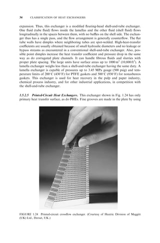
![HEAT EXCHANGER DESIGN METHODOLOGY 87
TABLE E2.2 Heat Exchanger Sizing Problem Types
Problem UA ðm_ cp
Þ
1
ðm_ cp
Þ
2 T1;i T1;o T2;i T2;o
1
2
3
4
5
6
, Unknown variable; , known variable.
problem), and (2) only two variables can be considered as unknown since we have only
two equations [Eqs. (2.1) and (2.2)] at our disposal. Thus, the number of combinations
among the seven variables is six (i.e., in each case the two variables will be unknown and
the remaining five must be known). This constitutes the list of six types of different sizing
problems given in Table E2.2.
Discussion and Comments: Among the six types of sizing problems, four have both heat
capacity rates [i.e., the products ðm_ cp
Þ
j known]; and in addition to UA, the unknown is
one of the four terminal temperatures. The remaining two problem types presented in
Table E2.2 have one of the two heat capacity rates unknown and the other heat capacity
rate and all four temperatures known.
Exactly the same reasoning can be applied to devise a total of 15 rating problems
(in each of these problems, the product UA must stay known). A complete set of design
problems (including both the sizing and rating problems), devised in this manner, is
given in Table 3.11.
2.1.3 Mechanical Design
Mechanical design is essential to ensure the mechanical integrity of the exchanger under
steady-state, transient, startup, shutdown, upset, and part-load operating conditions
during its design life. As mentioned in the beginning of Chapter 1, the exchanger consists
of heat exchanging elements (core or matrix where heat transfer takes place) and fluid
distribution elements (such as headers, manifolds, tanks, inlet/outlet nozzles, pipes, and
seals, where ideally, no heat transfer takes place). Mechanical/structural design should be
performed individually for these exchanger elements. Also, one needs to consider the
structural design of heat exchanger mounting. Refer to the third dashed-line block from
the top in Fig. 2.1 for a discussion of this section.
The heat exchanger core is designed for the desired structural strength based on the
operating pressures, temperatures, and corrosiveness or chemical reaction of fluids with
materials. Pressure/thermal stress calculations are performed to determine the thick-nesses
of critical parts in the exchangers, such as the fin, plate, tube, shell, and tubesheet.
A proper selection of the material and the method of bonding (such as brazing, soldering,
welding, or tension winding) fins to plates or tubes is made depending on the operating
temperatures, pressures, types of fluids used, fouling and corrosion potential, design life,
and so on. Similarly, proper bonding techniques should be developed and used for tube-](https://image.slidesharecdn.com/fundamentalsofheatexchangerdesign-131001160835-phpapp01-141008073824-conversion-gate02/85/Fundamentalsofheatexchangerdesign-131001160835-phpapp01-132-320.jpg)


![HEAT EXCHANGER DESIGN METHODOLOGY 91
tenance, repair, cleaning, lost production/downtime due to failure, energy cost asso-ciated
with the utility (steam, fuel, water) in conjunction with the exchanger in the
network, and decommissioning costs. Some of the cost estimates are difficult to obtain
and best estimates are made at the design stage.
Example 2.4 A heat exchanger designer needs to make a preliminary selection of a heat
exchanger type for known heat transfer performance represented by q=Tm [Eqs. (1.4)
and Eq. (2.2)]. The exchanger should operate with q=Tm
¼ 6:3 104 W/K. The criter-ion
for selection at that point in the design procedure is the magnitude of the unit cost per
unit of q=Tm. From a preliminary analysis, the engineer has already selected four
possible workable design types as follows: (1) a shell-and-tube heat exchanger, (2) a
double-pipe heat exchanger, (3) a plate-and-frame heat exchanger, and (4) a welded
plate heat exchanger. From the empirical data available, the unit costs (in dollars per
unit of q=Tm) for the two values of q=Tm are given in Table E2.4A. Idealize the
dependence of the unit cost vs. q=Tm as logarithmic. What is going to be the engineer’s
decision? Discuss how this decision changes with a change in the heat exchanger perfor-mance
level.
SOLUTION
Problem Data and Schematic: From the available empirical data, the heat exchanger unit
cost per unit of heat exchanger performance level is known (see Table E2.4A).
Schematics of heat exchanger types selected are given in Figs. 1.5, 1.15, 1.16, and 1.20.
Determine: The heat exchanger type for a given performance. Formulate the decision
using the unit cost per unit of q=Tm as a criterion.
Assumptions: The cost of heat exchangers vs. q=Tm (W/K) is a logarithmic relationship.
All heat exchanger types selected represent workable designs (meet process/design
specifications). The heat exchanger performance is defined by q=Tm as given by Eq.
(1.4).
Analysis: The analysis should be based on data provided in Table E2.4A. Because there
are no available data for the performance level required, an interpolation should be
performed. This interpolation must be logarithmic. In Table E2.4B, the interpolated
data are provided along with the data from Table E2.4A.
TABLE E2.4A Unit Cost for q=Tm
Heat Exchanger Type
$/(W/K) for q=Tm
5 103 W/K 1 105 W/K
Shell-and-tube 0.91 0.134
Double pipe 0.72 0.140
Plate-and-frame 0.14 0.045
Welded plate 1.0 0.108
Source: Modified from Hewitt and Pugh (1998).](https://image.slidesharecdn.com/fundamentalsofheatexchangerdesign-131001160835-phpapp01-141008073824-conversion-gate02/85/Fundamentalsofheatexchangerdesign-131001160835-phpapp01-136-320.jpg)


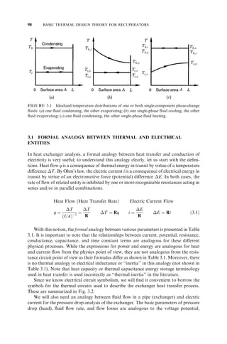
![FORMAL ANALOGY BETWEEN THERMAL AND ELECTRICAL ENTITIES 99
TABLE 3.1 Analogies and Nonalogies between Thermal and Electrical Parameters
Parameter Electrical Thermal
Current i ampere, A q W, Btu/hr
Potential E volts, V T 8CðKÞ; 8Fð8RÞ
Resistance R ohms, ; V/A R ¼ 1=UA 8C=W; 8F-hr/Btu
Conductance G siemens, S, A/V UA W/8C, Btu/hr-8F
Capacitance C farads, F, A s/V C W s=8C; Btu/8F
Time constant RC s R C s, hr
Power iE W q W, Btu/hr
Energy
ð
0
iE d J, W s
current, and resistance.
Analogies
Nonanalogies
y
Since the flow losses are measured in terms of the pressure loss
or head or fluid column, which have the same units as the potential, this analogy is not as
well defined as the analogy between heat transfer and electric current. Again, the rela-tionship
between analogous parameters for fluid flow is not linear for transition and
turbulent flows or developing laminar flows in pipes.
ð
0
q d J, Btu
FIGURE 3.2 Thermal circuit symbolism.
y
Pipe and duct design based on one-dimensional lumped parameter analysis typically defines the flow resistance or
the flow loss coefficient K as equal to the number of velocity heads lost due to frictional effects [see Eq. (6. 53)].](https://image.slidesharecdn.com/fundamentalsofheatexchangerdesign-131001160835-phpapp01-141008073824-conversion-gate02/85/Fundamentalsofheatexchangerdesign-131001160835-phpapp01-144-320.jpg)
![100 BASIC THERMAL DESIGN THEORY FOR RECUPERATORS
3.2 HEAT EXCHANGER VARIABLES AND THERMAL CIRCUIT
In this section, starting with the assumptions built into heat exchanger design theory, the
basic problem for the exchanger heat transfer analysis is formulated. This includes the
differential equations used for the analysis as well as a list of independent and dependent
variables associated with heat exchanger design and analysis problems. Next, the basic
definitions of important dimensional variables and important terminologies are intro-duced.
Finally, the thermal circuit, and expressions for UA and wall temperatures are
presented.
3.2.1 Assumptions for Heat Transfer Analysis
To analyze the exchanger heat transfer problem, a set of assumptions are introduced so
that the resulting theoretical models are simple enough for the analysis. The following
assumptions and/or idealizations are made for the exchanger heat transfer problem
formulations: the energy balances, rate equations, boundary conditions, and subsequent
y
analysis [see, e.g., Eqs. (3.2) and (3.4) through (3.6) in differential or integral form].
1. The heat exchanger operates under steady-state conditions [i.e., constant flow
rates and fluid temperatures (at the inlet and within the exchanger) independent
of time].
2. Heat losses to or from the surroundings are negligible (i.e. the heat exchanger
outside walls are adiabatic).
3. There are no thermal energy sources or sinks in the exchanger walls or fluids, such
as electric heating, chemical reaction, or nuclear processes.
4. The temperature of each fluid is uniform over every cross section in counterflow
and parallelflow exchangers (i.e., perfect transverse mixing and no temperature
gradient normal to the flow direction). Each fluid is considered mixed or unmixed
from the temperature distribution viewpoint at every cross section in single-pass
crossflow exchangers, depending on the specifications. For a multipass exchan-ger,
the foregoing statements apply to each pass depending on the basic flow
arrangement of the passes; the fluid is considered mixed or unmixed between
passes as specified.
5. Wall thermal resistance is distributed uniformly in the entire exchanger.
6. Either there are no phase changes (condensation or vaporization) in the fluid
streams flowing through the exchanger or the phase change occurs under the
following condition. The phase change occurs at a constant temperature as for
a single-component fluid at constant pressure; the effective specific heat cp;eff for
the phase-changing fluid is infinity in this case, and hence Cmax
¼ m_ cp;eff
!1;
where m_ is the fluid mass flow rate.
7. Longitudinal heat conduction in the fluids and in the wall is negligible.
8. The individual and overall heat transfer coefficients are constant (independent of
temperature, time, and position) throughout the exchanger, including the case of
phase-changing fluids in assumption 6.
y
The complete set of differential equations and boundary conditions describing the mathematical models of heat
exchangers, based on these assumptions, is presented in Section 11.2.](https://image.slidesharecdn.com/fundamentalsofheatexchangerdesign-131001160835-phpapp01-141008073824-conversion-gate02/85/Fundamentalsofheatexchangerdesign-131001160835-phpapp01-145-320.jpg)


![HEAT EXCHANGER VARIABLES AND THERMAL CIRCUIT 103
The negative signs in this equation are a result of Th and Tc decreasing with increasing
A (these temperatures decrease with increasing flow length x as shown in Fig. 1.50);
y
also,
dq is the heat transfer rate from the hot to cold fluid, C ¼ m_ cp is the heat capacity rate of
the fluid, m_ is the fluid flow rate, cp is the fluid specific heat at constant pressure, T is the
fluid temperature, and the subscripts h and c denote hot and cold fluids, respectively. The
heat capacity rate C J/s 8C (Btu/hr 8F) is the amount of heat in joules (Btu) that must
be added to or extracted from the fluid stream per second (hour) to change its tempera-ture
by 18C ð8FÞ. The product m_ cp
¼ C appears in the energy balance [Eq. (3.2)] for
constant cp, and hence C is commonly used in the heat exchanger analysis instead of m_
and cp as two parameters separately.
In general, for any isobaric change of state, Eq. (3.2) should be replaced by
dq ¼ m_ h dhh
¼ m_ c dhc
ð3:3Þ
where h is the fluid specific enthalpy, J/kg (Btu/lbm). If the change of state is a phase
change, enthalpy differences should be replaced by enthalpies of phase change (either
enthalpy of evaporation or enthalpy of condensation). However, cp can be assumed as
infinity for condensing or evaporating single-component fluid streams. Hence, the phase-changing
stream can be treated as a ‘‘single-phase’’ fluid having T ¼ q=C or
dT ¼ dq=C, with C being infinity for a finite q or dq since the T or dT ¼ 0 for
isothermal condensing or evaporating fluid streams (see Fig. 3.1). Note that here
T ¼ Th; i
Th;o or Tc;o
Tc;i as appropriate.
The overall heat transfer rate equation on a differential base for the surface area dA of
Fig. 3.3 is
dq ¼ UðTh
Tc
Þ
local dA ¼ U T dA ð3:4Þ
z
Thus for
where U is the local overall heat transfer coefficient to be defined in Eq. (3.20).
this differential element dA, the driving potential for heat transfer is the local temperature
difference ðTh
Tc
Þ ¼ T and the thermal conductance is UdA.
Integration of Eqs. (3.2) and (3.4) together over the entire heat exchanger surface for
specified inlet temperatures will result in an expression that will relate all important
operating variables and geometry parameters of the exchanger. The derivation of such
an expression for a counterflow exchanger will be presented in Section 3.3 together with
final results for many industrially important exchanger flow arrangements. The common
assumptions invoked for the derivation and integration of Eqs. (3.2) and (3.4) are
summarized in Section 3.2.1.
Two basic equations, energy conservation (balance) and rate equations, could also be
written on an overall basis for the entire exchanger as follows (under the conditions
implied by the above-mentioned idealizations):
y
The sign convention adopted in Eq. (3.2) leads to positive value of heat transfer rate change along each dx
element, and should be considered only as formal (i.e., not necessarily in agreement with thermodynamic con-vention
for heat).
z
Note that although the overall heat transfer coefficient U is idealized as constant (see assumption 8 in Section
3.2.1), it can vary significantly in a heat exchanger. In that case, the mean overall heat transfer coefficient Um is
obtained from local U data (see Section 4.2.3). Even though U ¼ Um
¼ constant throughout this chapter, we
distinguish between U and Um in Sections 3.2.3 and 3.2.4 to emphasize how the theory is developed using U and
Um.](https://image.slidesharecdn.com/fundamentalsofheatexchangerdesign-131001160835-phpapp01-141008073824-conversion-gate02/85/Fundamentalsofheatexchangerdesign-131001160835-phpapp01-148-320.jpg)


![HEAT EXCHANGER VARIABLES AND THERMAL CIRCUIT 107
NTUs (see Section 3.3.3 for the definition of NTU). The magnitude of the external
temperature cross is Tc; o
Th;o. Internal temperature cross refers to the case when locally
somewhere within the exchanger Tc becomes equal to Th (within a pass or in a segment of
the exchanger), and beyond that point along the flow length, Tc Th in that pass or
segment; subsequently, reverse heat transfer takes place (original cold fluid transferring
heat to the original hot fluid). The external temperature cross can occur with or without
the internal temperature cross; similarly an internal temperature cross can occur with or
without an external temperature cross (see Section 11.4.1).
3.2.4 Thermal Circuit and UA
To understand the exchanger overall heat transfer rate equation [Eq. (3.12)], consider the
thermal circuit model of Fig. 3.4. Scale or fouling deposit layers are also shown on each
side of the wall.
In the steady state, heat is transferred from the hot fluid to the cold fluid by the
following processes: convection to the hot fluid wall, conduction through the wall, and
subsequent convection from the wall to the cold fluid. In many heat exchangers, a fouling
film is formed as a result of accumulation of scale or rust formation, deposits from
the fluid, chemical reaction products between the fluid and the wall material, and/or
biological growth. This undesired fouling film usually has a low thermal conductivity
and can increase the thermal resistance to heat flow from the hot fluid to the cold fluid.
This added thermal resistance on individual fluid sides for heat conduction through the
fouling film is taken into account by a fouling factor
y
rf
¼ 1=hf , where the subscript f
denotes fouling (or scale); it is shown in Fig. 3.4. Thus, the heat transfer rate per unit
area at any section dx (having surface areas dAh, dAc, etc.) can be presented by the
appropriate convection and conduction rate equations as follows:
dq ¼
Th
Th; f
dRh
¼
Tw;h
dRh; f
Th; f
Tw;c
dRw
¼ Tw;h
¼
Tc; f
dRc; f
Tw;c
¼
Tc
dRc
Tc; f
ð3:15Þ
Alternatively
Tc
dRo
dq ¼ Th
¼ U dAðTh
Tc
Þ ð3:16Þ
where the overall differential thermal resistance dRo consists of component resistances in
series (similar to those shown in Fig. 3.4b for a heat exchanger):
1
U dA
¼ dRo
¼ dRh
þ dRh; f
þ dRw
þ dRc; f
þ dRc
ð3:17Þ
or
1
U dA
¼ 1
ðoh dAÞ
h
þ 1
ðohf dAÞ
h
þ dRw
þ 1
ðohf dAÞ
c
þ 1
ðoh dAÞ
c
ð3:18Þ
^R
y
We also refer to the fouling factor as the unit fouling thermal resistance or concisely as fouling resistance
rf
¼ Rf
¼ 1=hf
¼ f =kf where f is the thickness of fouling layer and kf is the thermal conductivity of the fouling
material. Refer to Section 13.1 for more details on the fouling resistance concept.](https://image.slidesharecdn.com/fundamentalsofheatexchangerdesign-131001160835-phpapp01-141008073824-conversion-gate02/85/Fundamentalsofheatexchangerdesign-131001160835-phpapp01-152-320.jpg)
![Various symbols in this equation are defined after Eq. (3.24). If we idealize that the heat
transfer surface area is distributed uniformly on each fluid side (see assumption 11 in
Section 3.2.1), the ratio of differential area on each fluid side to the total area on the
respective side remains the same; that is,
dA
A
¼ dAh
Ah
¼ dAc
Ac
¼ dAw
Aw
ð3:19Þ
Replacing differential areas of Eq. (3.18) by using corresponding terms of Eq. (3.19),
we get
1
UA
¼ 1
ðohAÞ
h
þ 1
ðohfAÞ
h
þ Rw
þ 1
ðohfAÞ
c
þ 1
ðohAÞ
c
ð3:20Þ
It should be emphasized that U and all h’s in this equation are assumed to be local. Using
the overall rate equation [Eq. (3.6)], the total heat transfer rate will be
q ¼ UmATm
¼ UmAðTh;e
Tc;e
Þ ¼ 1
Ro
ðTh;e
Tc;e
Þ ð3:21Þ
108 BASIC THERMAL DESIGN THEORY FOR RECUPERATORS
FIGURE 3.4 (a) Thermal resistances; (b) thermal circuit for a heat exchanger (From Shah, 1983).](https://image.slidesharecdn.com/fundamentalsofheatexchangerdesign-131001160835-phpapp01-141008073824-conversion-gate02/85/Fundamentalsofheatexchangerdesign-131001160835-phpapp01-153-320.jpg)


![HEAT EXCHANGER VARIABLES AND THERMAL CIRCUIT 111
Thus in specifying UA as a product, we don’t need to specify A explicitly. However,
the option of Ah, Ac, or Aw must be specified in evaluating U from the product UA since
Uh
6¼ Uc if Ah
6¼ Ac. It should be mentioned that the value of Ro
¼ 1=UA will always be
larger than the largest thermal resistance component of Eq. (3.23). This means that UA
will always be smaller than the minimum thermal conductance component [a reciprocal
of any one term of the right-hand side of Eq. (3.24)]. UA is referred to as the overall
thermal conductance.
If the overall rate equation is based on a unit surface area
q
A
¼ q
00 ¼ U Tm
ð3:29Þ
the unit overall thermal resistance is ^R
Ro
¼ 1=U. In this case, individual components of
resistances are also on a unit area basis, all based on either Ah or Ac explicitly as follows:
1
Uh
¼ 1
ðohÞ
h
þ 1
ðohf
Þ
h
þ RwAh
þ Ah=Ac
ðohf
Þ
c
þ Ah=Ac
ðohÞ
c
¼ ^R
Rh
þ 1
o;h
^R
Rh; f
þ ^R
Rw
Ah
Aw
þ 1
o;c
^R
Rc; f
Ah
Ac
þ ^R
Rc
Ah
Ac
ð3:30aÞ
1
Uc
¼ Ac=Ah
ðohÞ
h
þ Ac=Ah
ðohf
Þ
h
þ RwAc
þ 1
ðohf
Þ
c
þ 1
ðohÞ
c
¼ ^R
Rh
Ac
Ah
þ 1
o;h
^R
Rh; f
Ac
Ah
þ ^R
Rw
Ac
Aw
þ 1
o;c
^R
Rc; f
þ ^R
Rc
ð3:30bÞ
where 1=Uh is the unit overall thermal resistance based on the hot-fluid-side surface area.
Similarly, 1=Uc is defined. Also ^R
Rj
¼ 1=ðohÞ
j , j ¼ h or c are unit thermal resistances for
hot or cold fluids, ^R
Rf
¼ 1=hf
¼ unit thermal fouling resistance, and ^R
Rw
¼ w=kw
¼ unit
wall thermal resistance. For a plain tubular exchanger, o
¼ 1; then from Eq. (3.30), Uo
based on the tube outside surface area is given as follows after inserting the value of Rw
from the first equation of Eq. (3.26):
1
Uo
¼ 1
ho
þ 1
ho; f
þ do lnðdo=di
Þ
2kw
þ do
hi; f di
þ do
hidi
ð3:31aÞ
1
Ui
¼ di
hodo
þ di
ho; f do
þ di lnðdo=di
Þ
2kw
þ 1
hi; f
þ 1
hi
ð3:31bÞ
Here the subscripts o and i denote the tube outside and inside, respectively; 1=Uo and
1=Ui are the unit overall thermal resistances based on the tube outside and inside surface
area, respectively.
Knowledge of wall temperature in a heat exchanger is essential to determine
the localized hot spots, freeze points, thermal stresses, local fouling characteristics, or
boiling/condensing coefficients. In this case, Tw;h and Tw;c can be computed from
Eq. (3.22) on a local basis as follows:
Th
Tw;h
Rh
þ Rh; f
¼ Tw;c
Tc
Rc
þ Rc; f
ð3:32Þ](https://image.slidesharecdn.com/fundamentalsofheatexchangerdesign-131001160835-phpapp01-141008073824-conversion-gate02/85/Fundamentalsofheatexchangerdesign-131001160835-phpapp01-156-320.jpg)

![HEAT EXCHANGER VARIABLES AND THERMAL CIRCUIT 113
Analysis: The required heat transfer rate may be obtained from the overall energy
balance for the cold fluid [Eq. (3.5)].
q ¼ Cc
ðTc;o
Tc;i
Þ ¼ ðm_ cp
Þ
c
ðTc;o
Tc;i
Þ
¼ 180 kg=h
3600 s=h
ð4:19 J=g KÞð1000 g=kgÞð90 15Þ8C ¼ 15,713W
Apply the same Eq. (3.5) on the hot fluid side to find the outlet temperature for flue gas:
Th;o
¼ Th;i
q
ðm_ cp
Þ
h
Since
m_ h
¼ 900 kg=h
3600 s=h
¼ 0:25 kg=s
cp;h
¼ ð1:05 J=g KÞ ð1000 g=kgÞ ¼ 1050 J=kg K
we get
Th;o
¼ 1508C 15,713W
0:25 kg=s 1050 J=kg 8C
¼ 90:18C Ans:
Since U is based on A ¼ Ah
¼ doLNt, Eq. (3.31) reduces to the following form after
substituting the hot-fluid-side fouling factor (1=hf ) as zero, and replacing the subscripts o
and i of U and h with h and c, respectively.
R ¼ 1
^R
Uh
¼ 1
hh
þ 1
hh; f
þ do lnðdo=di
Þ
2kw
þ do
hc; f di
þ do
hcdi
¼ 1
120W=m2 K
þ 0:032m½lnð32mm=25mmÞ
2 381W=m K
þ 0:002m2 K=W 0:032m
0:025m
þ 0:032m
120W=m2 K 0:025m
¼ ð0:00833 þ 0:00001 þ 0:00256 þ 0:00107Þm2 K=W ¼ 0:01197m2 K=W
ð69:6%Þ ð0:1%Þ ð21:4%Þ ð8:9%Þ
Hence,
Uh
¼ 83:54W=m2 K Ans:
Note that the controlling thermal resistance for this feedwater heater is 69.6% on the flue
gas side. Now the mean temperature difference can be determined from Eq. (3.12) as
Tm
¼ q
UhAh
¼ 15,713W
83:54W=m2 K 5m2
¼ 37:68C Ans:](https://image.slidesharecdn.com/fundamentalsofheatexchangerdesign-131001160835-phpapp01-141008073824-conversion-gate02/85/Fundamentalsofheatexchangerdesign-131001160835-phpapp01-158-320.jpg)


![seven-parameter problem
y
[Eq. (3.7)], to a three-parameter problem, [Eq. (3.50)] for a
given heat exchanger flow arrangement of two fluids.
Before discussing the physical significance of the two independent parameters C* and
NTU, let us introduce the definitions of the temperature effectiveness for the hot and cold
fluids. The temperature effectiveness h of the hot fluid is defined as a ratio of the
temperature drop of the hot fluid to the fluid inlet temperature difference:
h
¼ Th;i
Th;o
Th;i
Tc;i
¼ Th
Tmax
ð3:51Þ
Similarly, the temperature effectiveness of the cold fluid is defined as a ratio of the
temperature rise of the cold fluid to the fluid inlet temperature difference:
c
¼ Tc;o
Tc;i
Th;i
Tc;i
¼ Tc
Tmax
ð3:52Þ
From an energy balance [Eq. (3.5)], and definitions of h, and c, it can be shown that
Chh
¼ Ccc
ð3:53Þ
A comparison of temperature effectivenesses with Eq. (3.44) for the exchanger (heat
transfer) effectiveness reveals that they are related by
¼ Ch
Cmin
h
¼
h for Ch
¼ Cmin
h=C* for Ch
¼ Cmax
(
ð3:54Þ
¼ Cc
Cmax
c
¼
c for Cc
¼ Cmin
c=C* for Cc
¼ Cmax
(
ð3:55Þ
Now let us define and discuss C* and NTU.
3.3.2 Heat Capacity Rate Ratio C*
C* is simply a ratio of the smaller to larger heat capacity rate for the two fluid streams so
that C* 1. A heat exchanger is considered balanced when C* ¼ 1:
C* ¼ Cmin
Cmax
¼
ðm_ cp
Þ
min
ðm_ cp
Þ
max
¼
ðTc;o
Tc;i
Þ=ðTh;i
Th;o
Þ for Ch
¼ Cmin
ðTh;i
Th;o
Þ=ðTc;o
Tc;i
Þ for Cc
¼ Cmin
(
ð3:56Þ
C* is a heat exchanger operating parameter since it is dependent on mass flow rates
and/or temperatures of the fluids in the exchanger. The Cmax fluid experiences a
smaller temperature change than the temperature change for the Cmin fluid in the absence
of extraneous heat losses, as can be found from the energy balance:
q ¼ Ch Th
¼ Cc Tc
ð3:57Þ
118 BASIC THERMAL DESIGN THEORY FOR RECUPERATORS
y
In counting, we have considered only one dependent variable of Eq. (3.7).](https://image.slidesharecdn.com/fundamentalsofheatexchangerdesign-131001160835-phpapp01-141008073824-conversion-gate02/85/Fundamentalsofheatexchangerdesign-131001160835-phpapp01-163-320.jpg)


![Integrating this equation from the hot-fluid inlet (section I) to the outlet section (section
II) yields
Th;II
Tc;II
Th;I
Tc;I
¼ exp
UA
Ch
1 Ch
Cc
ð3:76Þ
It can be shown algebraically that the left-hand side of Eq. (3.76) is
Th;II
Tc;II
Th;I
Tc;I
¼ 1 ðTh;I
Th II
Þ=ðTh;I
Tc;II
Þ
1 ðTc;I
Tc II
Þ=ðTh;I
Tc;II
Þ
ð3:77Þ
Now employ the definitions of the temperature effectivenesses from Eqs. (3.51) and
(3.52), using the nomenclature of Fig. 3.6:
h
¼ Th;I
Th ;II
Th;I
Tc;II
c
¼ Tc;I
Tc;II
Th;I
Tc;II
ð3:78Þ
Substituting the definitions of h and c in Eq. (3.77), it reduces to
Th;II
Tc;II
Th;I
Tc;I
¼ 1 h
1 c
¼ 1 h
1 ðCh=Cc
Þh
ð3:79Þ
where Eq. (3.53) is used to obtain the last equality. Substituting Eq. (3.79) into (3.76) and
rearranging, we get
h
¼ 1 exp½ðUA=Ch
Þð1 Ch=Cc
Þ
1 ðCh=Cc
Þ exp½ðUA=Ch
Þð1 Ch=Cc
Þ
ð3:80Þ
Now the temperature effectiveness of the cold fluid, c, can be determined either
directly by employing its definition [Eq. (3.52)], or by substituting Eq. (3.80) into
(3.53). Using the second approach, gives us
c
¼ Ch
Cc
h
¼ 1 exp½ðUA=Cc
Þð1 Cc=Ch
Þ
ðCc=Ch
Þ exp½ðUA=Cc
Þð1 Cc=Ch
Þ
ð3:81Þ
Notice that the argument of the exponential terms has been rearranged. By multiplying
both numerator and denominator by exp fðUA=Cc
Þ½1 ðCc=Ch
Þg and rearranging, we
get
c
¼ 1 exp½ðUA=Cc
Þð1 Cc=Ch
Þ
1 ðCc=Ch
Þ exp½ðUA=Cc
Þð1 Cc=Ch
Þ
ð3:82Þ
A comparison of Eqs. (3.80) and (3.82) reveals that Eq. (3.82) can be obtained directly
from Eq. (3.80) by replacing the subscripts h with c and c with h.
To generalize the solution, let Cmin
¼ Cc, C* ¼ Cc=Ch and NTU ¼
UA=Cmin
¼ UA=Cc. In this case, ¼ c from Eq. (3.52), and Eq. (3.82) reduces to
¼ cf
¼ 1 exp½NTUð1 C*Þ
1 C* exp½NTUð1 C*Þ
ð3:83Þ
124 BASIC THERMAL DESIGN THEORY FOR RECUPERATORS](https://image.slidesharecdn.com/fundamentalsofheatexchangerdesign-131001160835-phpapp01-141008073824-conversion-gate02/85/Fundamentalsofheatexchangerdesign-131001160835-phpapp01-169-320.jpg)


![P-NTU RELATIONSHIPS 143
The P1-NTU1 relationship for the 1–n exchanger (one shell pass, even-n tube passes
with shell fluid mixed) is also presented in Table 3.6. Note that this 1–n exchanger ðn 4Þ
is stream asymmetric. The temperature effectiveness P1 of the 1–n exchanger ðn 2 and
even) is lower than that of the 1–2 exchanger for specified values of NTU1 and R1. The
maximum reduction in P1 of the 1–n exchanger over the 1–2 exchanger occurs at R1
¼ 1.
The thermal effectivenesses of the 1–n exchangers at R1
¼ 1 are shown in Table 3.7. From
a review of this table, if the P1-NTU1 expression of Table 3.6 for the 1–2 exchanger is
used for the 1–n exchanger ðn 4 and even), the error introduced is negligible for low
NTU1 (NTU1 3), particularly for R1
6¼ 1. However, if this error is not acceptable, it is
recommended to employ the P1-NTU1 expression [see Eq. (III.4) in Table 3.6] of the 1–4
exchanger for the 1–n exchanger for n 4 and even. When n!1, the 1–n exchanger
effectiveness approaches that of a crossflow exchanger with both fluids mixed, and the
formula is given in Table 3.6 as Eq. (III.5).
The P-NTU results are presented in Figs. 3.14, 3.15, and 3.16 for 1–2 TEMA G, H,
and J exchangers for comparisons with those in Fig. 3.13 for the 1–2 TEMA E exchanger.
3.6.1.2 Temperature Cross.
y
As defined earlier, the temperature cross refers to the
situation where the cold-fluid outlet temperature Tc;o is greater than the hot-fluid outlet
temperature Th;o; and in this case, the magnitude of the temperature cross is
ðTc; Þ. o
Th;o
It derives its name from fictitious (e.g., counterflow exchanger; see Fig.
1.50) or actual crossing (e.g., 1–2 TEMA E exchanger as shown in Fig. 3.17b) of the
temperature distributions of the hot and cold fluids in heat exchangers. Note that the
tube fluid temperature in the second pass beyond point X in Fig. 3.17b is higher than
the shell fluid temperature at the corresponding axial position in the exchanger.
To further understand the temperature cross, consider a 1–2 exchanger with two
possible shell fluid directions with respect to the tube fluid direction as shown in Fig.
3.17. Since the 1–2 exchanger is symmetric with respect to P or F, when the shell fluid is
considered mixed, the same overall performance is obtained regardless of the direction of
the shell fluid or whether the hot or cold fluid is the shell fluid. In Fig. 3.17 the solid line
temperature distributions correspond to a high-NTUs case; and Ps and F are identical in
both cases for the same NTUs and Rs. Similarly, the dashed line temperature distribu-tions
in Fig. 3.17 correspond to a low-NTUs case, and Ps and F will again be identical,
although different from those for the solid lines.
The temperature distributions of Fig. 3.17b reveal that there is a temperature cross of
the shell fluid and the tube fluid in the second pass for the high-NTUs case. In region J of
this case, the second tube pass transfers heat to the shell fluid. This is contrary to the
original design, in which ideally, heat transfer should have taken place only in one
direction (from the shell fluid to the tube fluid in Fig. 3.17) throughout the two passes.
This temperature cross can be explained qualitatively as follows: Although an addition
of surface area (a high value of NTUs or a low value of F) is effective in raising the
temperature Tt;‘ of the tube fluid at the end of the first tube pass, the temperature of the
tube fluid rises in the second tube pass up to a point X. Beyond this point, the tempera-ture
of the shell fluid is lower than that of the tube fluid, since we have considered the
shell fluid mixed at a cross section and it is cooled rapidly by the first tube pass. Thus the
y In all the discussion of this subsection, we consider only the external temperature cross; refer to Section 11.4.1 for
external and internal temperature crosses. Also, throughout this subsection, the shell fluid is considered hot, the
tube fluid cold, and heat transfer takes place from the shell fluid to the tube fluid. However, all the discussion and
results presented in this subsection are valid if the shell fluid is cold and the tube fluid is hot.](https://image.slidesharecdn.com/fundamentalsofheatexchangerdesign-131001160835-phpapp01-141008073824-conversion-gate02/85/Fundamentalsofheatexchangerdesign-131001160835-phpapp01-188-320.jpg)


![P-NTU RELATIONSHIPS 163
where Pt and Ps are substituted from their definitions using Eqs. (3.96)–(3.97), and the
last equality of 0 comes from Eq. (3.112). Equation (3.113) can be simplified [using Eq.
(3.98)] to the following after generalizing the subscripts t and s to 1 and 2:
P1
þ P2
¼ 1 P1
¼ 1
1 þ R1
P2
¼ 1
1 þ R2
ð3:114Þ
Thus for a given R, Eq. (3.114) provides the limiting (maximum) value of P; cor-respondingly
NTU computed from the NTU equation for the 1–2 TEMA E exchanger
in Table 3.6 provides the limiting (maximum) value of NTUs beyond which there will be
a temperature cross. These limiting values for the 1–2 exchanger are shown in Fig. 3.26
as an Fmin line. Implications of these limiting values, valid for all exchangers that have
temperature crosses, are discussed in detail in Section 11.4.
This concept of the temperature cross (or meet) at the exchanger outlet can readily be
utilized to determine whether or not one or more shells in series will be necessary to meet
the required heat duty without having a temperature cross in any individual shell.
Consider desired inlet and outlet temperatures for the hot fluid to be 310 and 1858C,
and those for the cold fluid to be 105 and 2758C. Considering a linear variation in specific
heats, the hot- and cold-fluid temperature profiles for an overall counterflow exchanger
can be drawn as shown in Fig. 3.18 (the length of the horizontal scale is arbitrary). Now
draw a horizontal line from the cold-fluid outlet temperature until it meets the hot-fluid
temperature profile,
y
where you draw a vertical line. Continue this process until the
horizontal line meets the right-hand-side ordinate. The number of horizontal lines
Cold stream
350
300
250
200
150
100
50
Heat transfer, qx
Temperature (°C)
Hot stream
FIGURE 3.18 Estimate of a required number of shells in series to avoid the temperature cross in a
1–2 TEMA E exchanger (From Bell, 1998).
y This horizontal line then assures the temperature cross at the outlet section of individual shell-and-tube
exchangers.](https://image.slidesharecdn.com/fundamentalsofheatexchangerdesign-131001160835-phpapp01-141008073824-conversion-gate02/85/Fundamentalsofheatexchangerdesign-131001160835-phpapp01-208-320.jpg)
![then indicates the number of shells required (three for Fig. 3.18) to avoid the temperature
cross in the exchanger. Thus with this procedure, there is no need to conduct a detailed
thermal analysis to find out how many shells are required in series to avoid the tempera-ture
cross.
3.6.2 Multipass Exchangers
Amultipass exchanger, defined at the beginning of Section 1.6, is a single exchanger having
multipassing of one or both fluids in the exchanger. A heat exchanger array consists of a
number of individual heat exchangers connected to each other in a specified arrangement.
If the two fluids are the same in a given exchanger array, the analysis presented below
applies. However, in petrochemical and refining applications, there are many heat exchan-gers
interconnected with more than two fluids (although any given exchanger may
have only two fluid streams) in such a heat exchanger ‘‘train.’’ It is beyond the scope of
this book to provide heat transfer analysis of such trains. We will now derive the overall
effectiveness and related results for multipass extended surface, shell-and-tube and plate
exchangers, and many other construction types, including heat exchanger arrays. An
important additional assumption made in the following analyses is: An individual fluid
stream is perfectly mixed between passes or between exchangers in an array.
3.6.2.1 Multipass Crossflow Exchangers and Exchanger Arrays. These flow arrange-ments
could be categorized as (1) a series coupling of n passes of a multipass crossflow
exchanger or n individual exchangers of an exchanger array, either overall counterflow
or parallelflow, (2) a parallel coupling of n passes of a multipass crossflow exchanger or
n individual exchangers, and (3) a combination of series and parallel couplings or other
compound multipass/array exchangers. The P-NTU expressions are now presented
separately for each category.
Series Coupling: Overall Counterflow. Consider exchangers A and B in series coupling
as shown in Fig. 3.19a. The results presented below are equally valid if the two exchan-gers
are considered as two passes of a multipass crossflow exchanger. Figure 3.19b
shows their combined equivalent exchanger C. In this figure, the temperatures are
shown by two subscripts: the first subscript refers to either fluid 1 or fluid 2, and
the second subscript denotes the mean terminal temperature at the location outside
the passes or exchangers. The temperature effectivenesses of fluid 1 for exchangers A
and B from their definitions [see Eq. (3.96)] are given by
P1;A
¼ T1;2
T1;1
T2;2
T1;1
P1;B
¼ T1;3
T1;2
T2;3
T1;2
ð3:115Þ
164 BASIC THERMAL DESIGN THEORY FOR RECUPERATORS
FIGURE 3.19 (a) Series coupled exchangers A and B in overall counterflow arrangement;
(b) combined equivalent exchanger C.](https://image.slidesharecdn.com/fundamentalsofheatexchangerdesign-131001160835-phpapp01-141008073824-conversion-gate02/85/Fundamentalsofheatexchangerdesign-131001160835-phpapp01-209-320.jpg)

![166 BASIC THERMAL DESIGN THEORY FOR RECUPERATORS
which upon simplification reduces to
P1
¼ P1;A
þ P1;B
1 þ R1
ð ÞP1;AP1;B
1 R1P1;AP1;B
ð3:123Þ
Equation (3.121) could have been obtained easily without the algebraic manipulations
of Eqs. (3.118)–(3.120) by the operating line–equilibrium line approach used in chemical
engineering or by the matrix formalism method.
If we refer to exchangers A and B of Fig. 3.19 as A1 and A2, Eq. (3.122) can be
generalized to n exchangers (or passes) Ai in series in overall counterflow as
P1
¼
¼1 1 R1P1;Ai
Qni
Qni
¼1 1 P1;Ai
¼1 1 R1P1;Ai
Qni
R1
¼1 1 P1;Ai
Qni
ð3:124Þ
When R1
¼ 1, it can be shown that Eq. (3.124) reduces to
P1
¼
Pni
¼1
½P1;Ai=ð1 P1;Ai
Þ
1 þPni
¼1
½P1;Ai=ð1 P1;Ai
Þ
ð3:125Þ
These formulas are reported in Table 3.6 as Eq. (IV.2.1). For this case, the overall NTU1
and R1 are related to the corresponding individual exchanger/pass quantities by the
following relationships:
NTU1
n
¼X
i¼1
NTU1;Ai
ð3:126Þ
R1
¼ R1;Ai i ¼ 1; 2; . . . ; n ð3:127Þ
Now let us summarize the additional assumptions made to derive the overall P1 from
the individual P1;Ai [i.e., the relationships of Eqs. (3.124) and (3.125)].
1. Both fluids are considered perfectly mixed between exchangers or passes. This is
the reason we considered the outlet temperatures from individual exchangers, T1;2
and T2;2 in Fig. 3.19a as mixed mean temperatures.
2. Fluid properties and flow rates are idealized as constant, so that R1 is the same for
each exchanger or each pass.
Note that in the derivation of Eq. (3.124), we did not impose any constraints on the
NTUs, flow arrangement, and stream symmetry or asymmetry of individual exchangers.
Hence, Eq. (3.124) is valid for:
1. Any values of individual NTU1;Ai may be specified (they need not be the same).
2. Individual exchangers can have any flow arrangements, such as counterflow,
1–2 TEMA E, parallelflow, and crossflow, as shown in a hypothetical array of
exchangers in Fig. 3.20.
3. Individual exchangers can be stream symmetric or asymmetric.](https://image.slidesharecdn.com/fundamentalsofheatexchangerdesign-131001160835-phpapp01-141008073824-conversion-gate02/85/Fundamentalsofheatexchangerdesign-131001160835-phpapp01-211-320.jpg)


![!
R1
¼1
P1
ð1 P1; p
Þ
P1; p
ð1 P1
Þ
ð3:139Þ
When individual passes of a multipass overall counterflow exchanger are crossflow
exchangers (such as exchangers A and B in Fig. 3.19a), the resultant arrangement is
referred to as the multipass cross-counterflow.
There are many possible combinations of the multipass overall cross-counterflow
exchanger, depending on the following: (1) each fluid is mixed or unmixed between
passes (in the preceding section we considered the fluids mixed between passes); (2)
each fluid is mixed or unmixed within each pass; (3) the fluid that is unmixed between
passes has an identical or inverted order (see Fig. 1.55); (4) fluid 1 is the Cmin or Cmax
fluid; and (5) the number of passes. Baˇ clic´ (1990) has provided closed-form formulas
for 36 such two-pass cross-counterflow exchangers. The simplified relationship of Eq.
(3.131) is adequate for the design and analysis of most two- and three-pass industrial
exchangers.
Series Coupling. Overall Parallelflow. If the direction of one of the two fluids in Fig. 3.19
is reversed, both fluids will flow in the same overall direction, as shown in Fig. 3.21. The
resultant series coupling then has an overall parallelflow arrangement. In this case, the
overall temperature effectiveness P1 of such n exchangers (or passes) in series is given as
follows [which is a counterpart of Eq. (3.124) and can be derived similarly].
P1
¼ 1
1 þ R1
n
1 Y
i¼1
1 ð1 þ R1
ÞP1;Ai](https://image.slidesharecdn.com/fundamentalsofheatexchangerdesign-131001160835-phpapp01-141008073824-conversion-gate02/85/Fundamentalsofheatexchangerdesign-131001160835-phpapp01-214-320.jpg)


![P-NTU RELATIONSHIPS 173
FIGURE 3.22 (a) Parallel coupled exchangers A and B; (b) combined equivalent exchanger C.
the second subscript denotes the mean terminal temperature at the location outside the
passes or exchangers. The temperature effectiveness of fluid 1 of exchangers A, B, and C
from their definitions [see Eq. (3.96)] is given by
P1;A
¼ T1;3
T1;2
T2;1
T1;2
P1;B
¼ T1;2
T1;1
T2;1
T1;1
P1;C
¼ T1;3
T1;1
T2;1
T1;1
ð3:148Þ
To relate P1;A and P1;B with P1;C, let us first compute the following expressions from
their definitions of Eq. (3.148):
1 P1;A
¼ 1 T1;3
T1;2
T2;1
T1;2
¼ T2;1
T1;3
T2;1
T1;2
ð3:149Þ
1 P1;B
¼ 1
T1;2
T1;1
T2;1
T1;1
¼
T2;1
T1;2
T2;1
T1;1
ð3:150Þ
1 P1;C
¼ 1 T1;3
T1;1
T2;1
T1;1
¼ T2;1
T1;3
T2;1
T1;1
ð3:151Þ
Hence, from Eqs. (3.149)–(3.151), it can be shown that
ð1 P1;A
Þð1 P1;B
Þ ¼ ð1 P1;C
Þ ð3:152Þ
Rearranging Eq. (3.152), we get
P1;C
¼ 1 ð1 P1;A
Þð1 P1;B
Þ ¼ P1;A
þ P1;B
P1;AP1;B
ð3:153Þ
For this parallel coupling, the heat capacity rate of fluid 2 is divided into two
components:
C2
¼ C2;A
þ C2;B
ð3:154Þ](https://image.slidesharecdn.com/fundamentalsofheatexchangerdesign-131001160835-phpapp01-141008073824-conversion-gate02/85/Fundamentalsofheatexchangerdesign-131001160835-phpapp01-220-320.jpg)


![P-NTU RELATIONSHIPS 179
Since the 1–2 TEMA E exchanger is a symmetrical exchanger, the formulas presented
in Table 3.6, Eq. (III.1), are also valid for the tube side as long as P1, NTU1, and R1 are
defined consistently for the tube side. Hence, we compute NTU1; p from Eq. (III.1.2) of
Table 3.6 with E ¼ ð1 þ R21
; p
Þ1=2 ¼ ð1 þ 1:3322Þ1=2 ¼ 1:6656 as
NTU1; p
¼ 1
E
ln
2 P1; p
ð1 þ R1; p
EÞ
2 P1; p
ð1 þ R1; p
þ EÞ
¼ 1
1:6656
ln
2 0:3386ð1 þ 1:332 1:6656Þ
2 0:3386ð1 þ 1:332 þ 1:6656Þ
¼ 0:6062 ¼ NTUt; p
Hence, using Eq. (3.158), the total tube side NTU is
NTUt
¼ 2NTU1; p
¼ 2 0:6062 ¼ 1:2124
UA ¼ NTUtCt
¼ 1:2124 2790:6W=K ¼ 3383:3W=K
Finally, the shell-side total surface area is
A ¼ UA
U
¼ 3383:3W=K
540W=m2 K
¼ 6:27m2 Ans:
To compare results with all three previous cases, we redefine all important parameters
for this last case based on the shell side.
Ps
¼ PtRt
¼ 0:5625 0:666 ¼ 0:375
Rs
¼ 1
Rt
¼ 1
0:666
¼ 1:50
Rs; p
¼ 1
Rt; p
¼ 1
1:332
¼ 0:75
Ps; p
¼ Pt; pRt; p
¼ 0:3386 1:332 ¼ 0:4510
NTUs; p
¼ NTUt; pRt; p
¼ 0:6062 1:332 ¼ 0:8075
NTUs
¼ NTUtRt
¼ 1:2124 0:666 ¼ 0:8075
We can now summarize the results of four cases analyzed (see Table E3.5).
TABLE E3.5 Results of Analysis
Series Series Parallel Parallel
Coupling, Coupling, Coupling, Coupling,
Overall Overall Shell Fluid Tube Fluid
Shell-side Counterflow Parallelflow ðCmax
Þ in Series ðCmin
Þ in Series
Parameter [Case (a)] [Case (b)] [Case (c)] [Case (d)]
Ps 0.375 0.375 0.375 0.375
Rs 1.50 1.50 1.50 1.50
Ps; p 0.2462 0.300 0.2094 0.4510
Rs; p 1.50 1.50 3.00 0.75
NTUs; p 0.3686 0.5138 0.4092 0.8075
NTUs 0.7372 1.0277 0.8184 0.8075
As
ðm2Þ 5.72 7.97 6.35 6.27](https://image.slidesharecdn.com/fundamentalsofheatexchangerdesign-131001160835-phpapp01-141008073824-conversion-gate02/85/Fundamentalsofheatexchangerdesign-131001160835-phpapp01-228-320.jpg)
![180 BASIC THERMAL DESIGN THEORY FOR RECUPERATORS
Discussion and Comments: The objective of this example is threefold: compare (1) series
coupling arrangements, (2) parallel coupling arrangements, and (3) series vs. parallel
coupling arrangements.
. A comparison of cases (a) and (b) of series coupling indicates as expected that the
overall counterflow arrangement is superior to the overall parallelflow exchanger
requiring 5.72m2 vs. 7.97m2 surface area (about 28% less) for the same desired
performance. As a matter of fact, the desired overall temperature effectiveness of
fluid 1 over 40% cannot be achieved in the overall parallelflow arrangement; NTU1
or A1 of infinity should have resulted in P1
¼ 40%, as per Eq. (3.145).
. Comparison of cases (c) and (d) indicate that these arrangements feature a minimal
difference in overall performance. Far reaching conclusions regarding the perfor-mance
level of these arrangements vs. (a) and (b) cannot be provided in all details
due to specified low exchanger effectiveness. However, what can be stated is that
splitting the streams and mixing them again causes a deterioration of the overall
performance (for a further discussion see Section 11.5) when compared with a case
that does not feature flow splitting and has the same overall flow direction (like in
case a). Of course, cases (c) and (d) still have better performance than the overall
parallelflow of case (b).
. Finally, a comparison of the best cases of series and parallel coupling, cases (a) and
(d), indicate clearly, as expected, that series coupling with overall counterflow
arrangement yields smallest area requirement than does parallel coupling with
the Cmin fluid in series. This is due to the fact that overall counterflow leads to
smaller temperature differences than in parallelflow of two separated streams (in
parallel coupling); this, in turn, results in the smallest surface area requirement for
the same temperature effectiveness for the overall counterflow arrangement.
In addition to the considerations above, several other points need to be considered
when designing a heat exchanger. From the heat transfer point of view, whenever the
fluid velocity is reduced in the exchanger, the corresponding heat transfer coefficient will
be lower in turbulent and transition flow regimes than that for the nominal fluid velocity.
This, in turn, may reduce the overall heat transfer coefficient and the heat transfer rate in
the exchanger. However, the lower velocity will also reduce the pressure drop on that
side. Now compare the parallel coupling vs. series coupling. The fluid, which splits into
two streams [oil for case (c) and water for case (d)], will have lower heat transfer coeffi-cient
and will result in lower overall U and higher required exchanger surface area than
those calculated in the example above. However, if the pressure drop specified is severely
constrained, parallel coupling may be a choice for the fluid with the limited pressure
drop, to split it into two streams in the parallel coupling. Of course, this solution will
result in a twofold penalty in surface area requirement for the same heat transfer: (1) an
increase in the surface area for parallel coupling vs. that for series coupling with overall
counterflow as in the example above, and (2) a reduction in the heat transfer coefficient
and U for parallel coupling resulting in increased surface area. Example 7.6 also provides
some insight into performance of single-pass vs. two-pass series or parallel coupled
exchanges. In addition, there are other considerations, such as fouling, laminar vs.
turbulent flow on the shell side, pressure containment, and thermal stresses, that should
be considered before the specific choice is made for series vs. parallel coupling for a given
application.](https://image.slidesharecdn.com/fundamentalsofheatexchangerdesign-131001160835-phpapp01-141008073824-conversion-gate02/85/Fundamentalsofheatexchangerdesign-131001160835-phpapp01-229-320.jpg)


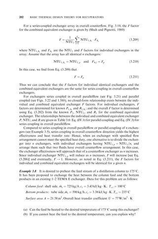


![TheMTDmethod is generally used for designing shell-and-tube exchangers because it
provides a ‘‘feel’’ to the designer regarding the size if the reduction in effective T (given
by Tm
Þ against the best possible T (given by Tlm
Þ for the counterflow exchanger.
A large reduction in Tm over Tlm means a low value of F or a large value of NTU
[see Eq. (3.200) or (3.204)] for the same counterflow effectiveness or NTUcf, or a reduc-tion
in the temperature effectiveness for the same NTU [see Eq. (3.203) or (3.204)]. In
such a case, the exchanger operates in the asymptotic region of the -NTU or P-NTU
curve; and a large increase in surface area provides only a small increase in heat transfer.
This is true in general regardless of whether or not there is a temperature cross for a
specified exchanger flow arrangement. Because the capital cost for a shell-and-tube
exchanger is an important design consideration, generally it is designed in the steep
region of the -NTU or P-NTU curve ð 60%Þ; and as a rule of thumb, the F value
selected is 0.80 and higher. However, a better guideline for Fmin is provided by Eq. (3.114)
when the temperature meet is at the end of the second tube pass in a 1–2 TEMA E
exchanger. Further detailed comparisons between the MTD and -NTU methods are
provided in Section 3.9.
When the temperatures of the hot and cold fluids remain constant (as in a phase-change
condition or C* ¼ 0) in a heat exchanger, Eqs. (3.182) and (3.183) become
Tm
¼ Tlm
¼ Th;i
Tc;i
¼ ITD ¼ Tmax and F ¼ 1 ð3:187Þ
This is also a good approximation when condensation takes place on one fluid side and
evaporation on the other fluid side (with each fluid side having a single component or an
azeotropic fluid), or one of the fluids can be water or other liquids with a high heat
capacity rate and having a high flow rate. In this case, Eq. (3.179) becomes
q ¼ UATm
¼ UA ðTh;i
Tc;i
Þ ¼ ðUAÞ
mod
ðTh;i
Tc;i
Þ ð3:188Þ
where is defined by Eq. (3.212). Here (UA)mod
¼ UA when the hot and cold fluid
temperatures are truly constant. However, when they are not constant, sometimes in
the literature ðUAÞ
mod
¼ UA is used to take into account the nonconstancy of the mean
temperature difference. Since the MTD method is more commonly used than the -P
method (discussed in Section 3.10), it is suggested Eq. (3.184) be used in all cases.
3.8 F FACTORS FOR VARIOUS FLOW ARRANGEMENTS
3.8.1 Counterflow Exchanger
We derive an expression for Tm and hence for F for the counterflow exchanger of Fig.
3.6. Following the same algebraic details starting from Eq. (3.68), and integrating Eq.
(3.75) from the hot-fluid inlet (section I) to outlet (section II), we get
ln
TII
TI
¼ 1
Cc
1
Ch
UA
ð3:189Þ
for constant U. Note that TI
¼ Th;i
Tc;o represents the temperature difference at one
end and TII
¼ Th;o
Tc;i at the other end. Replacing Cc and Ch of this equation by the
values obtained from the energy balances of Eq. (3.5), we get
ln
TII
TI
¼ 1
q
½ðTc;o
Tc;i
Þ ðTh;i
Th;o
ÞUA ¼ 1
q
ðTII
TI
ÞUA ð3:190Þ
190 BASIC THERMAL DESIGN THEORY FOR RECUPERATORS](https://image.slidesharecdn.com/fundamentalsofheatexchangerdesign-131001160835-phpapp01-141008073824-conversion-gate02/85/Fundamentalsofheatexchangerdesign-131001160835-phpapp01-239-320.jpg)


![F FACTORS FOR VARIOUS FLOW ARRANGEMENTS 193
Using the relationships of Eqs. (3.99), (3.103), and (3.108), F of Eq. (3.202) can be
expressed as a function of , NTU, and C*:
F ¼
ln½ð1 C*Þ=ð1 Þ
NTUð1 C*Þ for C*6¼ 1
NTUð1 Þ for C* ¼ 1
8
:
ð3:205Þ
Let us emphasize the interpretation of Eqs. (3.200) and (3.202). Since these equations
are based on the premises that P1
¼ P1;cf, R1
¼ R1;cf, and Tmax
¼ Tmax;cf, it means
that to achieve the same counterflow effectiveness for a given exchanger, we have
F NTU1
¼ NTU1;cf; thus the lower the value of the F factor, the higher will be the
required NTU1.
F / 1
NTU1
ð3:206Þ
Also, since F Tlm
¼ Tm
¼ ðTlm
Þ
cf, and F 1 for a noncounterflow exchanger, the
log-mean temperature difference for all other exchanger flow arrangements will be higher
than that for a counterflow exchanger for specified values of NTU1 and R1.
However, if we want to compare a given exchanger A to any other exchanger B (e.g.,
TEMA E vs. TEMA J) at the same NTU1, R1, and Tmax, we obtain the ratio FA=FB for
the two exchangers using Eq. (3.202) twice (in the ratio form):
FA
FB
¼
ln½ð1 R1P1;A
Þ=ð1 PÞ
1;A
Þ
ln½ð1 R1P1;B
Þ=ð1 PÞ
1;B
Þ for R1
6¼ 1
P1;A
ð1 P1;B
Þ
P1;B
ð1 P1;A
Þ for R1
¼ 1
8
:
ð3:207Þ
Here the second subscript A or B of P denotes the exchanger A or B, respectively. From
this equation it can be shown that for given values of NTU1, R1, and Tmax, we get
FA FB if P1;A P1;B
ð3:208Þ
This means that a reduction in F translates into a reduction in P1 and vice versa, when
comparing two exchangers at the same NTU1, R1, and Tmax.
Although F in Eq. (3.202) is a function of three nondimensional groups P1, R1, and
NTU1, we know that NTU1 is a function of P1 and R1, as can be found from Eq. (3.110).
Thus, F is a function of only two independent nondimensional groups, P1 and R1 [as
noted in Eq. (3.185)], P1 and NTU1, or NTU1 and R1, for a given flow arrangement.
Based on the results of Table 3.6, P1 can be presented explicitly as a function of NTU1
and R1 for all flow arrangements considered. However, NTU1 can be presented explicitly
as a function of P1 and R1 for only a few flow arrangements, as shown in Table 3.4 in
terms of the -NTU method. Hence, the NTU1 expression for these flow arrangements
can be substituted in Eq. (3.204) to obtain F as an explicit function of P1 and R1, or and
C*. All known explicit formulas for the F factor are presented in Table 3.8. For all other
flow arrangements of Table 3.6, since NTU1 cannot be expressed explicitly as a function](https://image.slidesharecdn.com/fundamentalsofheatexchangerdesign-131001160835-phpapp01-141008073824-conversion-gate02/85/Fundamentalsofheatexchangerdesign-131001160835-phpapp01-242-320.jpg)


![F FACTORS FOR VARIOUS FLOW ARRANGEMENTS 201
This rating problem can be made guaranteed convergent using the Newton–Raphson
method [i.e., the solution of f ðxÞ ¼ 0 where the function f is nonlinear in the present
case] as follows. Since
F ¼ 1
ðPs;Rs
Þ ¼ 2
ðTs;o
Þ ð1Þ
for this particular problem, and from the overall energy balance between the shell fluid
and tube fluid, we get for given Ps and Rs
Tt;o
¼ 3
ðTs;o
Þ ð2Þ
Hence,
Tlm
¼ 4
ðTs;o;Tt;o
Þ ¼ 5
ðTs;o
Þ ð3Þ
Thus, using the functional relationship of F and Tlm with Ts;o, we obtain the following
functional relationship for q from Eq. (3.184):
q ¼ UAF Tlm
¼ UA2
ðTs;o
Þ5
ðTs;o
Þ ¼ 6
ðTs;o
Þ ð4Þ
Since
q ¼ UAF Tlm
¼ Cs
ðTs;i
Ts;o
Þ ð5Þ
Hence,
UAF Tlm
Cs
ðTs;i
Ts;o
Þ ¼ 0 ¼ 6
ðTs;o
Þ 7
ðTs;o
Þ ¼ ðTs;o
Þ ð6Þ
In Eq. (6), the only unknown is Ts;o; which can be determined accurately by the Newton–
Raphson method of solving the f ðxÞ ¼ 0 equation. Subsequently, Tt;o can be computed
from the energy balance.
Discussion and Comments: This example clearly demonstrates that the rating problem
may not converge by the simple iterative scheme on Ps. It will converge slowly by
iterating on F. One may resort to a more complex numerical convergence scheme for a
guaranteed convergence. However, this problem can be solved relatively straightforward
by the P-NTU or -NTU method, as shown in Example 3.2 for counterflow and parallel-flow
arrangements with different operating conditions.
3.8.4 Heat Exchanger Arrays and Multipassing
We consider two cases: (1) determine the F factor for an exchanger array consisting of n
identical or nonidentical exchangers, and (2) determine the F factors for an exchanger
array for specified performance data (i.e., a combined equivalent exchanger), when the
number n of identical individual exchangers is increased so that individual NTU1=n
decreases (where NTU1 is for the combined equivalent exchanger). As we discussed in
Section 3.6.2, our description of an exchanger array also applies to a multipass exchanger
having n passes.](https://image.slidesharecdn.com/fundamentalsofheatexchangerdesign-131001160835-phpapp01-141008073824-conversion-gate02/85/Fundamentalsofheatexchangerdesign-131001160835-phpapp01-250-320.jpg)
![202 BASIC THERMAL DESIGN THEORY FOR RECUPERATORS
For a series-coupled exchanger array in overall counterflow, Fig. 3.19, the F factor
for the combined equivalent exchanger is given by (Shah and Pignotti, 1989)
F ¼ 1
NTU1
n
X
i¼1
NTU1;Ai
FAi
ð3:209Þ
where NTU1;Ai and FAi are the NTU1 and F factors for individual exchangers in the
array. Assume that the array has all identical n exchangers:
NTU1;Ai
¼ NTU1; p and FA;i
¼ Fp
ð3:210Þ
In this case, we find from Eq. (3.209) that
F ¼ Fp
ð3:211Þ
Thus we can conclude that the F factors for individual identical exchangers and the
combined equivalent exchangers are the same for series coupling in overall counterflow
exchangers.
For exchangers series coupled in overall parallelflow (see Fig. 3.21) and parallel
coupled (see Figs. 3.22 and 1.58b), no closed-form relationship exists between the indi-vidual
and combined equivalent exchanger F factors. For individual exchangers, F
factors are determined for known P1;Ai and R1;Ai ; and the overall F factor is determined
using Eq. (3.202) from the known P1, NTU1, and R1 for the combined equivalent
exchanger. The relationships between the individual and combined equivalent exchanger
P, NTU, and R are given in Table 3.6: Eq. (IV.1) for parallel coupling and Eq. (IV.3) for
series coupling in overall parallelflow.
Compared to series coupling in overall parallelflow or parallel coupling of n exchan-gers
(see Example 3.5), series coupling in overall counterflow direction yields the highest
effectiveness and heat transfer rate. Hence, when an exchanger with specified flow
arrangement cannot meet the specified heat duty, one alternative is to divide the exchan-ger
into n exchangers, with individual exchangers having NTU1; p
¼ NTU1=n, and
arrange them such that two fluids have overall counterflow arrangement. In this case,
the exchanger effectiveness will approach that of a counterflow exchanger as n increases.
Since individual exchanger NTU1; p will reduce as n increases, F will increase [see Eq.
(3.206)] and eventually, F ! 1. However, as noted in Eq. (3.211), the F factors for
individual and combined equivalent exchangers will be identical for a given n.
Example 3.8 It is desired to preheat the feed stream of a distillation column to 1758C.
It has been proposed to exchange the heat between the column feed and the bottom
products in an existing 1–2 TEMA E exchanger. Data for this problem are as follows:
Column feed : shell side; m_ s
¼ 725 kg=h; cs
¼ 3:43 kJ=kg K; Ts;i
¼ 1008C
Bottom products : tube side;m_ t
¼ 590 kg=h; ct
¼ 3:38 kJ=kg K;Tt;i
¼ 2358C
Surface area A ¼ 21:58m2; Overall heat transfer coefficient U ¼ 77W=m2 K
(a) Can the feed be heated to the desired temperature of 1758C using this exchanger?
(b) If you cannot heat the feed to the desired temperature, can you explain why?](https://image.slidesharecdn.com/fundamentalsofheatexchangerdesign-131001160835-phpapp01-141008073824-conversion-gate02/85/Fundamentalsofheatexchangerdesign-131001160835-phpapp01-251-320.jpg)


![F FACTORS FOR VARIOUS FLOW ARRANGEMENTS 205
(b) The F factor for this case is 0.5023 from Eq. (III.1.3) of Table 3.6 or extrapolation
in Fig. 3.26 for P1
¼ 0:5108 and R1
¼ 1:247. It is too low and there is a temperature cross
(see Fmin line in Fig. 3.26). The exchanger flow arrangement is just not efficient to heat the
feed to 1758C with the surface area provided or even increasing A to 1.
(c) Now NTU1; p
¼ 2:406=2 ¼ 1:203, and R1
¼ 1:247. Hence, P1; p
¼ 0:4553 from Eq.
(III.1.1) of Table 3.6 or 0.46 from Fig. 3.13. The overall effectiveness of two 1–2 exchan-gers
in overall counterflow arrangement is determined from Eq. (3.131).
P1
¼
½ð1 R1P1; p
Þ=ð1 P1; p
Þ2 1
½ð1 R1P1; p
Þ=ð1 P1; p
Þ2 R1
¼
½ð1 1:247 0:4553Þ=ð1 0:4553Þ2 1
½ð1 1:247 0:4553Þ=ð1 0:4553Þ2 1:247
¼ 0:5999
Ts;o
¼ Ts;i
þ P1
ðTt;i
Ts;i
Þ ¼ 1008C þ 0:5999ð235 100Þ8C ¼ 181:08C
Tt;o
¼ Tt;i
P1R1
ðTt;i
Ts;i
Þ ¼ 2358C 0:5999 1:247ð235 100Þ8C ¼ 134:08C
Using two exchangers, the feed can be heated to 1818C, which is above the required value
of 1758C. Ans.
(d) Instead of one 1–2 exchanger having NTU1
¼ 2:406, if we employ two 1–2 exchan-gers
in series in overall counterflow direction each having NTU1
¼ 1:203, we can increase
the shell fluid temperature effectiveness from 0.5108 to 0.5999. Regardless of the flow
arrangement of individual heat exchangers, when two or more exchangers are connected
in series in the overall counterflow direction, the overall temperature effectiveness
approaches that of a pure counterflow exchanger. Note that in the present problem,
part (c), F ¼ 0:7786 for P1; ¼ p
0:4553 and R1
¼ 1:247 using Eq. (III.1.3) of Table 3.6
(or see Fig. 3.26). Hence, there is only a small temperature cross in individual exchangers,
and the surface is used more efficiently.
Note that by making two smaller frontal area 1–2 exchangers, the flow velocities will
go up by a factor of 2, due to the reduction in flow area by one-half. This change will also
increase individual h’s and hence further increase in NTU1, P1, and q than what is
calculated. An important but negative impact of this design will be a significant increase
in the pressure drop on both sides (discussed further in Chapter 6).
(e) The F factor for the original 1–2 exchanger for NTU1
¼ 2:406 and R1
¼ 1:247 is
0.5023, as noted in part (b). When two 1–2 exchangers are connected in overall counter-flow
direction, the F factor for the two exchangers in series is the same as the F factor for
the individual exchangers [see Eq. (3.211)], since F ¼ 1 for counterflow arrangement.
Hence, for two 1–2 exchangers in series, F ¼ 0:7786 for NTU1; ¼ p
1:203 and R1
¼ 1:247
from Eq. (III.1.3) of Table 3.6 or Fig. 3.26.
An alternative proof can be presented from the general definition of the F factor of
Eq. (3.204) as follows.
F ¼ TmaxP1
NTU1 Tlm
This F formula is valid for one exchanger or multiple exchangers in series in overall
counterflow direction as long as the appropriate values of P1, NTU1, and Tlm are used.
For two exchangers in series, total NTU1
¼ 2:406 and P1
¼ 0:5999, as calculated in
part (c), Tmax
¼ 2358C 1008C ¼ 1358C, and Tlm
¼ 43:238C is calculated from the
temperatures found in part (c).](https://image.slidesharecdn.com/fundamentalsofheatexchangerdesign-131001160835-phpapp01-141008073824-conversion-gate02/85/Fundamentalsofheatexchangerdesign-131001160835-phpapp01-254-320.jpg)


![216 BASIC THERMAL DESIGN THEORY FOR RECUPERATORS
Most of the configurations of Table 3.6 are geometrically symmetric (i.e., after
reversal of both fluids, they coincide with the original geometry, except for some trivial
transformation, such as rotation, mirror image, etc.). For such cases, flow reversal sym-metry
does not provide any additional information. The geometrically asymmetric cases
are III.1, III.2, III.4, III.10, III.11, III.12, V.3, V.6, V.11, V.12, and V.13 in Table 3.6. For
these cases, two seemingly different geometries (one shown in the schematics of Table 3.6
and the other with both flows reversed) have the same effectiveness; and hence the
effectiveness of the seemingly different configuration is known instantly through the
concept of flow reversibility.
3.11.7 Rules for the Determination of Exchanger Effectiveness with One Fluid Mixed
As presented in Section 3.11.6, the principle of flow reversibility indicates that when the
directions of both fluids are reversed in any two-fluid individual exchangers (not an
array), the exchanger effectiveness (and P1 and F) does not change. In contrast, con-sider
a multipass or complex configuration exchanger having at least one fluid side
perfectly mixed throughout, the other fluid side being mixed, unmixed, or partially
mixed. If the effectiveness of such an exchanger is known for overall parallelflow (or
counterflow), the effectiveness of the same exchanger configuration with the direction of
only one fluid (which one is immaterial) reversed [i.e., the resulting overall counterflow
(parallelflow)], can be found readily as follows. The effectiveness P1 of the original
exchanger and the effectiveness ^ P1 of the exchanger with one fluid reversed are related
as follows (Sekulic´ et al., 1999):
^ P1
ðR1;NTU1
Þ ¼ P1
ðR1;NTU1
Þ
1 þ R1P1
ðR2;NTU1
Þ
ð3:216Þ
Here the subscript 1 refers to the fluid side having no restrictions (i.e., it can be mixed,
unmixed, or split). The temperature effectiveness of the mixed fluid (the subscript 2) is
then given by
^ P2
ðR2;NTU2
Þ ¼
P2
ðR2;NTU2
Þ
1 P1
ðR2;NTU2
Þ
ð3:217Þ
It must be emphasized that Eq. (3.216) or (3.217) is a mathematical relationship
between values of P of the original and inverted exchangers. ^ P of the inverted exchanger
for the physical (positive) values of R is related to P of the original exchanger for the
unphysical (negative) values of R as shown in Eq. (3.216) or (3.217).
If one of the fluid flow directions is reversed for the exchangers of Eqs. (III.3), (III.7),
and (III.9), Eq. (3.216) can be applied to get the effectiveness of the overall parallelflow
exchanger, and hence those configurations are not included in Table 3.6.
3.12 HEAT EXCHANGER DESIGN PROBLEMS
While comparing the -NTU and MTD methods in Section 3.9, the solution procedures
for two heat exchanger design problems (rating and sizing) were provided. However,
considering seven variables of the heat exchanger design problem [Eq. (3.7)], there are a
total of 21 problems, as shown in Table 3.11. In this table, the dimensionless parameters](https://image.slidesharecdn.com/fundamentalsofheatexchangerdesign-131001160835-phpapp01-141008073824-conversion-gate02/85/Fundamentalsofheatexchangerdesign-131001160835-phpapp01-265-320.jpg)


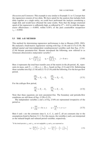


![218 BASIC THERMAL DESIGN THEORY FOR RECUPERATORS
are also included with known or unknown values based on the dimensional variables. If
only one of the temperatures is known, we evaluate the specific heat at that temperature
for the determination/estimate of C and hence R; eventually, once we know both tem-peratures,
an iteration may be needed. If specific heats are treated as constant, C1 and C2
in the equations above are interchangeable with m_ 1 and m_ 2. Also, we have presently
considered the UA product as one of the design parameters. We discuss separating U and
A when we discuss the detailed sizing problem in Chapter 9. In the foregoing count, we
have not added q since q can readily be calculated from the overall energy balance [Eq.
(3.5)] or the rate equation [Eq. (3.6) or (3.12)]. Alternatively, if q is given, one of the
temperatures or the flow rates (heat capacity rate) could be unknown in Table 3.11. We
could classify the first six problems as variations of the sizing problem and the next 15
problems as a variation of the rating problem. Using the P-NTU method, these 21
problems can be solved as follows.
1. For problems 1 to 6, P1 (also P2) and R1 are known through the heat balance.
Hence, NTU1 can be calculated from the P-NTU formula for a given flow arrange-ment,
either straightforward or iteratively, depending on whether NTU can be
expressed explicitly (see Table 3.4) or implicitly (see Table 3.6).
2. For problem 7, since all four temperatures are known, both P1 and R1 are known
through their definitions [Eqs. (3.96) and (3.105)]. Hence, NTU1 can be calculated
as mentioned in the preceding paragraph for a given flow arrangement. Then
C1
¼ UA=NTU1 and C2
¼ C1=R1. Knowing the specific heats of the given fluids,
one can determine m_ 1 and m_ 2.
3. For problems 8 to 13, NTU1 and R1 are known. Hence, determine P1 using the
appropriate formula from Table 3.6. Now knowing P1, R1, and the definition of
P1, compute the unknown temperatures using the formulas given in Table 3.10.
4. Problems 14 and 16 can only be solved iteratively, with the solution procedure
for problem 14 as follows. Assume m_ 1 (or C1). Calculate R2
ð¼ C2=C1
Þ. From the
problem specifications, NTU2
¼ UA=C2 and q ¼ C2
jT2;i
T2;o
j are known.
Hence, knowing NTU2 and R2 for a given flow arrangement, determine P2
using the appropriate formula from Table 3.6. Subsequently, compute T1;i from
the definition of P2, and C1 from the energy balance C1
jðT1;i
T1;o
Þj ¼ q. With
this new value of C1, repeat all the calculations above. Continue to iterate until the
successive values of C1 converge within the accuracy desired. The solution pro-cedure
for problem 16 is identical to that for problem 14 just described, starting
with assuming m_ 2 (or C2) and computing R1 and NTU1. The solution procedure
for problem 15 is relatively straightforward. In this case, P2 and NTU2 are given.
From the known P-NTU formula from Table 3.6, compute R2 iteratively (such
as using the Newton–Raphson method) since it is an implicit function of P2 and
NTU2. Similarly, P1 and NTU1 are known for problem 17 and determine
iteratively R1 from the known P-NTU formula of Table 3.6.
5. Problems 18 and 20 can only be solved iteratively, with the solution procedure for
problem 18 as follows. Assume C2 and hence determine R1
ð¼ C1=C2
Þ. Also,
compute NTU1
ð¼ UA=C1
Þ from the input. For a given flow arrangement, deter-mine
P1 using the appropriate formula from Table 3.6. Subsequently, compute T1;i
from the definition of P1. Finally, calculate C2 from the overall energy balance
C1
ðT1; T1;Þ ¼ Þ. i
o
C2
ðT2;o
T2;i
With this new value of C2, repeat all the calcula-tions
above. Continue to iterate until successive values of C2 converge within the](https://image.slidesharecdn.com/fundamentalsofheatexchangerdesign-131001160835-phpapp01-141008073824-conversion-gate02/85/Fundamentalsofheatexchangerdesign-131001160835-phpapp01-372-320.jpg)
![SUMMARY 219
desired accuracy. The solution procedures for problem 20 is identical to that for
problem 18 just described, starting with assuming C1 and computing R2 and
NTU2.
The solution procedure for problem 19 is relatively straightforward. In this case,
P2 and NTU1 are known. For the given flow arrangement, select the P1-NTU1
formula from Table 3.6 and replace P1 by P2=R1 [see Eq. (3.98)]. The resulting
equation has only one unknown, R1, since NTU1 and P2 are known; and R1 is
implicit. It can be computed iteratively using, for example, the Newton–Raphson
method. Similarly, P1 and NTU2 are known in problem 21, and compute R2
iteratively after replacing P1 by P2R2 in the appropriate P-NTU formula of
Table 3.6. See the footnote of Table 3.6 for how to convert P1-NTU1-R1 formulas
into P2-NTU2-R2 formulas.
SUMMARY
This chapter is very important to the book. We have presented in considerable detail the
basic thermal design theory for recuperators or exchangers with no moving parts or
periodic flows as in regenerators. Through the problem formulations, it is shown that
there are six independent and one or more dependent variables for the exchanger thermal
design problem for any flow arrangement. The solution to this problem can be presented
in terms of -NTU, P-NTU, MTD, -P and P1-P2 methods. The exchanger rating or
sizing problem can be solved by any of these methods and will yield the identical solution
within the numerical error of computation. Theoretical details are presented for the -
NTU, P-NTU, and MTD methods in the text for an understanding of concepts, these
methods, and their advantages and disadvantages. Many idealizations are made to
simplify the complex heat exchanger design problem to obtain the solution in terms of
-NTU, P-NTU, and MTD parameters. A thorough understanding of the concepts and
results presented in this chapter will provide a strong foundation for rating, sizing, and
analysis of industrial heat exchangers.
REFERENCES
Bacˇ lic´ , B. S., 1990, -Ntu analysis of complicated flow arrangements, in Compact Heat Exchangers:
A Festschrift for A. L. London, R. K. Shah, A. D. Kraus, and D. Metzger, eds., Hemisphere
Publishing, Washington, DC, pp. 31–90.
Bell, K. J., 1998, Approximate sizing of shell-and-tube heat exchangers, in Heat Exchanger Design
Handbook, G. F. Hewitt, exec. ed., Begell House, New York, Vol. 3, Sec. 3.1.4.
Kandlikar, S. G., and R. K. Shah, 1989, Asymptotic effectiveness–NTU formulas for multipass
plate heat exchangers, ASME J. Heat Transfer, Vol. 111, pp. 314–321.
McAdams, W. H., 1954, Heat Transmission, 3rd ed., McGraw-Hill, New York, pp. 129–131.
Mueller, A. C., 1967, New Charts for True Mean Temperature Difference in Heat Exchangers, AIChE
Paper 10, 9th National Heat Transfer Conf., Seattle, WA.
Pignotti, A., and G. O. Cordero, 1983, Mean temperature difference in multipass crossflow, ASME
J. Heat Transfer, Vol. 105, pp. 584–591.
Pignotti, A., and R. K. Shah, 1992, Effectiveness-number of transfer units relationships for heat
exchanger complex flow arrangements, Int. J. Heat Mass Transfer, Vol. 35, pp. 1275–1291.](https://image.slidesharecdn.com/fundamentalsofheatexchangerdesign-131001160835-phpapp01-141008073824-conversion-gate02/85/Fundamentalsofheatexchangerdesign-131001160835-phpapp01-373-320.jpg)


![230 BASIC THERMAL DESIGN THEORY FOR RECUPERATORS
3.15 Given Th;i
¼ 608C, Th;o
¼ 43:38C, Tc;i
¼ 26:78C, and Tc;o
¼ 40:68C, calculate the
true-mean temperature difference for (a) parallelflow, (b) counterflow, (c) single-pass
crossflow with both fluids unmixed, (d) single-pass crossflow with cold fluid
unmixed and hot fluid mixed, and (e) a 1–2 TEMA E exchanger. Also determine
the exchanger effectiveness for each case.
3.16 To calculate Tm for any flow arrangement (except for parallelflow), we calculate
it from
Tm
¼ F Tlm
where F is the correction factor applied to the logarithmic temperature difference
Tlm for a hypothetical (or actual) counterflow exchanger operating at the same R
and the same terminal temperatures. This Tlm is obtained from Eq. (3.172) using
Eq. (3.173). Now consider that we use the same counterflow Tlm definition for a
parallelflow exchanger [i.e., Eq. (3.172) in conjunction with Eq. (3.173) and not
Eq. (3.174)]. In this case, F will not be unity, but it will be
F ¼ R þ 1
R 1
ln½ð1 RPÞ=ð1 PÞ
ln½1 ð1 þ RÞP
Derive this equation for F for a parallelflow exchanger.
3.17 Lubricating oil at a temperature of 608C enters a 10mm diameter tube with a
velocity of 2.0 m/s. The tube surface is maintained at 308C. Calculate the tube
length required to cool the oil to 458C. Consider the following properties for oil:
¼ 865 kg=m3, k ¼ 0:14W=m K, cp
¼ 1780 J=kg K, and ¼ 0:0078 Pa s.
For oil flow in the tube, the heat transfer coefficient h ¼ 51:2W=m2 K.
3.18 A shell-and tube exchanger is required to cool the hot oil from 2408C to 908C.
After some process, the same oil returns to the exchanger at 408C and leaves at
1908C. Assume a negligible change in the specific heat of oil in the temperature
range 110 to 1708C.
(a) If you design one 1–2 TEMA E shell-and-tube exchanger, would there be a
temperature cross?
(b) Is it possible to design one 1–2 TEMA E exchanger to meet the required
specifications, and why?
(c) What minimum number of 1–2 TEMA E exchangers in series would you
require to eliminate the temperature cross? Hint: Use an appropriate
equation from Eqs. (3.131)–(3.139). Specify any idealization you may
make.
(d) What would be the overall arrangement of two fluids in part (c)? Tell whether
or not you could use an alternate (opposite) flow arrangement and why.
(e) What would be the F factor for part (c)?
3.19 Two identical single-pass counterflow exchangers are used for heating water
ðcp
¼ 4:2kJ=kg K) at 258C with the hot oil ðcp
¼ 2:1kJ=kg K) at 1208C. The
water and oil flow rates are 1 and 4 kg/s, respectively. The heat exchangers are
connected in series on the water side and in parallel on the oil side, as shown in](https://image.slidesharecdn.com/fundamentalsofheatexchangerdesign-131001160835-phpapp01-141008073824-conversion-gate02/85/Fundamentalsofheatexchangerdesign-131001160835-phpapp01-384-320.jpg)


![LONGITUDINAL WALL HEAT CONDUCTION EFFECTS 233
tion in the wall and in fluids from the hotter to colder temperature regions, which may
affect the heat transfer rate from the hot fluid to the cold fluid.
Heat conduction in a fluid in the fluid flow direction is negligible for Pe 10 and
x* 0:005, where the Pe´ clet number Pe ¼ Re Pr ¼ umDh= and x* ¼ x=ðDh
PeÞ; the
significance and meaning of Pe and x* are presented in Section 7.2. For most heat
exchangers, except liquid metal heat exchangers, Pe and x* are higher than the values
indicated above. Hence, longitudinal heat conduction in the fluid is negligible in most
applications and is not covered here.
If a temperature gradient is established in the separating walls between fluid flow
streams in a heat exchanger, heat transfer by conduction takes place from the hotter
to colder region of the wall, flattens the wall temperature distribution, and reduces the
performance of the exchanger. For example, let us review typical temperature distribu-tions
in the hot fluid, cold fluid, and wall for a counterflow heat exchanger as shown in
Fig. 4.1. Dashed lines represent the case of zero longitudinal heat conduction, and solid
lines represent the case of finite longitudinal conduction [ ¼ 0:4, defined in Eq. (4.13)].
From the figure it is clear that longitudinal conduction in the wall flattens the tempera-ture
distributions, reduces the mean outlet temperature of the cold fluid, and thus reduces
the exchanger effectiveness from 90.9% to 73.1%. This in turn produces a penalty in the
exchanger overall heat transfer rate. The reduction in the exchanger effectiveness at a
specified NTU may be quite significant in a single-pass exchanger having very steep
temperature changes in the flow direction (i.e., large Th=L or Tc=L). Such a situation
arises for a compact exchanger designed for high effectiveness (approximately above
80%) and has a short flow length L. Shell-and-tube exchangers are usually designed
for an exchanger effectiveness of 60% or below per pass. The influence of heat conduc-tion
in the wall in the flow direction is negligible for such effectiveness.
Since the longitudinal wall heat conduction effect is important only for high-effec-tiveness
single-pass compact heat exchangers, and since such exchangers are usually
designed using -NTU theory, we present the theory for the longitudinal conduction
effect by an extension of -NTU theory. No such extension is available in the MTD
method.
The magnitude of longitudinal heat conduction in the wall depends on the wall heat
conductance and the wall temperature gradient. The latter in turn depends on the
thermal conductance on each side of the wall. To arrive at additional nondimensional
groups for longitudinal conduction effects, we can work with the differential energy and
rate equations of the problem and can derive the same Eq. (4.9) mentioned later. For
example, see Section 5.4 for the derivation of appropriate equations for a rotary regen-erator.
However, to provide a ‘‘feel’’ to the reader, a more heuristic approach is followed
here. Let us consider the simple case of a linear temperature gradient in the wall as shown
in Fig. 4.1. The longitudinal conduction rate is
qk
¼ kwAk
Tw;1
Tw;2
L
ð4:1Þ
where Ak is total wall cross-sectional area for longitudinal conduction. The convective
heat transfer from the hot fluid to the wall results in its enthalpy rate drop as follows,
which is the same as enthalpy rate change (convection rate) qh:
ðm_ hÞ
h
¼ Ch
ðTh;1
Th;2
Þ ¼ qh
ð4:2Þ](https://image.slidesharecdn.com/fundamentalsofheatexchangerdesign-131001160835-phpapp01-141008073824-conversion-gate02/85/Fundamentalsofheatexchangerdesign-131001160835-phpapp01-387-320.jpg)


![236 ADDITIONAL CONSIDERATIONS FOR THERMAL DESIGN OF RECUPERATORS
one of them, alternatively, a unique longitudinal conduction parameter is defined as
follows for a counterflow exchanger:
¼ kwAk
LCmin
ð4:13Þ
and Eq. (4.9) takes the following form for a counterflow exchanger:
¼ NTU;C*; ; o ½ ð hAÞ* ð4:14Þ
However, for exchangers other than counterflow and parallelflow, Eq. (4.9) is the correct
general relationship.
Multiplying by (Th;i
Tc;i) the numerator and denominator of Eq. (4.13), can be
interpreted as the ratio of longitudinal heat conduction rate in a counterflow heat
exchanger (having NTU¼1and C* ¼ 1) to the thermodynamically maximum possible
heat transfer rate.
Next, we summarize the longitudinal conduction effects for various exchangers.
4.1.1 Exchangers with C* ¼ 0
The operating condition having C* ¼ 0 usually occurs when condensing or boiling takes
place on one side of a two-fluid heat exchanger. The thermal resistance (1/hA) in such a
case on the two-phase (Cmax) side is generally very small, and hence the wall temperature
is close to the fluid temperature of the Cmax side and almost constant (i.e., the wall has a
very small temperature gradient, if any, in the longitudinal direction). As a result, long-itudinal
heat conduction in the wall is negligible and its effect on the exchanger effec-tiveness
is also negligible for the C* ¼ 0 case.
4.1.2 Single-Pass Counterflow Exchanger
The counterflow exchanger problem with finite longitudinal wall conduction has been
analyzed by Kroeger (1967), among others, and extensive graphical results are available
for the exchanger ineffectiveness (1 ) for a wide range of NTU, C*, and . Kroeger
showed that the influence of (ohA)* on or (1 ) is negligible for 0:1 ðohAÞ* 10,
and hence the longitudinal wall conduction effect can be taken into account by only one
additional parameter [see Eq. (4.14)] besides NTU and C*. The penalty to exchanger
effectiveness due to longitudinal wall conduction increases with increasing values of
NTU, C*, and , and is largest for C* ¼ 1. Kroeger’s solution for C* ¼ 1 and
0:1 ðohAÞ* 10 is
¼ 1 1
1 þ NTUð1 þ Þ=ð1 þ NTUÞ
ð4:15Þ
where for NTU 3,
¼ NTU
1=2
1 þ NTU
ð4:16Þ](https://image.slidesharecdn.com/fundamentalsofheatexchangerdesign-131001160835-phpapp01-141008073824-conversion-gate02/85/Fundamentalsofheatexchangerdesign-131001160835-phpapp01-390-320.jpg)


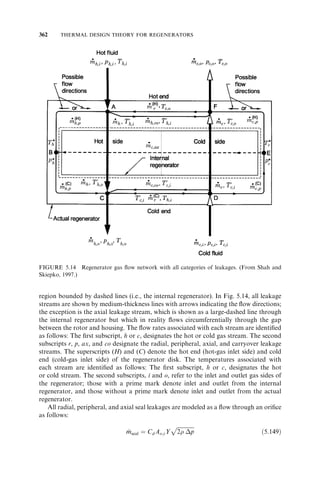


![NONUNIFORM OVERALL HEAT TRANSFER COEFFICIENTS 245
overall heat transfer coefficient is dependent on heat transfer surface geometry, indivi-dual
Nu (as a function of relevant parameters), thermal properties, fouling effects, tem-perature
variations, temperature difference variations, and so on. No information is
available on the effect of some of these parameters, and it is beyond the scope of this
book to discuss the effect of other parameters. In this section we concentrate on non-uniformities
in U due to temperature and length effects.
To outline how to take temperature and length effects into account, let us introduce
specific definitions of local and mean overall heat transfer coefficients. The local overall
heat transfer coefficient U x1 *
ð ; TÞ, is defined as follows in an exchanger at a local
; x2 *
position ½x* ¼ x=ðDh
Re PrÞ, subscripts 1 and 2 for fluids 1 and 2] having surface area
dA and local temperature difference ðTh
Tc
Þ ¼ T:
U ¼ dq
dA T
ð4:24Þ
Traditionally, the mean overall heat transfer coefficient Um
ðTÞ is defined as
1
UmA
¼ 1
ðohmAÞ
h
þ Rw
þ 1
ðohmAÞ
c
ð4:25Þ
Here fouling resistances and other resistances are not included for simplifying the dis-cussion
but can easily be included if desired in the same way as in Eq. (3.24). In Eq. (4.25),
the hm’s are the mean heat transfer coefficients obtained from the experimental/empirical
correlations, and hence represent the surface area average values. The experimental/
empirical correlations are generally constant fluid property correlations, as explained
in Section 7.5. If the temperature variations and subsequent fluid property variations are
not significant in the exchanger, the reference temperature T in Um
ðTÞ for fluid properties
is usually the arithmetic mean of inlet and outlet fluid temperatures on each fluid side for
determining individual hm’s; and in some cases, this reference temperature T is the log-mean
average temperature on one fluid side, as discussed in Section 9.1, or an integral-mean
average temperature. If the fluid property variations are significant on one or both
fluid sides, the foregoing approach is not adequate.
A more rigorous approach is the area averageU ^
used in the definition of NTU [see the
first equality in Eq. (3.59)], defined as follows:
U ^
¼ 1
A
ð
A
Uðx; yÞ dA ð4:26Þ
This definition takes into account exactly both the temperature and length effects for
counterflow and parallelflow exchangers, regardless of the size of the effects. However,
there may not be possible to have a closed-form expression for Uðx; yÞ for integration.
Also, no rigorous proof is available that Eq. (4.26) is exact for other exchanger flow
arrangements.
When both the temperature and length effects are not negligible, Eq. (4.24) needs to be
integrated to obtain an overall U (which takes into account the temperature and length
effects) that can be used in conventional heat exchanger design. The most accurate
approach is to integrate Eq. (4.24) numerically for a given problem. However, if we
can come up with some reasonably accurate value of the overall U after approximately](https://image.slidesharecdn.com/fundamentalsofheatexchangerdesign-131001160835-phpapp01-141008073824-conversion-gate02/85/Fundamentalsofheatexchangerdesign-131001160835-phpapp01-399-320.jpg)


![248 ADDITIONAL CONSIDERATIONS FOR THERMAL DESIGN OF RECUPERATORS
Now we discuss methods that take temperature and length effects into account, to
arrive at U for the exchanger analysis.
4.2.1 Temperature Effect
4.2.1.1 Counterflow Exchanger. Consider a single-pass counterflow exchanger in
which U varies linearly with the temperature of either fluid stream, U ¼ að1 þ bTÞ,
where a and b are constants. In this case, the mean value of U T (where T is the
temperature difference between the hot and cold fluids) is as given by Colburn (1933):
q
A
¼ ðU TÞ
m
¼ UI TII
UII TI
lnðUI TII=UII TI
Þ
ð4:36Þ
where UI and UII are overall heat transfer coefficients determined at the exchanger hot
and cold terminals, and TI and TII are given by Eq. (3.173). Note that ðU TÞ
m
cannot be equal to U~ Tm. In this case, from Eq. (4.36), we get the exchanger heat
transfer rate as q ¼ ðU TÞ
mA. Equation (4.36) represents a good approximation for
very viscous liquids and partial condensation, and further discussion will be provided
later with an example.
An alternative approach to take into account the temperature effect on U is to use the
approximate method of integration by evaluating local U at specific points in the exchan-ger
or perform a numerical analysis. Since such methods are more general, they are
discussed next for all other exchanger flow arrangements.
4.2.1.2 Other Exchangers. We first illustrate the concept of how to include the effect
of variable UA for a counterflow exchanger and then extend it to all other flow arrange-ments.
To find out whether or not variations in UA are significant with temperature
variations, first evaluate UA at the two ends of a counterflow exchanger or a hypo-thetical
counterflow for all other exchanger flow arrangements. If it is determined that
variations in UA are significant, such as shown in Fig. 4.4, the average value U~A can be
determined by approximate integration of the variations in UA [i.e., Eq. (4.29) with the
first equality sign], by the three-point Simpson method as follows (Roetzel and Spang,
1993):
1
U~A
¼ 1
6
1
UIA
þ 2
3
1
U1=2 * A
þ 1
6
1
UIIA
ð4:37Þ
where
=2A ¼ U1=2A
U*1
T1=2
T*1
=2
ð4:38Þ
In Eq. (4.38), T1=2 and T*1
=2 are defined as
T1=2
¼ Th;1=2
Tc;1=2 and T*1=2
ð Þ1=2 ð4:39Þ
¼ TI TII](https://image.slidesharecdn.com/fundamentalsofheatexchangerdesign-131001160835-phpapp01-141008073824-conversion-gate02/85/Fundamentalsofheatexchangerdesign-131001160835-phpapp01-402-320.jpg)
![NONUNIFORM OVERALL HEAT TRANSFER COEFFICIENTS 249
FIGURE 4.4 Variable UA in a counterflow exchanger for the Simpson method.
where the subscripts I and II correspond to terminal points at the end sections, and the
subscript 1
2 corresponds to a point in between defined by the second equation, respec-tively.
Here Th;1=2 and Tc;1=2 are computed through the procedure of Eqs. (4.43)–(4.45).
Usually, uncertainty in the individual heat transfer coefficient is high, so that the
three-point approximation may be sufficient in most cases. Note that for simplicity, we
have selected the third point as the middle point in the example above. The middle point
is defined in terms of TI and TII [defined by Eq. (3.173)] to take the temperature effect
properly into account; it is not a physical middle point along the length of the exchanger.
The step-by-step procedure that involves this approach is presented in Section 4.2.3.1.
4.2.2 Length Effect
The heat transfer coefficient can vary significantly in the entrance region of laminar flow.
This effect is negligible for turbulent flows. Hence, we associate the length effect to
laminar flow. For hydrodynamically developed and thermally developing flow, the
local and mean heat transfer coefficients hx and hm for a circular tube or parallel plates
are related as follows (Shah and London, 1978):
hx
¼ 2
3 hm
ðx*Þ1=3 ð4:40Þ
where x* ¼ x=ðDh
Re PrÞ. Using this variation in h on one or both fluid sides, counter-flow
and crossflow exchangers have been analyzed, and the correction factors are
presented in Fig. 4.5 and Table 4.3 as a function of ’1 or ’2, where
’1
¼ o;2hm;2A2
1
o;1hm;1A1
þ 2Rw
’2
¼ Rw
1
ðohmAÞ
1
þ 1
ohm ð AÞ
2
1
ð4:41Þ
The value of is 0.89 for ’1
¼ 1, (i.e., when the exchanger has the hot- and cold-side
thermal resistances approximately balanced and Rw
¼ 0). Thus, when a variation in the
heat transfer coefficient due to the thermal entry length effect is considered,U U~ or Um
since U ¼ U~ from Eq. (4.34). This can be explained easily if one considers the thermal
resistances connected in series for the problem. For example, consider a very simplified
problem with the heat transfer coefficient on each fluid side of a counterflow exchanger](https://image.slidesharecdn.com/fundamentalsofheatexchangerdesign-131001160835-phpapp01-141008073824-conversion-gate02/85/Fundamentalsofheatexchangerdesign-131001160835-phpapp01-403-320.jpg)

![NONUNIFORM OVERALL HEAT TRANSFER COEFFICIENTS 251
4.2.3 Combined Effect
A specific step-by-step procedure is presented below to take into account the combined
temperature and length effects on U; the reader may refer to Shah and Sekulic´ (1998) for
further details. First, we need to determine heat transfer coefficients on each fluid side by
taking into account fluid property variations due to two effects: (1) distortion of velocity
and temperature profiles at a given flow cross section due to fluid property variations,
and (2) variations in fluid temperature along the axial and transverse directions in the
exchanger. In general, most correlations for the heat transfer coefficient are derived
experimentally at almost constant fluid properties (because generally, small temperature
differences are maintained during experiments) or are theoretically/numerically obtained
for constant fluid properties. When temperature differences between the fluid and wall
(heat transfer surface) are large, the fluid properties will vary considerably across a given
cross section (at a local x) and will distort both velocity and temperature profiles. In that
case, the dilemma is whether to use the fluid bulk temperature, wall temperature, or
something in between for fluid properties to determine h’s for constant property correla-tions.
Unless a specific heat transfer correlation includes this effect, it is commonly taken
into account by a property ratio method using both fluid bulk temperatures and wall
temperature, as discussed in Section 7.6. Hence, it must be emphasized that the local heat
transfer coefficients at specific points needed in the Simpson method of integration must
first be corrected for the local velocity and temperature profile distortions by the property
ratio method and then used as local h values for the integration. The net effect on U~ due
to these two temperature effects can be significant, and U~ can be considerably higher or
lower than Um at constant properties.
The individual heat transfer coefficients in the thermal entrance region could be
generally high. However, in general it will have less impact on the overall heat transfer
coefficient. This is because when computing Ulocal by Eq. (4.25), with Um and hm’s
replaced by corresponding local values [see also Eq. (3.20) and the subsequent discus-sion],
its impact will be diminished, due to the presence of the other thermal resistances in
the series that are controlling (i.e., having a low hA value). It can also be seen from Fig.
4.5 that the reduction in Um due to the entry length effect is at the most 11% (i.e., the
minimum value of ¼ 0:89Þ. Usually, the thermal entry length effect is significant for
laminar gas flow in a heat exchanger.
4.2.3.1 Step-by-Step Procedure to Determine U. A step-by-step method to determine
U~A for an exchanger is presented below based on the original work of Roetzel and
Spang (1993), later slightly modified by Shah and Sekulic´ (1998). In this method, not
only the variations in individual h’s due to the temperature effect are taken into
account, but the specific heat cp is considered temperature dependent.
1. Hypothesize the given exchanger as a counterflow exchanger (if it is different from
a counterflow exchanger), and determine individual heat transfer coefficients and
enthalpies at the inlet and outlet of the exchanger. Subsequently, compute the
overall conductances UIA and UIIA at inlet and outlet of the exchanger by using
Eq. (3.24).
2. To consider the temperature-dependent specific heats, compute the specific enthal-pies
h of the Cmax fluid (with a subscript j) at the third point (designated by 1/2 as a
subscript, see Section 4.2.1.2) within the exchanger from the following equation](https://image.slidesharecdn.com/fundamentalsofheatexchangerdesign-131001160835-phpapp01-141008073824-conversion-gate02/85/Fundamentalsofheatexchangerdesign-131001160835-phpapp01-405-320.jpg)


![254 ADDITIONAL CONSIDERATIONS FOR THERMAL DESIGN OF RECUPERATORS
Steam
hl,i hl,o
II
ΔTII = 108°C – 93.3°C = 14.7°C
ΔTI = 108°C – 26.7°C = 81.3°C
108°C
93.3°C
do
26.7°C
I
I
II
Tsteam
x
di
Liquid
in
Tl,i
Liquid
out
Tl,o
Di
do = 60.4 mm, di = 52.6 mm
ml •
= 1.682 kg/s cp,l = 1967.8 J/kg • K
kw = 60.58 W/m • K
hl,i = 122 W/m2 • K hl,= 415 W/m2 o • K
hsteam = 12200 W/m2 • K
Tl,i = 26.7°C Tl,o = 93.3°C
Tsteam = 108°C
T
FIGURE E4.2
whereU ¼ U~ represents an average overall heat transfer coefficient defined by Eq. (4.50).
The heat transfer rate can be calculated from the enthalpy change of the cold fluid
(liquid):
q ¼ m_ cp Tliquid
¼ 1:682 kg=s 1967:8 J=kg K ð93:3 26:7Þ8C
¼ 220; 435W ¼ 220:4kW
The log-mean temperature difference by definition [Eq. (3.172)] is equal to
Tlm
¼ TI
TII
lnðTI=TII
Þ
¼ 81:38C 14:78C
lnð81:38C=14:78CÞ
¼ 38:98C
where
TI
¼ 1088C 26:78C ¼ 81:38C TII
¼ 1088C 93:38C ¼ 14:78C
and I and II denote the terminal points of the heat exchanger (cold and hot ends of the liquid
side, respectively). Now let us calculate UI and UII (step 1 of Section 4.2.3.1) from the
information given.](https://image.slidesharecdn.com/fundamentalsofheatexchangerdesign-131001160835-phpapp01-141008073824-conversion-gate02/85/Fundamentalsofheatexchangerdesign-131001160835-phpapp01-408-320.jpg)

![256 ADDITIONAL CONSIDERATIONS FOR THERMAL DESIGN OF RECUPERATORS
The apparent overall heat transfer coefficient at this third point is given by Eq. (4.49) as
U*1=2
¼ U1=2
T1=2
T*1=2
¼ 314:0W=m2 K
34:68C
34:68C
¼ 314:0W=m2 K
Finally, the mean overall heat transfer coefficient can be calculated, using Eq. (4.50), as
1
U~
¼ 1
6
1
120:1W=m2 K
þ 2
3
1
314:0W=m2 K
þ 1
6
1
393:6W=m2 K
3 m2 K=W
¼ 3:934 10
Since the thermal entry length is negligible for liquids and zero for condensing steam,
¼ 0. Hence,
U~ ¼ U ¼ 254:2W=m2 K
The heat transfer surface area of the exchanger is now
A ¼ q
U Tlm
¼ 220; 435W
254:2W=m2 K 38:9K
¼ 22:29m2
Discussion and Comments: This simple example illustrates how to determine U and the
heat transfer surface area for a counterflow exchanger. For other exchangers, with both
fluids as single-phase, the procedure will be more involved, as outlined in Section 4.2.3.1.
Calculation of the mean overall heat transfer coefficient by determining the arithmetic
mean value of the local values of terminal overall heat transfer coefficients, [i.e.,
U~ ¼ 1
2
ðUI
þ UII
Þ] will result in this case in a heat transfer surface area about 1% smaller
than the value determined using the elaborate procedure above. It should be noted that
the local heat transfer coefficient on the liquid side changes linearly. Often, the changes of
heat transfer coefficients are not linear and the values calculated for the mean overall heat
transfer coefficient determined using various approaches may be substantially different
(Shah and Sekulic´ , 1998). In those situations, a numerical approach is the most reliable.
4.2.3.2 Numerical Analysis. In the foregoing section, the methodology was presented
to take into consideration variations in U due to the temperature effect, the length
effect, or both. As mentioned earlier, other factors also play a role in making U non-uniform.
In addition, a number of other factors that could violate the assumptions (see
Section 3.2.1) are built into the basic -NTU, P-NTU, or MTD methods, such as
nonuniform velocity and temperature distributions at the exchanger inlet, and highly
variable fluid properties. All these effects can be taken into account by a numerical
analysis.
To illustrate the principles, consider an unmixed–unmixed single-pass crossflow
exchanger. Divide this exchanger into m n segments, as shown in Fig. 4.6, with the
hot-fluid passage having m segments, the cold-fluid, n segments. The size of individual
segments is chosen sufficiently small so that all fluid properties and other variables/
parameters could be considered constant within each segment. Fluid outlet temperatures
from each segment are indexed as shown in Fig. 4.6. Energy balance and rate equations
for this problem are given in Table 11.2 for an unmixed–unmixed case. For the ð j; kÞ](https://image.slidesharecdn.com/fundamentalsofheatexchangerdesign-131001160835-phpapp01-141008073824-conversion-gate02/85/Fundamentalsofheatexchangerdesign-131001160835-phpapp01-410-320.jpg)


![262 ADDITIONAL CONSIDERATIONS FOR THERMAL DESIGN OF RECUPERATORS
Boundary Conditions. For a second-order ordinary differential equation [i.e., Eq.
(4.66)], we need two boundary conditions to evaluate two constants of integration,
C1 and C2. The boundary condition at the fin base, x ¼ 0, is simply T ¼ T0. Hence,
ð0Þ ¼ T0
T1 ¼ 0
ð4:68Þ
At the fin tip (x ¼ ‘), there are five possible boundary conditions, as shown in Fig. 4.10.
case 1: long, thin fin. As shown in Fig. 4.10a on page 264, the fin is very long
compared to its thickness (‘=
!1), so that T T1 at x ¼ ‘!1. Hence,
ð1Þ ¼ 0 ð4:69Þ
case 2: thin fin with an adiabatic tip. As shown in Fig. 4.10b on page 264, the fin
tip is considered adiabatic and hence the heat transfer rate through the fin tip is zero.
Therefore,
q‘
¼ q x¼‘
j ¼ kfAk
dT
dx
x¼‘
¼ kfAk
d
dx
x¼‘
¼ 0 ð4:70Þ
or
d
dx
x¼‘
¼ 0 ð4:71Þ
case 3: thin fin with convective boundary at the fin tip. As shown in Fig. 4.10c
on page 264, there is a finite heat transfer through the fin tip by convection and hence
q‘
¼ kfAk
dT
dx
x¼‘
¼ heAk T‘
T1 ð Þ ð4:72Þ
Or in terms of ,
d
dx
x¼‘
¼ he
kf
‘
ð4:73Þ
Here we have explicitly specified the fin tip convection coefficient he as different from h
for the fin surface. However, in reality, he is not known in most applications and is
considered the same as h (i.e., he
¼ h).
case 4: thin fin with finite heat transfer at the fin tip. As shown in Fig. 4.10d
on page 264, the finite heat transfer through the fin tip is shown as q‘ since it could be
conduction to the neighboring primary surface (not shown in the figure).
kfAk
dT
dx
x¼‘
¼ q‘
ð4:74Þ
or
d
dx
x¼‘
¼ q‘
kfAk
ð4:75Þ](https://image.slidesharecdn.com/fundamentalsofheatexchangerdesign-131001160835-phpapp01-141008073824-conversion-gate02/85/Fundamentalsofheatexchangerdesign-131001160835-phpapp01-416-320.jpg)


![266 ADDITIONAL CONSIDERATIONS FOR THERMAL DESIGN OF RECUPERATORS
and the fin heat transfer can be obtained either by integrating the temperature distribu-tion
along the fin length [Eq. (4.78)] or by differentiating the temperature distribution and
evaluating the derivative at the fin base [Eq. (4.79)]!
For the boundary condition of Fig. 4.10c and from Eq. (4.81),
q0
¼ qconv
þ qe
ð4:83Þ
If qe is the convection heat transfer from the fin tip, q0 represents the total convection
heat transfer through the fin surface, including the fin tip.
For the boundary conditions of Fig. 4.10d and e, q‘ can be positive, zero, or negative,
and one needs to apply Eq. (4.81) to determine qconv.
Now let us derive specific temperature distributions for the five boundary conditions.
case 1: long thin fin ð‘=
!1Þ.
Substituting the boundary conditions of Eqs. (4.68)
and (4.69) into the general solution of Eq. (4.67), we obtain
C1
þ C2
¼ 0
ð4:84Þ
C1
0 þ C2
1¼ 0 ð4:85Þ
The equality of Eq. (4.85) will hold only if C2
¼ 0, and hence from Eq. (4.84), C1
¼ 0.
Thus, the specific solution of Eq. (4.67) has
C1
¼ 0 C2
¼ 0 ð4:86Þ
and
0
¼ e
mx ð4:87Þ
As noted before, the total fin heat transfer rate can be obtained by integrating this
temperature profile as indicated by Eq. (4.78) or by differentiating it and using Eq. (4.79),
and we get
q0
¼ qconv
¼ hP
m
0
¼ kfAkm0
ð4:88Þ
where m2 ¼ hP=kfAk. For this case,
‘
¼ 0 q‘
¼ 0 ð4:89Þ
case 2: thin finwith an adiabatic tip. Substituting the boundary conditions of Eqs.
(4.68) and (4.71) into the general solution, Eq. (4.67), we obtain
C1
þ C2
¼ 0
ð4:90Þ
m‘ þ mC2 em‘ ¼ 0 ð4:91Þ
mC1 e](https://image.slidesharecdn.com/fundamentalsofheatexchangerdesign-131001160835-phpapp01-141008073824-conversion-gate02/85/Fundamentalsofheatexchangerdesign-131001160835-phpapp01-420-320.jpg)


![ADDITIONAL CONSIDERATIONS FOR EXTENDED SURFACE EXCHANGERS 273
However, for a finned surface in an exchanger, we need to take the primary surface into
consideration, and we will use the thermal resistance of an extended surface given by Eq.
(4.164).
We now derive expressions for the fin efficiency for some fin geometries of importance.
4.3.2.1 Thin, Straight Fin of Uniform Rectangular Cross Section. The temperature
distributions through this fin for the first three boundary conditions in Table 4.4 are
presented by Eqs. (4.87), (4.92), and (4.97) or in Table 4.4. The actual heat transfer
rates q0 through the fin base are given by Eqs. (4.88), (4.93), and (4.98) for these
boundary conditions. Using these values of q0 and qmax from Eq. (4.130), the f values
are obtained as follows using Eq. (4.129). For completeness, the expression for q0 is also
provided below in terms of f .
For the long, thin fin (case 1),
f
¼ 1
m‘
q0
¼ f hAf T0
T1 ð Þ ð4:133Þ
For the thin fin with an adiabatic tip (case 2),{
f
¼ tanh m‘
m‘
q0
¼ f hAf T0
T1 ð Þ ð4:134Þ
For the thin fin with a convection boundary at the fin tip ðB ¼ he=mkf
¼ 2Bi*=m
; case 3),
f
¼ tanh m‘ þ B
ðB þ m‘Þ ð1 þ B tanh m‘Þ
¼
m2‘2 tanh m‘ þ m‘*f
Bi*
ð*f
Bi* þ m2‘2Þðm‘ þ *f
Bi* tanh m‘Þ
ð4:135Þ
where B ¼ *f
Bi*=m‘ from Eq. (4.101) is substituted to get the expression after the
second equality in Eq. (4.135). For this case, q0 is given by Eq. (4.131). If the convected
heat from the fin tip is small, f can be approximately computed from Eq. (4.134) with ‘
replaced by ‘ þ
=2. This approximation is referred to as the Harper–Brown approxima-tion.
The fin efficiency of case 4 of Table 4.4 is the same as that in Eq. (4.135) if we assume
that q‘ at the fin tip represents convection heat transfer; otherwise, f cannot be defined
since q‘ can be any positive or negative value and q0 cannot be evaluated explicitly [see
Eq. (4.81)]. The fin efficiency for case 5 may not readily be defined; it is discussed later in a
subsection on p. 278.
The expression for the fin efficiency becomes increasingly complicated in Eqs. (4.133)–
(4.135). It can be shown that
f of Eq: ð4:135Þ f of Eq: ð4:134Þ f of Eq: ð4:133Þ ð4:136Þ
A simple criterion can be set up for the use of Eq. (4.133) for Eq. (4.134) and the use of
Eq. (4.134) for Eq. (4.135) as follows.
{ Note that if q0 instead of T0 is specified at x ¼ 0 for a case alternative to case 2 (and q ¼ 0 at x ¼ ‘), it can be
shown that the expression for f is identical to that in Eq. (4.134).](https://image.slidesharecdn.com/fundamentalsofheatexchangerdesign-131001160835-phpapp01-141008073824-conversion-gate02/85/Fundamentalsofheatexchangerdesign-131001160835-phpapp01-427-320.jpg)


![ADDITIONAL CONSIDERATIONS FOR EXTENDED SURFACE EXCHANGERS 279
the concept of fin efficiency has real limitations for this fin problem and similarly for
the fin problem of case 4, Fig. 4.10d. Further implications are discussed by Prasad
(1996).
Dimensionless Groups. A careful review of Eqs. (4.133)–(4.135) reveals that f is a
function of m‘ and B or Bi*. Employing the definitions of m and B yields
f
¼ ðAk;P; ‘; kf ; h; he
Þ ð4:140Þ
Thus f for the thin fin is a function of the fin geometry ðAk;P; ‘Þ, fin material thermal
conductivity kf , heat transfer coefficient h, and the fin tip boundary condition. Based on
Eq. (4.140), it should be emphasized that f is not a direct function of T0, T1, ðT0
T1Þ,
T‘, q0, or q‘.
The parameters on the right-hand side of Eq. (4.140) can be cast into dimensionless
groups as follows:
f
¼ ðm‘; Bi*Þ ¼ ð*f
Bi1=2; Bi*Þ ð4:141Þ
where is a functional relationship and f depends on the fin geometry and fin tip
boundary condition. The dimensionless groups m‘ and B have already appeared in
Eqs. (4.133)–(4.135). From the definition, m‘ ¼ *f
Bi1=2, where Bi ¼ h
=2kf is the
Biot number at the fin surface and *f
¼ 2‘=
is the aspect ratio of the fin. Also,
Bi* ¼ he
=2kf .
In the context of fin heat transfer, the Biot number Bi ¼ h
=2kf is the ratio of con-duction
resistance within the fin,
=2kf
¼ 1=½kf =ð
=2Þ, and the convection resistance at
the fin surface, 1=h. A small value of Bi indicates that the conduction resistance is small
compared to the convection resistance. Therefore, the temperature gradient within the fin
is small compared to that at the fin surface and indicates that the fin may be approxi-mated
as a thin fin for the fin efficiency calculation. In contrast, a large value of Bi
indicates that the conduction resistance is comparable to the convection resistance;
hence, the temperature gradient within the fin may not be negligible for the fin efficiency
calculations as in a two-dimensional or ‘‘thick’’ fin problem. For example, an approx-imate
two-dimensional fin efficiency formula for the straight fin of a rectangular profile [a
counterpart of Eq. (4.135) for a two-dimensional fin] is given by Huang and Shah (1992):
f
¼
þÞ1=2
ðBi
*f
Bi þ Bi*
Bi* cosh½*f
þÞ1=2 þ ðBi
ðBi
þÞ1=2 sinh½*f
þÞ1=2
ðBi
ðBiþÞ1=2 þ ðBiþÞ1=2 cosh½*f
Bi* sinh½*f
ðBiþÞ1=2
for Bi* 0
ð4:142aÞ
þÞ1=2
ðBi
*f
Bi
ðBi
tanh½*f
þÞ1=2 for Bi* ¼ 0
ð4:142bÞ
8
:
where
Bi
þ ¼ Bi
1 þ Bi=4
*f
¼ 2‘
ð4:143Þ
A comparison of Eqs. (4.134) and (4.142b) reveals that the thin fin approximation of Eq.
(4.134) introduces a maximum error of 0.3% for Bi 0:01 and *f 100; otherwise, use
Eq. (4.142b) for a thick fin.](https://image.slidesharecdn.com/fundamentalsofheatexchangerdesign-131001160835-phpapp01-141008073824-conversion-gate02/85/Fundamentalsofheatexchangerdesign-131001160835-phpapp01-433-320.jpg)
![280 ADDITIONAL CONSIDERATIONS FOR THERMAL DESIGN OF RECUPERATORS
Based on Eq. (4.142), we find for a two-dimensional or thick straight fin of rectan-gular
profile,
f
¼ *f ; Bi;Bi* ð4:144Þ
A comparison of Eqs. (4.141) and (4.144) indicates that the fin efficiency is now a distinct
function of the fin aspect ratio and Biot number for a thick fin. Based on Eq. (4.142), it
can also be shown that f increases with decreasing Bi and decreasing *f .
4.3.2.2 Plate-Fin Surfaces. In most two-fluid plate-fin heat exchangers, heat flow from
(or to) both sides of a fin in the interior exchanger flow passages is idealized as symme-trical.
For example, see Fig. 4.15a for a typical flow passage in a plate-fin exchanger.
Here heat flows from both ends to the center of a fin when the base temperature T0 is
higher than the fluid temperature T1. There is no heat transfer through the center of
the fin and it is treated as adiabatic. Therefore, the appropriate formula for the fin
efficiency is Eq. (4.134), and this formula is one of the most useful formulas for many
plate-fin exchangers. For the end passages in a plate-fin exchanger, the heat source (or
sink) for the fin is on only one end. For such passages, the appropriate fin efficiency
formula is either Eq. (4.135) with finite heat transfer at the fin tip, or the fin tip may
again be idealized as adiabatic [use Eq. (4.134)], in which case the fin length is twice the
fin length of the central passages.
Consider the two most commonly used fin geometries, rectangular and triangular,
shown in Fig. 4.15. The idealized plain rectangular fin geometry has sharp corners
instead of actual rounded corners. The fin surface area and primary surface area
associated with this fin are shown in Fig. 4.15a. From the review of this figure, the fin
length ‘ for heat conduction (up to the adiabatic plane) is
‘ ¼ b
2
b
2
or ‘ ¼ b 2
2
b
2
ð4:145Þ
where the last approximate expression in each formula is valid for b (or ‘)
. If ‘ is not
very large compared to
, then f 0:95, and either of the approximations will not
significantly affect the value of f . The fin efficiency of this plain rectangular fin is then
f
¼ tanhm‘
m‘
ð4:146Þ
m ¼
hP
kfAk
!1=2
¼
#1=2
þ 2
kf Lf
h 2Lf
¼
2h
kf
1 þ
Lf
!#1=2
2h
kf
!1=2
ð4:147Þ
Here review Fig. 4.9 for substituted values of P and Ak in Eq. (4.147). The last approx-imate
term on the right-hand side is valid when
Lf .
The plain triangular fin geometry of constant cross section is shown in Fig. 4.15b.
Here the corners are shown rounded with a braze or solder fillet. The size of this fillet will
depend on the radius of the corner and the manufacturing process. The fin conduction
length ‘ for the f evaluation is half of the distance 2‘ shown in this figure. The fin
efficiency is computed from Eq. (4.146) with the value of the fin parameter m obtained
by Eq. (4.147).](https://image.slidesharecdn.com/fundamentalsofheatexchangerdesign-131001160835-phpapp01-141008073824-conversion-gate02/85/Fundamentalsofheatexchangerdesign-131001160835-phpapp01-434-320.jpg)


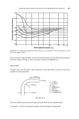


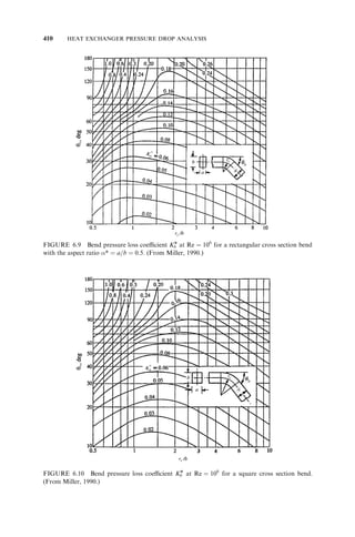
![288 ADDITIONAL CONSIDERATIONS FOR THERMAL DESIGN OF RECUPERATORS
re;i
¼ X‘
tanðiÞ tan½ði 1Þ
1=2
re; j
¼
X2
þ ðXt =2Þ2 1=2
‘
2
tanð j Þ tan½ð j 1Þ
1=2
ð4:154Þ
The fin efficiency of each sector is then determined by the circular fin of constant cross
section [Eq. (4.151)]. Once f for each sector is determined, f for the entire fin is the
surface-area weighted average of f ’s for each sector.
f
¼
Pmi
¼1 f ;i Af ;i
þ aPnj
¼1 f ; jAf ; j
Pmi
¼1 Af ;i
þ aPnj
¼1 Af ; j
ð4:155Þ
Here a ¼ 1 for inline arrangement (Fig. 4.16c) for segment OBC and n ¼ 2 for staggered
arrangement (Fig. 4.16d) for two equal segments, ODE and OEF. This approximation
improves as the number of sectors m, n!1. However, in reality, only a few sectors m
and n will suffice to provide f within the desired accuracy (such as 0.1%). An implicit
assumption made in this method is that the heat flow is only in the radial direction and
not in the path of least thermal resistance. Hence, f calculated by the sector method will
be lower than that for the actual flat fin, a conservative value. However, the equivalent
annulus method yields an f that may be considerably higher than that by the sector
method, particularly when the fin geometry around the circular tube departs more and
more from a square fin; as a result, the heat transfer computed will be too high.
4.3.3 Fin Effectiveness
Another measure of fin heat transfer performance is the fin effectiveness. It is a ratio of
actual heat transfer rate through the fin base area to the heat transfer rate through the
same fin base area ðAk;Þ 0
if the fin were removed. Thus,
¼ q0
hAk;00
ð4:156Þ
This concept is useful for the first three boundary conditions of Fig. 4.10, and particu-larly
for the most common boundary condition of an adiabatic fin tip. In the definition of
, it is idealized that the heat transfer coefficient at the fin base when the fin is removed is
identical to the heat transfer coefficient at the fin surface. Using the q0 expression of Eq.
(4.134) for the thin straight fin with an adiabatic fin tip, of Eq. (4.156) is related to f as
¼
Af
Ak;0
f
¼
þ
‘
Lf
2 Lf
f
2‘
f
ð4:157Þ
where it is idealized that Lf
for the term after the approximate equality sign. This
equation is also applicable to the fin of an infinite length. A similar relationship can also
be developed between and f using q0 of Eq. (4.131) for a fin with the convective
boundary at the fin tip.](https://image.slidesharecdn.com/fundamentalsofheatexchangerdesign-131001160835-phpapp01-141008073824-conversion-gate02/85/Fundamentalsofheatexchangerdesign-131001160835-phpapp01-442-320.jpg)
![ADDITIONAL CONSIDERATIONS FOR EXTENDED SURFACE EXCHANGERS 289
The following observations can be made from Eq. (4.157):
. The explicit formula for can be obtained when the expression for f is available.
Of course, Eq. (4.157) needs to be modified by substituting q0 from Eq. (4.131) in
Eq. (4.156) for a thin fin with convective boundary at the fin tip.
. will generally be much greater than unity. For a typical automotive radiator,
‘ 3mm and
0.075 mm. Hence,
75! In a good design, must exceed a
minimum of 2.
. All parameters that increase f [see the discussion in Section 4.3.2.1 after Eq.
(4.137)] will also increase except for ‘ and
. Note that an increase in ‘ will
increase m‘ and reduce f (see Fig. 4.14). However, the reduction in f is much
smaller than the increase in ‘ on a percentage basis. Since is directly proportional
to ‘, the overall will increase linearly with an increase in ‘. Similarly, as noted
above, an increase in
increases f, but at a much lower rate, while is inversely
proportional to
from Eq. (4.157). Hence, overall will increase with a decrease in
. Thus, will increase with an increase in ‘ and kf and a decrease in
and h.
4.3.4 Extended Surface Efficiency
An extended surface exchanger has fins attached to the primary surface by brazing,
soldering, welding, adhesive bonding, mechanical (press) fit, or extrusion, such as the
plate-fin exchanger section shown in Fig. 4.17a. In a plate-fin exchanger, fins are spaced
sufficiently far apart to allow desired fluid flow rate (that produces pressure drop within
allowed limits) and to have minimum fouling potential. The primary surface Ap is then
exposed between fins as shown in Fig. 4.17a. In most tube-fin designs, there is also a
primary surface exposed to the fluid along with the fins (secondary surface) as shown in
Fig. 4.17b. The heat transfer performance of this extended surface is measured by an
extended (or overall) surface efficiency o, defined as{
o
¼ qtotal
qmax
¼
qp
þ qf
h Ap
þ Af
ð T1Þ
T0
ð4:158Þ
In this equation the definition of qmax is similar to that defined by Eq. (4.130) for an
adiabatic fin tip with an added heat transfer component for the primary surface. We have
also redefined Af and qf
ð¼ q0
Þ as total values for all finned surfaces; we also redefine f
using the values of Af and qf for all finned surfaces instead of a single fin. Also, Ap in Eq.
(4.158) represents the total primary surface area associated with the particular fluid side
of concern in the exchanger. We have idealized heat transfer coefficients for the primary
and fin surface areas as the same in Eq. (4.158). Now the total heat transfer rate qtotal is
given by
qtotal
¼ qp
þ qf
¼ hAp T0
T1 ð Þþ hAf f T0
T1 ð Þ¼ hðAp
þ fAf
Þ T0
T1 ð Þ
ð4:159Þ
Substituting Eq. (4.159) into Eq. (4.158), and simplifying yields
o
¼ 1
Af
A
ð4:160Þ
1 f
{ For the case of finite heat transfer at the fin tip with he as the actual or equivalent heat transfer coefficient, replace
Af with Af
þ ðh=he
ÞAk in Eqs. (4.158), (4.160), (4.162), and (4.163), and Af with ðAf
þ Ak
Þ in Eq. (4.158).](https://image.slidesharecdn.com/fundamentalsofheatexchangerdesign-131001160835-phpapp01-141008073824-conversion-gate02/85/Fundamentalsofheatexchangerdesign-131001160835-phpapp01-443-320.jpg)


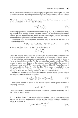
![HEAT TRANSFER ANALYSIS 315
Combining it with Eq. (5.7) and simplifying, we get
@Tw;h
@h
¼ ðhAÞ
h
Cr;hPh
ðTh
Tw;h
Þ ð5:17Þ
Cold Period: Fluid and Matrix. For the cold-gas flow period, a pair of equations similar
to Eqs. (5.14) and (5.17) results:
@Tc
@c
þ L
d;c
@Tc
@x
¼ hA ð Þ
c
Ccd;c
ð5:18Þ
Tc
Tw;c
@Tw
@c
¼ hA ð Þ
c
Cr;cPc
Tw;c
Tc
ð5:19Þ
The boundary conditions are as follows. The inlet temperature of the hot gas is constant
during the hot-gas flow period, and the inlet temperature of the cold gas is constant
during the cold-gas flow period:
ð Þ¼T
Th 0; h
h;i
¼ constant for 0 h
Ph
ð5:20Þ
ð Þ¼T
Tc L; c
c;i
¼ constant for 0 c
Pc
ð5:21Þ
The periodic equilibrium conditions for the wall are
ð Þ¼ Tw;c x; c
Tw;h x; h
¼ Ph
ð ¼ 0Þ for 0 x L ð5:22Þ
ð ¼ 0Þ ¼ Tw;c x; c
Tw;h x; h
ð Þ for 0 x L ð5:23Þ
¼ Pc
Since the regenerator is in periodic equilibrium, Eqs. (5.20)–(5.23) are valid for
¼ þ nPt, where n is an integer, n 0.
The boundary conditions of Eqs. (5.20) and (5.21) are simplest for the analysis. The
corresponding analytical models can be solved using analytical and seminumerical
methods. In applications, the hot- and cold-fluid inlets to the regenerator may have
nonuniform temperature profiles. Then the solution can only be obtained by a numerical
analysis.
Based on the foregoing differential equations and boundary conditions [Eqs. (5.14)
and (5.17)–(5.23)], the dependent fluid and matrix temperatures are functions of the
following variables and parameters:
Th;Tc;Tw
|fflfflfflfflfflffl{zfflfflfflfflfflffl}
dependent
variables
¼ ½x; h; c
; Th;i ; Tc;i ; Ch; Cc; d;h; d;c;
|fflfflfflffl{zfflfflfflffl}
independent
variables
|fflfflfflfflfflfflfflfflfflfflfflfflfflfflfflfflfflfflfflfflfflfflffl{zfflfflfflfflfflfflfflfflfflfflfflfflfflfflfflfflfflfflfflfflfflfflffl}
operating condition
variables
Cr; ðhAÞ
h; hA ð Þ
c; L; Ph; Pc
|fflfflfflfflfflfflfflfflfflfflfflfflfflfflfflfflfflfflfflfflfflfflfflfflffl{zfflfflfflfflfflfflfflfflfflfflfflfflfflfflfflfflfflfflfflfflfflfflfflfflffl}
parameters under designer’s control
ð5:24Þ
Neither Cr;c nor Cr;h is included in the foregoing list since Cr;c
¼ Cr;h
¼ Cr [see Eq. (5.8)].
The regenerator fluid and wall temperatures are thus dependent on 14 independent
variables and parameters (since is the independent time variable designated with the
subscripts h and c for ease of understanding) . Through nondimensionalization we obtain](https://image.slidesharecdn.com/fundamentalsofheatexchangerdesign-131001160835-phpapp01-141008073824-conversion-gate02/85/Fundamentalsofheatexchangerdesign-131001160835-phpapp01-479-320.jpg)


![matrix, the fluid outlet temperatures are functions of the time . In this case, the time-averaged
outlet temperatures are
Th;o
¼ 1
Ph
ðPh
0
Th;oðÞ d; Tc;o
¼ 1
Pc
ðPc
0
Tc;oðÞ d ð5:41Þ
Here Th;o
ðÞ and Tc;o
ðÞ are the time-dependent fluid temperatures at the regenerator
outlet. Th;o and Tc;o in Eqs. (5.40) and (5.41), respectively, represent the space- and time-averaged
fluid temperatures at the regenerator outlet. Equation (5.41) is valid for both
the fixed-matrix and rotary regenerators, provided that an observer rides on the matrix
for a rotary regenerator.
Thus, the functional relationship of Eq. (5.39) for the dependent regenerator average
outlet temperatures is
T*h
;o; T*c
;o
¼ ðntuh; ntuc; C*r
;h; C*r
;c
Þ ð5:42Þ
A bar on these dimensionless as well as dimensional [of Eq. (5.41)] average outlet tem-peratures
is eliminated for convenience (like in a recuperator) in the rest of the chapter,
except where such terminology could create ambiguity.
These outlet temperatures are conveniently expressed by the regenerator effectiveness
¼ q=qmax. Using the outlet temperatures defined by Eq. (5.41), the actual heat transfer
rate in the rotary regenerator is
q ¼ Ch
ðTh;i
Th;o
Þ ¼ Cc
ð Tc;o
Tc;i
Þ ð5:43Þ
In this section we have considered either a rotary regenerator or all matrices of a fixed-matrix
regenerator as a system. The hot and cold fluids flow continuously in and out of
such a system. To determine qmax for such a system, we define a ‘‘perfect’’ heat exchanger
as defined for recuperators after Eq. (3.37). This perfect heat exchanger is a counterflow
recuperator of infinite surface area, zero longitudinal wall heat conduction, and zero flow
leakages from one fluid to another fluid, operating with fluid flow rates and fluid inlet
temperatures the same as those of an actual regenerator; fluid properties are considered
constant for both exchangers. qmax for this perfect heat exchanger as in Eq. (3.42) is
qmax
ð5:44Þ
¼ Cmin Th;i
Tc;i
where Cmin is the minimum of Ch and Cc. The regenerator effectiveness is thus
¼ q
qmax
¼
Ch Th;i
Th;o
Cmin Th;i
Tc;i
¼
Cc Tc;o
Tc;i
Cmin Th;i
Tc;i
ð5:45Þ
Then for Cc
¼ Cmin, comparing with T*h
;o
¼ 1 C* and T*c
;o
¼ from the definitions
in Eq. (5.28) for the outlet temperatures, we get
¼ 1 T*h
;o
C*
¼ T*c
;o
ð5:46Þ
and Eq. (5.42) in terms of is
¼ ðntuh; ntuc; C*r
;h; C*r
;c
Þ ð5:47Þ
318 THERMAL DESIGN THEORY FOR REGENERATORS](https://image.slidesharecdn.com/fundamentalsofheatexchangerdesign-131001160835-phpapp01-141008073824-conversion-gate02/85/Fundamentalsofheatexchangerdesign-131001160835-phpapp01-482-320.jpg)
![THE -NTUo METHOD 319
Since these independent dimensionless groups, defined in Eqs. (5.29) and (5.30), are
not parallel to those of a recuperator (a direct-transfer exchanger), let us define a related
set as follows:
NTUo
¼ 1
Cmin
1
1=ðhAÞ
h
þ 1=ðhAÞ
c
ð5:48Þ
C* ¼ Cmin
Cmax
ð5:49Þ
Cr *
¼ Cr
Cmin
ð5:50Þ
ðhAÞ* ¼
ðhAÞ on the Cmin side
ðhAÞ on the Cmax side
ð5:51Þ
Since Eqs. (5.48)–(5.51) utilize only four independent dimensionless groups [to be shown
related to those of Eq. (5.47)], it is then valid to recast Eq. (5.47) as
¼ ½NTUo;C*; Cr *
; ðhAÞ* ð5:52Þ
Here NTUo is the modified number of transfer units. Since there is no direct heat transfer
from the hot fluid to the cold fluid in a regenerator (similar to that in a recuperator), UA
does not come into the picture directly for the regenerator. However, if the bracketed
term of Eq. (5.48) is designated as UoA, with Uo termed as a modified overall heat transfer
coefficient, then
1
UoA
¼ 1
ðhAÞ
h
þ 1
ðhAÞ
c
and NTUo
¼ UoA
Cmin
ð5:53Þ
A comparison of this expression with Eq. (3.24) or (3.20) reveals that UoA is the same as
UA when the wall thermal resistance and fouling resistances are zero. Note that the entire
surface in a regenerator is primary surface (no fins), and hence the overall extended
surface efficiency ¼ o
1. Thus the definition of NTUo
¼ UoA=Cmin parallels that of
NTU of Eq. (3.59), and in the limiting case of Cr *
¼1, the numerical solutions demon-strate
that the regenerator has the same performance as a recuperator with its NTUo
identical to NTU provided that the pressure and carryover leakage effects are neglected.
The newly defined dimensionless groups of Eq. (5.52) are related to those of Eq. (5.47) as
follows for Cc
¼ Cmin:
NTUo
¼ 1
ðC*r
;h=C*r
;c
Þ=ntuh
þ 1=ntuc
ð5:54Þ
C* ¼ C*r
;h
C*r
;c
ð5:55Þ
Cr *
¼ C*r
;c
ð5:56Þ
ðhAÞ* ¼ ntuc
ntuh
C*r
;h
C*r
;c
ð5:57Þ](https://image.slidesharecdn.com/fundamentalsofheatexchangerdesign-131001160835-phpapp01-141008073824-conversion-gate02/85/Fundamentalsofheatexchangerdesign-131001160835-phpapp01-483-320.jpg)

![THE -NTUo METHOD 321
on the regenerator effectiveness for the range 0:25 ðhAÞ* 4. Since most regenerators
operate in this range of ðhAÞ*, fortunately, the effect of ðhAÞ* on the regenerator effec-tiveness
can usually be ignored.
r 5.2.4 e-*
NTUo Results for a Counterflow Regenerator
No closed-form exact solution of the theoretical model [Eqs. (5.31)–(5.38)] is available
presently. The solutions mentioned below are obtained to determine the regenerator
effectiveness directly, and not the detailed temperature distributions. A numerical
solution to Eqs. (5.31)–(5.38) has been obtained by Lamberston (1958) using a finite
difference method and a closed-form approximate solution by Bacˇ lic´ (1985) using a
Galerkin method. Lamberston (1958) employed a finite difference method to analyze a
rotary regenerator. He presented the solution in terms of as a function of the four
dimensionless groups of Eq. (5.52). He covered the following range of the parameters:
1 NTUo
10, 0:1 C* 1:0, 1 C1, and 0:25 ðhAÞ* 1. His results are
r presented by *
Kays and London (1998). A closed-form solution for a balanced
(C* ¼ 1) and symmetric ½ðhAÞ* ¼ 1 counterflow regenerator has been obtained by
Bacˇ lic´ (1985), valid for all values of C 1 as follows:
¼ Cr *
1 þ 72
24 B 2 R1
f ½ ð þ 2EÞg
A1
90 N1
1 þ 92
24fB 6½R A 20ðN 3EÞg
ð5:58Þ
100
90
80
70
60
50
0 2 4 6 8 10
NTUo
ε%
1.0
1.5
2.0
5.0
C*r
= ∞
0.25 ≤ (hA)* ≤ 4
FIGURE 5.3 Counterflow regenerator as a function of NTUo and for C* ¼ 1 (Kays and
London, 1998).](https://image.slidesharecdn.com/fundamentalsofheatexchangerdesign-131001160835-phpapp01-141008073824-conversion-gate02/85/Fundamentalsofheatexchangerdesign-131001160835-phpapp01-485-320.jpg)


![338 THERMAL DESIGN THEORY FOR REGENERATORS
If the temperatures Th, Tc, and Tw are made dimensionless as before [Eq. (5.28)], it is
evident from Eqs. (5.69)–(5.72) that
Th*;Tc*; Tw* ¼ ð h; c; h; c
Þ ð5:74Þ
For overall regenerator performance, we are interested in determining the time-aver-aged
fluid outlet temperatures. These temperatures are obtained from their definitions
[Eq. (5.41)] after suitable modifications based on Eq. (5.69), with replaced by h and c
for the hot- and cold-gas flow periods, respectively. These temperatures are expressed by
the regenerator effectiveness. Since we have considered only one matrix at a time in the
foregoing analysis, the hot and cold fluid flows are intermittent. In an ideal steady-state
periodic condition, the actual heat transfer ( joules or Btu) during one hot- or cold-gas
flow period will be
Q ¼ ChPh Th;i
Th;o
¼ CcPc Tc;o
Tc;i
ð5:75Þ
This means that the regenerator is in a cyclic equilibrium because the heat transferred to
the matrix during the hot period equals the heat transferred to the cold fluid during the
cold period. The maximum possible heat transfer will be in a counterflow regenerator of
infinite surface area having the same fluid flow rates and fluid inlet temperatures. Thus
this maximum possible heat transfer is
Qmax
¼ ðCPÞ
min
ðTh;i
Tc;i
Þ ð5:76Þ
Thus, the effectiveness for a fixed-matrix regenerator (with two matrices) is defined as
follows:
¼ Q
Qmax
¼
ðCPÞ
h
ðTh;i
Th;o
Þ
min
ðTh:i
ðCPÞ
Tc;i
Þ
¼
ðCPÞ
c
ð Tc;o
Tc;i
Þ
ðCPÞ
min
ðTh:i
Tc;i
Þ
ð5:77Þ
However, the effectiveness of a single matrix of two or more matrices of a fixed-matrix
regenerator can be defined as follows by considering only one matrix going through the
hot and cold period (i.e., one complete period). The maximum possible heat transfer
during hot- and cold-gas flow periods, respectively, is
Qmax;h
¼ ChPh Th;i
Tc;i
Qmax;c
¼ CcPc Th;i
Tc;i
ð5:78Þ
Thus, the regenerator effectiveness during hot- and cold-gas flow periods are
h
¼ Qh
Qmax;h
¼ ChPh
ðTh;i
Th;o
Þ
ChPh
ðTh;i
Tc;i
Þ
¼ Th;i
Th;o
Th;i
Tc;i
¼ 1 T*h
;o
ð5:79Þ
c
¼ Qc
Qmax;c
¼ CcPc
ð Tc;o
Tc;i
Þ
CcPc
ðTh;i
Tc;i
Þ
¼
Tc;o
Tc;i
Th;i
Tc;i
¼ T*c
;o
ð5:80Þ
where the last equalities in Eqs. (5.79) and (5.80) are obtained using the definitions of Eq.
(5.28). Note that the effectiveness in Eqs. (5.79) and (5.80) is similar to the temperature
effectiveness for a recuperator [Eqs. (3.51) and (3.52)]. Razelos (1979) defined the overall](https://image.slidesharecdn.com/fundamentalsofheatexchangerdesign-131001160835-phpapp01-141008073824-conversion-gate02/85/Fundamentalsofheatexchangerdesign-131001160835-phpapp01-502-320.jpg)
![effectiveness of a single matrix as
r
¼ Qh
þ Qc
Qmax;h
þ Qmax;c
THE - METHOD 339
¼ 2Q
Qmax;h
þ Qmax;c
ð5:81Þ
Using Eqs. (5.79)–(5.81), it can be shown that
1
r
¼ 1
2
1
h
þ 1
c
therefore, r
¼ 2ðCc=Ch
Þ
1 þ ðCc=Ch
Þ c
ð5:82Þ
Comparing Eqs. (5.77) and (5.82), it can be shown for a two-matrix regenerator that
¼ 1 þ C*
2C*
r
ð5:83Þ
The independent dimensionless variables of Eqs. (5.69), collocated at x ¼ L, h
¼ Ph
or c
¼ Pc, become the dimensionless parameters as follows{:
j
¼ j
ðLÞ ¼ hA
C
j
j
¼ hA
¼ j Pj
Cr
j
Pj j ¼ h or c ð5:84Þ
Hence, the regenerator effectiveness is a function of four parameters:
¼ ðh; c;h;c
Þ ð5:86Þ
From the first equation of Eq. (5.84), j
¼ j
ðLÞ; and from Eq. (5.73), ðLÞ ¼ bL, we get
¼ bL ð5:87Þ
Similarly, from the second equation of Eq. (5.84), j
¼ j
ðPj
Þ; and from Eq. (5.73),
j
ðPj
Þ ¼ cPj . Hence, we get
¼ cPh or cPc
ð5:88Þ
Since b and c are constants in Eqs. (5.87) and (5.88), and are designated as reduced
length and reduced period, respectively, for the regenerator. The reduced length also
designates the dimensionless heat transfer or thermal size of the regenerator [see, e.g., Eq.
(5.107)], and this method is referred to as the - method. It has been used primarily for
the design of fixed-matrix regenerators, but of course it can also be used for the design of
rotary regenerators. In the - method, several different designations are used to classify
regenerators, depending on the values of and . Such designations and their equivalent
dimensionless groups of the -NTUo method are summarized in Table 5.2.
For the effectiveness of the most general unbalanced and unsymmetrical regenerator,
Razelos (1979) proposed an alternative set of four dimensionless groups, instead of those
of Eq. (5.86):
; r; h; c
¼ m;m ð ;
;R*Þ ð5:89Þ
{ If the dwell periods d;h and c;h are not negligible, h and c would be
h
¼ h
ðPh
Þ ¼ hhAh
Cr;h
ðPh
d;h
Þ c
¼ c
ðPc
Þ ¼ hcAc
Cr;c
ðPc
d;c
Þ ð5:85Þ](https://image.slidesharecdn.com/fundamentalsofheatexchangerdesign-131001160835-phpapp01-141008073824-conversion-gate02/85/Fundamentalsofheatexchangerdesign-131001160835-phpapp01-503-320.jpg)


![INFLUENCE OF LONGITUDINAL WALL HEAT CONDUCTION 349
Using the previous definitions of X*, h*, Th*, Tw*, ntuh, and C*r
;h [Eqs. (5.25)–(5.30)],
Eq. (5.110) is made dimensionless:
@Tw*
@h*
¼ ntuh
C*r
;h
Th* Tw ð *Þ þ h
C*r
;h
@2Tw*
@X*2
ð5:111Þ
where
h
¼ kwAk;h
LCh
ð5:112Þ
Similarly, the governing differential equation for the matrix wall temperature during the
cold-gas flow period is
@Tw*
@c*
¼ ntuc
C*r
;c
Tw* Tcð *Þ þ c
C*r
;c
@2Tw*
@X*2
ð5:113Þ
where
c
¼ kwAk;c
LCc
ð5:114Þ
Since Eqs. (5.111) and (5.113) are second-order partial differential equations with
respect to X*, we need to define four boundary conditions for the matrix wall tempera-tures
in order to get a particular solution: two during the hot-gas flow period and two
during the cold-gas flow period. The realistic boundary conditions are adiabatic bound-ary
conditions for each period at X* ¼ 0 and 1:
@Tw*
@X*
X¼0
¼
@Tw*
@X*
X¼1
¼ 0 for 0 h* 1
@Tw*
@X
X¼1
¼ 0 for 0 c* 1
8
:
ð5:115Þ
ð5:116Þ
Thus, the inclusion of the effect of longitudinal heat conduction adds two dimensionless
groups, h and c, on which the exchanger effectiveness would depend. Bahnke and
Howard (1964) suggested an alternative set of two dimensionless groups:
¼ kwAk;t
LCmin
Ak* ¼ Ak on the Cmin side
Ak on the Cmax side
ð5:117Þ
where Ak;t is the total area for longitudinal conduction,
Ak;t
¼ Ak;h
þ Ak;c
¼ Afr
Ao
¼ Afr
ð1 Þ ð5:118Þ
Note that and Ak* are related to h and c as follows for Cc
¼ Cmin:
¼ c
þ h
C*
Ak* ¼ Ak;c
Ak;h
¼ C*
c
h
ð5:119Þ](https://image.slidesharecdn.com/fundamentalsofheatexchangerdesign-131001160835-phpapp01-141008073824-conversion-gate02/85/Fundamentalsofheatexchangerdesign-131001160835-phpapp01-513-320.jpg)


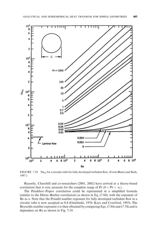


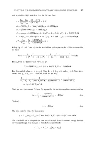
![in the regenerator are linear with time, and the numerical value of this time derivative of
temperature at any point in the wall is the same. For the wall temperature, this means
@Tw
@
¼ @Tw;o
@
¼ @Tw;m
@
¼ constant ð5:125Þ
Here Tw;o and Tw;m are the surface wall temperature and mean wall temperature at a
given instant in time. This linear temperature–time relationship represents a good
approximation to the actual wall temperature profile in the greater part of either hot-or
cold-gas flow period along most of the regenerator length, as shown in Fig. 5.9.
Now let us consider a differential element of the regenerator matrix wall as shown
in Fig. 5.12 during the hot-gas flow period. Here Aw represents the conduction area for
the wall for heat conduction in the y direction. For continuous flow passages, Aw
¼ A
(the convective heat transfer surface area), and Aw
A for noncontinuous flow passages.
The energy balance on the element of Fig. 5.12b yields the well-known one-dimensional
transient conduction equation valid at each x coordinate.
w
@2Tw
@y2
¼ @Tw
@
ð5:126Þ
where w
¼ kw=wcw is the thermal diffusivity of the matrix material. The appropriate
boundary conditions are (see Fig. 5.12)
Tw
¼ Tw;o at y ¼ 0 and
w
ð5:127Þ
356 THERMAL DESIGN THEORY FOR REGENERATORS
dy
Th,m Th,m
–
∂Tw ∂Tw
∂y ∂τ (ρwAwdycw) ––– ∂Tw ∂2Tw
dy
dy
dQ dA dx
x x
Tw
Tw
δw δw
Tw,o
Tw,o
Tw,o
Tw,m
Tw,o
y
(a)
(b)
(c)
Section x
– kw Aw –––– – kw Aw
∂y ∂y2 [–––– + ––––]
–
–
–
FIGURE 5.12 (a) Matrix wall of thickness
w, (b) energy transfer terms across the differential wall
element; (c) parabolic temperature distribution in the wall at a given x (From Shah, 1981).](https://image.slidesharecdn.com/fundamentalsofheatexchangerdesign-131001160835-phpapp01-141008073824-conversion-gate02/85/Fundamentalsofheatexchangerdesign-131001160835-phpapp01-521-320.jpg)


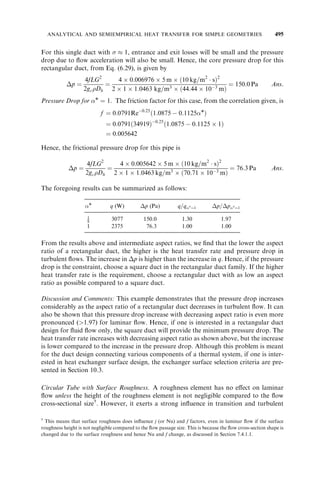


![364 THERMAL DESIGN THEORY FOR REGENERATORS
Generally, the carryover leakage is very small and its influence on the regenerator effec-tiveness
is also negligibly small for most rotary regenerator applications, except for the
cryogenics and Stirling engine regenerators, which have effectively a very high value of
switching frequency.
The leakage modeling of an actual regenerator involves the determination of all nine
leakage flow rates mentioned in Table 5.6, plus mass flow rates, pressures, and tempera-tures
at the mixing points A, B, . . . , F in Fig. 5.14. To be more specific, four additional
mass flow rate terms are hot- and cold-gas mass flow rates through the regenerator disk
ðm_ h;m_ c
Þ, and hot- and cold-gas mass flow rates at the outlet of the actual regenerator
ðm_ h;o;m_ c;o
Þ; four pressures and temperatures at points B and E of Fig. 5.14: ph*, pc*, Th*,
Tc* (note these are dimensional values); and three temperatures from the actual regen-erator
0
h;i . Thus it represents a
to the outside or to an internal regenerator: Th;o, Tc;o, and T
total of 20 unknowns for the actual regenerator. Determination of various leakage flow
rates of Table 5.6 represents nine equations [seven of Eq. (5.149) and two of Eq. (5.150)].
The mass flow rate balances at six junction points A, B, . . . , F in Fig. 5.14 represent six
equations presented in Table 5.7. The energy balances at five points, A, B, C, E, and F in
Fig. 5.14, provide an additional five equations, as summarized in Table 5.8. Thus a total
of 20 linear/nonlinear equations are available to determine 20 unknowns mentioned
above. If m_
ðCÞ
c;r leaks from point C to D in Fig. 5.14, one additional energy balance
0
c;i .
equation at point D is available in Table 5.8, and the additional unknown is T
To investigate the influence of leakage distribution on regenerator heat transfer per-formance,
we also need to consider heat transfer and pressure drop modeling of the
internal regenerator. Heat transfer analysis includes applying -NTUo theory, including
longitudinal and transverse wall heat conduction effects, discussed in Sections 5.2, 5.4,
and 5.5 for the internal regenerator. Here the appropriate mass flow rates and inlet
temperatures are determined for the internal regenerator from an analysis of the actual
regenerator as mentioned above. The internal regenerator heat transfer analysis will then
yield temperatures and the internal regenerator effectiveness i;b. The pressure drop
analysis for the hot- and cold-gas sides of the internal regenerator is also straightforward
and is presented in Chapter 6. Appropriate flow rates within the internal regenerator and
TABLE 5.7 Mass Flow Rate Balances at Mixing Locations in the Regenerator
Mixing Location Pressure Condition Mass Flow Rate Balance
A ph;i ph* m_ h;i
m_
ðHÞ
c;r
þ m_
ðHÞ
h; p
þ m_ h;co
þ m_ h
¼ 0
ph;i ph* m_ h;i
m_
ðHÞ
c;r
m_
ðHÞ
h; p
þ m_ h;co
þ m_ h
¼ 0
B ph;i ph* m_
ðHÞ
h; p
m_ c;ax
þ m_
ðCÞ
h; p
¼ 0
ph;i ph* m_
ðHÞ
h; p
m_ c;ax
þ m_
ðCÞ
h; p
¼ 0
C m_ h
m_
ðCÞ
c;r
m_
ðCÞ
h; p
m_ c;co
þ m_ h;o
¼ 0
D m_ c;i
þ m_ c;co
þ m_
ðCÞ
c; p
þ m_
ðCÞ
c;r
þ m_ c
¼ 0
E pc;o pc *
m_
ðCÞ
c; p
m_
ðHÞ
c; p
þ m_ c;ax
¼ 0
pc;o pc *
m_
ðCÞ
c; p
þ m_
ðHÞ
c; p
þ m_ c;ax
¼ 0
F pc;o pc *
m_ c
m_ h;co
þ m_
ðHÞ
c; p
þ m_
ðHÞ
c;r
þ m_ c;o
¼ 0
pc;o pc *
m_ c
m_ h;co
m_
ðHÞ
c; p
þ m_
ðHÞ
c;r
þ m_ c;o
¼ 0
Source: Data from Shah and Skiepko (1997).](https://image.slidesharecdn.com/fundamentalsofheatexchangerdesign-131001160835-phpapp01-141008073824-conversion-gate02/85/Fundamentalsofheatexchangerdesign-131001160835-phpapp01-529-320.jpg)


![SUMMARY 371
From the foregoing values, we can compute NTUo, given in Eq. (5.48), as
NTUo
¼ 1
Cmin
1
1=ðhAÞ
h
þ1=ðhAÞ
c
¼ 1
43:25kW=K
1
ð1=440:9 þ 1=330:0ÞK=kW
¼ 4:364
Now determine the regenerator using Eqs. (5.62) and (5.63):
cf
¼ 1 exp NTUo 1 C* ½ ð Þ
1 C* exp½NTUoð1 C*Þ
¼ 1 exp 4:364 1 0:7625 ½ ð Þ
1 0:7625 exp½4:364ð1 0:7625Þ
¼ 0:8845
¼ cf 1 1
1:93
9Cr *
!
¼ 0:8845 1 1
9 15:221:93
¼ 0:8840
It can be shown that calculated by the Razelos method [Eqs. (5.64)–(5.67)] would have
been identical to 0.8840. The heat transfer rate is then determined as
¼ 0:8840 43:25kW=Kð339 29Þ8C ¼ 11,852 kW Ans:
q ¼ Cmin Th;i
Tc;i
Knowing the heat transfer rate, the hot- and cold-fluid outlet temperatures are cal-culated
as
Th;o
¼ Th;i
q
Ch
¼ 3398C 11,852kW
56:72kW=K
¼ 130:08C Ans:
Tc;o
¼ Tc;i
þ q
Cc
¼ 298C þ 11,852kW
43:25kW=K
¼ 303:08C Ans:
Discussion and Comments: This example illustrates the methodology of analyzing a
regenerator with multilayer packing. As discussed in the text, the multilayer packing is
used to accommodate high temperatures, high fouling and corrosion, and/or high matrix
volumetric heat capacity rates in different regions of the regenerator. The analysis above
presumes that the fluid temperature distribution is uniform after leaving the first zone
and entering the second zone on each fluid side. This is a reasonably good approxima-tion,
considering the fact that there are large uncertainties involved in the determination
of heat transfer coefficients and various flow leakages associated with regenerator
analysis. Once the problem is reformulated having an equivalent single layer, the analysis
is straightforward, as outlined in Section 5.2 since we have neglected the longitudinal wall
conduction effect.
SUMMARY
r *
Regenerators differ from recuperators in that the heat is transferred intermittently from
the hot fluid to the cold fluid via periodic thermal energy storage and release from the
heat transfer surface (matrix). As a result, two additional parameters enter in the analysis
of regenerators: the storage heat capacity rate of the matrix wall and the ratios of the
thermal conductances between the wall and hot and cold fluids [in a dimensionless form
Cand (hA)*, respectively], with the latter group of less importance in most industrial
regenerators. The two most commonly used methods for the design and analysis of](https://image.slidesharecdn.com/fundamentalsofheatexchangerdesign-131001160835-phpapp01-141008073824-conversion-gate02/85/Fundamentalsofheatexchangerdesign-131001160835-phpapp01-536-320.jpg)


![INTRODUCTION 379
by the saturation temperature change for a condensing/evaporating fluid if there is a
large pressure drop associated with the flow. This is because saturation temperature
changes with changes in saturation pressure and in turn affects the temperature potential
for heat transfer.
Let us first determine the relative importance of the fluid pumping power P for gas
flow vs. liquid flow in a heat exchanger. P is proportional to p in a heat exchanger and
is given by
P ¼
_V
V p
p
¼ m_ p
p
ð6:1Þ
where _V
V is the volumetric flow rate and p is the pump/fan efficiency. Now introduce the
following relationships:
m_ ¼ GAo p f
4L
Dh
G2
2gc
Re ¼ GDh
ð6:2Þ
where G is referred to as the core mass velocity ðG ¼ um
Þ, Ao is the minimum free flow
area, f is the Fanning friction factor,
y
and Re is the Reynolds number as defined in Eq.
(6.2). The p expression in Eq. (6.2) is for the core frictional pressure drop and is derived
later as Eq. (6.29). Substituting the expressions of Eq. (6.2) into Eq. (6.1) and simplifying
results in
P ¼ m_ p
p
1
2gcp
2
4L
Dh
m_ 2
DhAo
ð f ReÞ for fully developed laminar flow ð6:3aÞ
0:046
2gcp
0:2
2
4L
Dh
m_ 2:8
A1:8
o D0:2
h
for fully developed turbulent flow ð6:3bÞ
8
:
0:2 [see Eq. (7.72) in Table 7.6] is used in the derivation of the right-hand-
Here f ¼ 0:046Re
side expression of Eq. (6.3b) for fully developed turbulent flow.
z
Note also that
f Re in Eq. (6.3a) is constant for fully developed laminar flow, as discussed in Section
7.4.1.1. To determine the order of magnitude for the fluid pumping power requirement
for gas vs. liquid flow, let us assume that the flow rate and flow passage geometry are
given (i.e., m_ , L, Dh, and Ao are specified). It is evident from Eq. (6.3) that P / 1=2 (i.e.,
strongly dependent on in laminar and turbulent flows);P / (i.e., strongly dependent
on in laminar flow); and P / 0:2 (i.e., weakly dependent on in turbulent flow). For
high-density moderate-viscosity liquids, the pumping power is generally so small that it
has only a minor influence on the design. For laminar flow of highly viscous liquids in
large L=Dh exchangers, the fluid pumping power is an important constraint. In addition,
the pumping power is an important consideration for gases, in both turbulent and
laminar flow, because of the great impact of 1/2. For example, the density ratio for
liquid water vs. air at ambient conditions is approximately 800 : 1, which indicates that
the pumping power for airflow will be much higher than that for water if p is to be kept
y
The definition of the Fanning friction factor is given in Eq. (6.9).
z
It should be emphasized that Eqs. (6.3a) and (6.3b) are presented for demonstrating the importance of p, and
they do not imply that we avoid the transition flow regime. As a matter of fact, most automotive heat exchangers
operate in the transition regime. We discuss the range of Re for laminar, transition, and turbulent flows in heat
exchangers in Section 7.1.2.2.](https://image.slidesharecdn.com/fundamentalsofheatexchangerdesign-131001160835-phpapp01-141008073824-conversion-gate02/85/Fundamentalsofheatexchangerdesign-131001160835-phpapp01-544-320.jpg)
![380 HEAT EXCHANGER PRESSURE DROP ANALYSIS
the same. Hence, typical design values of p for water and air as working fluids in a heat
exchanger are 70 kPa (10 psi) (a typical value in shell-and-tube exchangers) and 0.25 kPa
(1 in. H2O) (for compact exchangers with airflows near ambient pressures), respectively,
to maintain the low fluid pumping power requirement for exchanger operation. Refer
also to the first footnote in Section 13.1 and the associated discussion.
6.1.2 Fluid Pumping Devices
The most common fluid pumping devices are fans, pumps, and compressors. A fan is a
low-pressure air- or gas-moving device, which uses rotary motion. There are two major
types of fans: axial and radial (centrifugal), depending on the direction of flow through
the device. Fans may be categorized as blowers and exhausters. A blower is a centrifugal
fan when it is used to force air through a system under positive pressure, and it develops a
reasonably high static pressure (500 Pa or 2.0 in.H2O). An exhauster is a fan placed at the
end of a system where most of the pressure drop is on the suction side of the fan. A pump
is a device used to move or compress liquids. A compressor is a high-volume centrifugal
device capable of compressing gases [100 to 1500 kPa (15 to 220 psi) and higher].
Fans and pumps are volumetric devices and are commonly used to pump fluids
through heat exchangers. This means that a fan will develop the same dynamic head
[pressure rise per unit fluid (gas) weight across the fan; Eq. (6.4)] at a given capacity
(volumetric flow rate) regardless of the fluids handled, with all other conditions being
equal. This means that the pressure rise across a fan will be proportional to the fluid
density at a given volumetric flow rate for all other conditions being equal. Note that the
head, dynamic head or velocity head is referred to as the kinetic energy per unit weight of
the fluid pumped, expressed in units of millimeters or inches (feet). Thus the pressure rise
across a fan (which is mainly consumed as the pressure drop across a heat exchanger) can
be expressed in terms of the head H as follows:
p
g=gc
¼ H ¼ u2
m
2g
ð6:4Þ
Since fans and pumps are generally head limited, the pressure drop in the heat exchanger
can be a major consideration.
6.1.3 Major Contributions to the Heat Exchanger Pressure Drop
The pressure drop associated with a heat exchanger is considered as a sum of two major
contributions: pressure drop associated with the core or matrix, and pressure drop
associated with fluid distribution devices such as inlet/outlet headers, manifolds, tanks,
nozzles, ducting, and so on. The purpose of the heat exchanger is to transfer thermal
energy from one fluid to the other; and for this purpose, it requires pressure difference
(and fluid pumping power) to force the fluid flow over the heat transfer surface in the
exchanger. Hence, ideally most of the pressure drop available should be utilized in
the core and a small fraction in the manifolds, headers, or other flow distribution devices.
However, this ideal situation may not be the case in plate heat exchangers and other heat
exchangers in which the pressure drop associated with manifolds, headers, nozzles, and
so on, may not be a small fraction of the total available pressure drop.
If the manifold and header pressure drops are small, the core pressure drop domi-nates.
This results in a relatively uniform flow distribution through the core. All heat](https://image.slidesharecdn.com/fundamentalsofheatexchangerdesign-131001160835-phpapp01-141008073824-conversion-gate02/85/Fundamentalsofheatexchangerdesign-131001160835-phpapp01-545-320.jpg)


![384 HEAT EXCHANGER PRESSURE DROP ANALYSIS
As discussed in Section 7.2.1.2, w represents the effective wall shear stress, and is the
fluid mass density determined at the local bulk temperature and mean pressure. Also
define the hydraulic radius rh as
rh
¼ Ao
P
ð6:10Þ
Note that the hydraulic diameter Dh
¼ 4rh; it was defined earlier by Eq. (3.65) and in the
footnote in Section 1.4.
Substituting Eqs. (6.9) and (6.10) into Eq. (6.8) and using dð1=Þ ¼ ð1=2Þ d, we
get, upon simplification,
dp
dx
¼ G2
2gc
2
2
d
dx
þ f
1
rh
ð6:11Þ
Integration of this equation from x ¼ 0 ð ¼ , p ¼ p2; see Fig. 4.1) to x ¼ L ði ¼ o,
p ¼ p3) will provide the expression for the core pressure drop p2¼ 3
p2
p3 as
p23
¼ G2
2gci
2
i
o
1
þ f
L
rh
i
1
m
ð6:12Þ
where the mean specific volume with respect to the flow length, (1=Þ
m, is defined as
1
m
¼ 1
L
ðL
0
dx
ð6:13Þ
Here, the fluid mean specific volume ð1=Þ
m can be expressed as follows [see also Eq.
(9.18)]. For a liquid with any flow arrangement, or for an ideal gas with C* ¼ 1 and any
flow arrangement except for parallelflow,
1
m
¼ vm
¼ vi
þ vo
2
¼ 1
2
1
i
þ 1
o
ð6:14Þ
Here v denotes the specific volume in m3=kg or ft3/lbm; vi and vo are evaluated at inlet
and outlet temperatures and pressures, respectively. Note that, in general,
1
m
6¼ 1
m
where m
¼ i
þ o
2
ð6:15Þ
However, ð1=Þ
m
1=m is a good approximation for liquids with very minor changes in
density with temperatures and small changes in pressure. For a perfect gas with C* ¼ 0
and any exchanger flow arrangement,
1
m
¼
~ R
pave
Tlm
ð6:16Þ
where ~ R is the gas constant in J/kg K or lbf ft/lbm-8R, pave
¼ ðpi
þ po
Þ=2 and
Tlm
¼ Tconst
Tlm. Here Tconst is the average temperature of the fluid stream on the
other side of the heat exchanger, and Tlm is the log-mean temperature difference.](https://image.slidesharecdn.com/fundamentalsofheatexchangerdesign-131001160835-phpapp01-141008073824-conversion-gate02/85/Fundamentalsofheatexchangerdesign-131001160835-phpapp01-549-320.jpg)
![EXTENDED SURFACE HEAT EXCHANGER PRESSURE DROP 385
Note the core pressure drop [Eq. (6.12)] has two contributions: The first term repre-sents
the momentum rate change or the flow acceleration (deceleration) effects due to the
fluid heating (cooling); its positive value represents a pressure drop for flow acceleration
and the negative value a pressure rise for flow deceleration. The second term represents
the frictional losses and is the dominating term for p.
6.2.1.2 Core Entrance Pressure Drop. The core entrance pressure drop consists of two
contributions: (1) the pressure drop due to the flow area change, and (2) the pressure
losses associated with free expansion that follow sudden contraction. To evaluate the
core entrance losses, it will be assumed that the temperature change at the entrance is
small and that the fluid velocity is small compared to the velocity of sound. Thus the fluid
is treated as incompressible. The pressure drop at the entrance due to the area change
alone, for a frictionless incompressible fluid, is given by the Bernoulli equation as
p1
0
2
p
¼ i
u22
2gc
u21
2gc
!
¼ iu22
2gc
2#
1 u1
u2
ð6:17Þ
where i is the fluid density at the core inlet and i
¼ 1
0
2 is the
¼ 2 in Fig. 6.1; and p
hypothetical static pressure at section 2 in Fig. 6.1 if the pressure drop would have been
alone due to the area change. From the continuity equation,
iAo;1u1
¼ iAo;2u2
ð6:18Þ
Introduce as the ratio of core minimum free-flow area to frontal area and G as the core
mass velocity:
¼ Ao;2
Ao;1
¼ Ao;3
Ao;4
ð6:19Þ
G ¼ iu2
¼ m_
Ao;2
ð6:20Þ
Substituting Eqs. (6.18)–(6.20) into Eq. (6.17), the pressure drop at the core entrance due
to the area change alone is
p1
0
2
p
¼ G2
2gci
ð1 2Þ ð6:21Þ
The second contribution to the pressure drop at the entrance is due to the losses
associated with irreversible free expansion that follows the sudden contraction. A region
of flow separation and secondary flows (as shown in Fig. 6.1 at the vena contracta)
produces irreversible pressure losses, and the change in the momentum rate (due to
any nonuniform flow) will also produce pressure losses. The resulting pressure change
is due to the change in the momentum rate downstream of the vena contracta. Pressure
drop due to these losses is taken into account by the contraction loss coefficient Kc
multiplied by the dynamic velocity head at the core inlet as follows:
ploss
¼ Kc
iu22
2gc
¼ Kc
G2
2gci
ð6:22Þ](https://image.slidesharecdn.com/fundamentalsofheatexchangerdesign-131001160835-phpapp01-141008073824-conversion-gate02/85/Fundamentalsofheatexchangerdesign-131001160835-phpapp01-550-320.jpg)


![392 HEAT EXCHANGER PRESSURE DROP ANALYSIS
row experiences a contraction and an expansion. Thus, the pressure losses associated
with a tube row within the core are of the same order of magnitude as those at the
entrance with the first tube row and those at the exit with the last tube row.
Consequently, the entrance and exit pressure drops are not calculated separately, but
they are generally lumped into the friction factor (which is generally derived experi-mentally)
for individually finned tubes and longitudinally finned tubes. Then the total
pressure drop associated with the core, from Eq. (6.28), becomes
p
pi
¼ G2
2gcipi
f
L
rh
i
1
m
þ2
i
o
1
ð6:32Þ
It should be emphasized that the friction factor in Eq. (6.32) is based on the hydraulic
diameter. If, instead, the pressure drop correlation is available in terms of an average
Euler number Eu per tube row [see Eq. (7.22) for the definition], the pressure drop will be
p
pi
¼ G2
2gcipi
EuNri
1
m
þ 2
i
o
1
ð6:33Þy
where Nr represents the number of tube rows. Thus, entrance and exit pressure losses are
effectively lumped into the friction factor f by eliminating them from the p equation.
For flat fins on an array of tubes (Fig. 1.31b), the components of the total core
pressure drop on the fin side are all the same as those for plate-fin surfaces. The only
difference is that the flow area at the entrance and exit is between the fins and is inde-pendent
of the tube arrangement.
To obtain the entrance and exit losses based on the flow area at the leading edge, first
apply the continuity equation as follows:
m_ ¼ umAo
ð Þ
leading edge
¼ umAo
ð Þ
core
ð6:34Þ
Introducing G
0 ¼ ðum
Þ
leading edge and
0 ¼ Ao;leading edge=Afr in this equation, we get
G
0
0 ¼ G ð6:35Þ
Thus, Kc and Ke are evaluated for
0
from Fig. 6.3. The total pressure drop for this
geometry (flat fins on an array of tubes) is then given by
p
pi
¼ G2
2gcipi
f
L
rh
i
1
m
þ2
i
o
1
þ G
02
2gcipi
1
02 þ Kc
i
02 Ke
1
o
ð6:36Þ
6.3 REGENERATOR PRESSURE DROP
For a rotary regenerator matrix having either continuous cylindrical passages or
herringbone (or skewed) passages, the pressure drop consists of the same components
2d
y
Note that Eq. (6.33) can also be presented in terms of an average Hagen number Hg [see Eq. (7.23) for the
definition] by relacing Eu with 2 Hg/Re.](https://image.slidesharecdn.com/fundamentalsofheatexchangerdesign-131001160835-phpapp01-141008073824-conversion-gate02/85/Fundamentalsofheatexchangerdesign-131001160835-phpapp01-557-320.jpg)
![TUBULAR HEAT EXCHANGER PRESSURE DROP 393
as that for the plate-fin exchanger [Eq. (6.28)]. For a fixed-matrix regenerator matrix
made up of any porous material (such as randomly packed screens, cross rods, bricks,
tiles, spheres, copper wool, etc.), the entrance and exit pressure drops are included in the
experimental friction factors. Thus Eq. (6.32) applies for the pressure drop of fixed-matrix
regenerators.
6.4 TUBULAR HEAT EXCHANGER PRESSURE DROP
6.4.1 Tube Banks
The pressure drop on the tube side is determined from Eq. (6.28). The pressure drop
associated with flow over the tube banks consists of the same contributions as that for the
plate-fin exchanger, except that the entrance and exit pressure drops are included in the
friction factors. Hence, the total pressure drop on the outside of a tube bank is given by
Eq. (6.32).
6.4.2 Shell-and-Tube Exchangers
6.4.2.1 Tube Side. The pressure drop inside the tube is determined from Eq. (6.28)
with proper values of Kc, Ke, and f. However, in shell-and-tube exchangers, the
entrance and exit pressure drops for the tube flow are generally neglected since their
contribution is small compared to the losses associated with inlet and outlet nozzles and
chambers. If U-tubes or hairpins are used in a multipass unit, additional pressure drop
due to the 1808 bend needs to be included. The pressure drop associated with such a
bend is discussed in Section 6.6.3.
6.4.2.2 Shell Side. The pressure drop evaluation on the shell side of a shell-and-tube
heat exchanger is complicated due to the presence of bypass and leakage streams
(discussed briefly in Section 4.4.1.1) in addition to the crossflow stream. In this case,
the pressure drop is evaluated first for an ideal crossflow section and an ideal window
section. Correction factors are then applied for the leakage and bypass streams. The
total pressure drop is then the sum of the pressure drops for each window section and
each crossflow section (Bell, 1988). In this section we just provide the empirical correla-tions
for the pressure drop for the ideal crossflow and window sections. The expression
for the total shell-side pressure drop is presented where correction factors for leakage
and bypass streams are defined in Section 9.5.1.2.
The pressure drop associated with liquid flow in an ideal crossflow section between
two baffles is
pb;id
¼ Eu
G2c
2gcs
Nr;cc
0:25
w
m
¼ 4fidG2c
2gcs
Nr;cc
0:25
w
m
¼ 2
gc
Nr;cc
d2
o
Hg ð6:37Þy
y
The viscosity correction factor (w=m
Þ0:25 is considered only for liquids. Replace this term from Eq. (6.37) with
(Tw=Tm
Þm for a gas on the shell side. See Tables 7.12 and 7.13 for the values of m.](https://image.slidesharecdn.com/fundamentalsofheatexchangerdesign-131001160835-phpapp01-141008073824-conversion-gate02/85/Fundamentalsofheatexchangerdesign-131001160835-phpapp01-558-320.jpg)

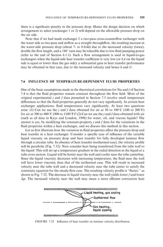

![PLATE HEAT EXCHANGER PRESSURE DROP 397
cuts and baffle spacings. In Chapters 8 and 9, we show how to obtain some of the input
data of this problem.
6.5 PLATE HEAT EXCHANGER PRESSURE DROP
Pressure drop in a plate heat exchanger consists of three contributions: (1) pressure drop
associated with the inlet and outlet manifolds and ports, (2) pressure drop within the core
(plate passages), and (3) pressure drop due to the elevation change for a vertical flow
exchanger. The pressure drop in the manifolds and ports should be kept as low as
possible (generally 10%, but may be as high as 25 to 30% or higher in some designs).
Empirically, it is calculated as approximately 1.5 times the inlet velocity head per pass.
Since the entrance and exit losses in the core (plate passages) cannot be determined
experimentally, they are included in the friction factor for the given plate geometry.
Although the momentum effect [see Eq. (6.28)] is negligibly small for liquids, it is also
included in the following p expression. The pressure drop (rise) caused by the elevation
change for liquids is given by Eq. (6.5). Summing all contributions, the pressure drop on
one fluid side in a plate heat exchanger is given by
p ¼
1:5G2p
np
2gci
þ 4fLG2
2gcDe
1
m
G2
þ 1
o
1
i
gc
mgL
gc
ð6:44Þ
where Gp
¼ m_ =ð=4ÞD2p
is the fluid mass velocity in the port, np is the number of passes on
the given fluid side, De is the equivalent diameter of flow passages (usually, De equals
twice the plate spacing), and o and i are fluid mass densities evaluated at local bulk
temperatures and mean pressures at outlet and inlet, respectively.
Example 6.3 A 1-pass 1-pass plate heat exchanger with chevron plates is being used to
cool hot water with cold water on the other fluid side. The following information is
provided for the geometry and operating conditions: number of flow passages 24 on
the hot-water side, plate width 0.5 m, plate height 1.1 m, port diameter 0.1 m, channel
spacing 0.0035 m, equivalent diameter 0.007 m, hot-water flow rate 18 kg/s, mean
dynamic viscosity 0.00081 Pa s, and mean density 995.4 kg/m3 for both manifolds and
core. The hot water is flowing vertically upward in the exchanger. The friction factor for
the plates is given by f ¼ 0:8Re
0:25, where Re ¼ GDe= is the Reynolds number.
Compute the pressure drop on the hot-water side.
SOLUTION
Problem Data and Schematic: The following information is provided:
np
¼ 1 Np
¼ 24 w ¼ 0:5m L ¼ 1:1m Dp
¼ 0:1m b ¼ 0:0035m
De
¼ 0:007m m_ ¼ 18 kg=s ¼ 0:00081 kg=m s ¼ 995:4 kg/m3
0:25
f ¼ 0:8Re
A typical plate heat exchanger is shown in Fig. 1.16.
Determine: The hot-water-side pressure drop for this plate heat exchanger.](https://image.slidesharecdn.com/fundamentalsofheatexchangerdesign-131001160835-phpapp01-141008073824-conversion-gate02/85/Fundamentalsofheatexchangerdesign-131001160835-phpapp01-562-320.jpg)

![PRESSURE DROP ASSOCIATED WITH FLUID DISTRIBUTION ELEMENTS 399
available for the core and that will also result in more uniform flow through the plate
passages.
6.6 PRESSURE DROP ASSOCIATED WITH FLUID DISTRIBUTION
ELEMENTS
Fluid flows into and out of the heat exchanger through pipes, ducts, or nozzles. These are
usually connected to manifolds, tanks, or headers for fluid distribution to the heat
exchanger flow passages. The pressure drop associated with these components usually
consists of wall friction, bend losses, sudden contraction and expansion losses, and
branch losses, depending on the geometry. When information on the friction factor is
not available, these pressure losses are generally presented in terms of velocity heads, as
in the first equality of Eq. (6.53), where the pressure loss coefficient K represents the
number of velocity heads. These pressure losses are summarized separately next.
6.6.1 Pipe Losses
The pressure drop associated with a pipe of constant cross section, due to wall friction, is
given by Eq. (6.29) as
p ¼ f
4L
Dh
u2
m
2gc
ð6:45Þ
where f is the Fanning friction factor, generally dependent on the Reynolds number and
flow cross-section geometry. In turbulent flow, f is also dependent on the surface rough-ness
of the pipe. Fluid mass density is evaluated at local bulk temperature and mean
pressure.
The Fanning friction factor as a function of Re and e=di
¼ e=Dh for a circular tube is
presented in Fig. 6.4. Here e is the surface roughness magnitude (average height) and
di
ð¼ Dh
Þ is the tube inside diameter. The results are valid for fully developed laminar and
turbulent flows. Notice that the surface roughness has no influence on the f factors in
laminar flow. If the ordinate of Fig. 6.4 is changed to 4f ¼ Darcy friction factor [see Eq.
(7.20)], the resulting figure is referred to as the Moody diagram. The turbulent flow f
factors of Fig. 6.4 are also valid for noncircular pipes provided that a proper value of the
hydraulic diameter is used in Eq. (6.45). The laminar friction factors f are dependent on
the cross-section geometry and are presented in Chapter 7. Further explanation of this
figure and the theory are presented in a subsection on Circular Tube with Surface
Roughness in Section 7.4.1.3.
6.6.2 Sudden Expansion and Contraction Losses
At the entrance of a heat exchanger, a pipe is generally connected to a manifold. Fluid
experiences a sudden expansion during the flow to the manifold. Similarly, it experiences
a sudden contraction while flowing from the exit manifold to the exit pipe. Sudden
expansion and contraction losses presented in Fig. 6.3 are applicable here. In heat
exchangers, these losses are associated with relatively large pipes, for which the flow is
turbulent. A review of Fig. 6.3 reveals that Ke is highest for Re¼1 for a given . By](https://image.slidesharecdn.com/fundamentalsofheatexchangerdesign-131001160835-phpapp01-141008073824-conversion-gate02/85/Fundamentalsofheatexchangerdesign-131001160835-phpapp01-564-320.jpg)


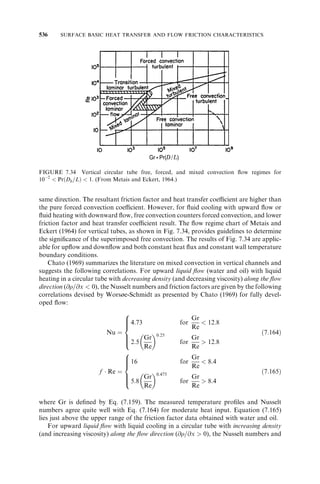

![When a fluid flows through a bend or a curve, it experiences a variation of centrifugal
force across the tube. This results in a pressure gradient between the outer wall
(maximum pressure) and the inner wall (minimum pressure) at a given cross section.
This results in a secondary flow, as shown at section AA in Fig. 6.5, superimposed on the
main flow. The frictional energy loss near the tube walls is thus increased and the pressure
drop is greater than that for the corresponding flow in a straight tube.
In the following formulation of expressions for the pipe bend pressure losses, it is
assumed that these losses are associated only with the pipe bend and the outlet pipe
section of Fig. 6.5. The pressure drop associated with a smooth straight inlet pipe section
of the bend is not included (but must be included when calculating the total pressure drop
associated with a heat exchanger having pipe bends) because it can be calculated straight-forwardly
[e.g., by using Eq. (6.29)] separately. If the bend follows another component
(bend, tee, etc.), the pressure loss associated with the inlet pipe section is already included
in Eq. (6.49) for specific lengths of the inlet pipe section specified in Sections 6.6.3.1
through 6.6.3.3.
The pressure drop associated with a bend may be represented by
pb
¼ Kb;t
u2
m
2gc
ð6:48Þ
where is the fluid density evaluated at local bulk temperature and mean pressure, um the
mean axial velocity (both and um evaluated at the entrance of the bend), and Kb;t is the
total pressure drop coefficient due to the bend. The total pressure drop for a bend consists
of two contributions: (1) the pressure drop for the bend due to the curvature effect,
the flow development effect in the outlet pipe, and the surface roughness effect, and (2)
the pressure drop associated with the outlet straight pipe of specified surface roughness.
The pressure loss coefficients Kb and Kf for these two contributions to the pressure drop
are strongly dependent on the flow Reynolds number. Thus,
Kb;t
¼ Kb
þ Kf
¼ Kb
þ f
4L
Dh
ð6:49Þ
404 HEAT EXCHANGER PRESSURE DROP ANALYSIS
FIGURE 6.5 Circular-cross-section pipe bend with a secondary flow pattern.](https://image.slidesharecdn.com/fundamentalsofheatexchangerdesign-131001160835-phpapp01-141008073824-conversion-gate02/85/Fundamentalsofheatexchangerdesign-131001160835-phpapp01-569-320.jpg)


![412 HEAT EXCHANGER PRESSURE DROP ANALYSIS
Example 6.6 Determine the pressure drop in a 908 miter bend using all the data given in
Example 6.5 for a 908 circular bend.
SOLUTION
Problem Data and Schematic: The schematic of the 908 miter bend is shown in Fig. E6.6
together with the input data.
di
di = 0.025 m
θb = 90°
e = 0.000025 m
L = 0.25 m
ρ = 997 kg/m2
μ = 0.000855 Pa • s
Flow
θb = 90°
L
FIGURE E6.6
Determine: Miter bend and downstream pipe pressure drop for the specified pipe.
Assumptions: The flow entering the bend is fully developed turbulent flow.
b *Analysis: Most of the information generated for the 908 circular bend is also applicable
here. For the miter bend, as mentioned in Section 6.6.3.3, Cdev
¼ 1 and K¼ 1:2 from
Fig. 6.12. From Example 6.4, CRe
¼ 1:48 and Crough
¼ 1:30: Hence,
Kb
¼ Kb *
CReCdevCrough
¼ 1:2 1:48 1 1:30 ¼ 2:31
and
Kb;t
¼ Kb
þ Kf
¼ Kb
þ f
4L
Dh
¼ 2:31 þ 0:0056 4 0:25m
0:025m
¼ 2:534
The pressure drop associated with the 908 miter bend is then
pb
¼ Kb;t
u2
m
2gc
¼ 2:534 997 kg=m3ð4:086m=sÞ2
2 1
¼ 21,090 Pa ¼ 21:09 kPa Ans:
Discussion and Comments: The pressure drop associated with the miter bend is 21.09 kPa;
for the same fluid and flow rates, the pressure drop for the circular bend is 4.62 kPa. Thus
the miter bend resulted in an increase in the pressure drop by about 4.5 times for this
example. Hence, whenever there is an option, a circular bend is generally preferred over a
miter bend for a lower pressure drop through the bend.
6.7 PRESSURE DROP PRESENTATION
For most heat exchanger surfaces, the core pressure drop [the core friction term in Eq.
(6.28)] for a given heat transfer surface is determined experimentally (using a ‘small size’](https://image.slidesharecdn.com/fundamentalsofheatexchangerdesign-131001160835-phpapp01-141008073824-conversion-gate02/85/Fundamentalsofheatexchangerdesign-131001160835-phpapp01-577-320.jpg)


![Since G ¼ m_ =Ao, we get from Eq. (6.58),
Gstd
¼ Gact
PRESSURE DROP PRESENTATION 415
std
act
ð6:60Þ
To match friction factors, use Eq. (6.54) and m_ = umAo to get
f ¼ p
2gc
u2
m
Dh
4L
¼ p
2gcA2o
m_ 2
Dh
4L
ð6:61Þ
Now let us match the standard and actual friction factors for a given geometry using
Eq. (6.61).
fstd
¼ fact
) pstdstd
m_ 2
std
¼ pactact
m_ 2
act
ð6:62Þ
Thus
pstd
¼ pact
act
std
2
m_ std
m_ act
ð6:63Þ
Substituting m_ std from Eq. (6.58) into Eq. (6.63), we get
pstd
¼ pact
act
std
2
std
act
ð6:64Þ
This is the most general relationship between pstd and pact that requires both density
and viscosity corrections, and should be used in all cases.
To illustrate the aforementioned effects of density and viscosity corrections, the
experimental pressure drop p with air as a function of the measured mass velocity G
is shown in Fig. 6.13a for a heat exchanger. The pressure drop p vs. mass velocity G
tests were conducted with air at six different inlet temperatures under isothermal condi-tions.
There is about a 17% spread in the experimental pressure drop over the tempera-ture
range covered. The same results are replotted in Fig. 6.13b with a traditional density
correction to a standard temperature of 158C (598F) [i.e., the pressure drop is corrected
using Eq. (6.66), and no correction is applied to the measured mass velocity G]. The
results collapse to about a 4% spread with the test temperature. Figure 6.13c shows the
recommended correction of density and viscosity [i.e., the pressure drop is corrected
using Eq. (6.64) and the mass velocity is corrected using Eq. (6.60)]. The results collapse
to a single curve, as expected from the foregoing theoretical basis.
However, in industry the viscosity correction in Eq. (6.64) is usually neglected
and only the density correction is applied. It can be rationalized as follows. When the
friction factor is constant (independent of the Reynolds number for turbulent flow, such
as in a rough pipe; see Fig. 6.4) or when f is not strongly variable for turbulent flow in a
smooth pipe, we do not need to match Restd and React as is done in Eq. (6.57). Hence, in
this case,
m_ std
¼ m_ act
ð6:65Þ](https://image.slidesharecdn.com/fundamentalsofheatexchangerdesign-131001160835-phpapp01-141008073824-conversion-gate02/85/Fundamentalsofheatexchangerdesign-131001160835-phpapp01-580-320.jpg)


![418 HEAT EXCHANGER PRESSURE DROP ANALYSIS
and Eq. (6.63) simplifies to
pstd
¼ pact
act
std
ð6:66Þ
To demonstrate that the viscosity correction is not significant for a turbulent flow (or
where the pressure drop is approximately proportional to the velocity square), isother-mal
tests similar to those of Fig. 6.13a are shown in Fig. 6.14a with air at three tempera-tures
on a perforated plate. The results are shown in Fig. 6.14b with the density
correction alone, and in Fig. 6.14c with the density and viscosity corrections together.
As it is found, whether only the density correction is applied (Fig. 6.14b) or both the
density and viscosity corrections are applied (Fig. 6.14c), the results of these tests collapse
to a single curve, as anticipated from the theoretical basis outlined above.
In most situations, whether or not f is constant is not known a priori, and therefore
Eq. (6.64) is recommended for correcting pact to pstd and Eqs. (6.58), (6.59), and
(6.60) for correcting _ m; _V
V, and G, respectively, for a plot of p vs. _ m; _V
V, or G at standard
conditions.
6.8 PRESSURE DROP DEPENDENCE ON GEOMETRY AND FLUID
PROPERTIES
Pressure drop in a heat exchanger core/matrix is dependent on some fluid properties and
geometrical parameters. Since the frictional pressure drop is the dominating contribution
to the core pressure drop, we use that term only for the analysis [i.e., Eq. (6.2) or (6.29)].
Substituting Ao
¼ DhA=4L from the definition of the hydraulic diameter, we get the
expression for p from Eq. (6.3) as
p ¼
1
D3h
#
1
2gc
ð4LÞ2
A
m_ ð f ReÞ
for laminar flow ð6:67aÞ
1
D3h
#
0:046
2gc
0:2
ð4LÞ2:8
A1:8 m_ 1:8
for turbulent flow ð6:67bÞ
8
:
Thus the pressure drop is proportional to D
3
h (for constant m_ , L, A, and fluid proper-ties).
For a circular tube, since A ¼ DhL, p of Eq. (6.67) is proportional to D
4
h and
D
4:8
h in laminar and turbulent flows respectively. Hence, based on Eq. (6.67),
p /
1
D3h
to
1
D4h
for laminar flow ð6:68aÞ
1
D3h
to
1
D4:8
h
for turbulent flow ð6:68bÞ
8
:
Reviewing Eq. (6.3) we find that p is proportional to L when Dh and Ao are
constant, and p is proportional to 1=Ao and 1=A1:8
o for laminar and turbulent flow
respectively when Dh and L are constant. In these comparisons, we also keep m_ and fluid
properties constant. Note that the surface area A is then not an independent variable
since A ¼ ð4AoLÞ=Dh:](https://image.slidesharecdn.com/fundamentalsofheatexchangerdesign-131001160835-phpapp01-141008073824-conversion-gate02/85/Fundamentalsofheatexchangerdesign-131001160835-phpapp01-583-320.jpg)
![p /
L;
1
Ao
SUMMARY 419
for laminar flow ð6:69aÞ
L;
1
A1:8
o
for turbulent flow ð6:69bÞ
8
:
From Eq. (6.67), we find that
p /
1
; for laminar flow ð6:70aÞ
1
; 0:2 for turbulent flow ð6:70bÞ
8
:
Thus, p is dependent on and as shown, but is not directly dependent on cp and k.
Finally, the dependence of the pressure drop on the surface geometry is given as
follows from the second equality of Eq. (6.29):
p / L
A2o
Dh
ð6:71Þ
for a specified fluid and its mass flow rate. Since the friction factors and Colburn factors
(or Nu) for enhanced heat transfer surfaces are higher than those for a plain surface, both
heat transfer rate and pressure drop for an enhanced surface will be higher than those for
a plain surface for a given fluid mass flow rate m_ and the same heat exchanger dimen-sions.
However, it is possible to maintain high-heat-transfer performance with the same
pressure drop (particularly in laminar flows) by properly choosing the heat exchanger
dimensions and surface geometry [i.e., the proper choice of L, Ao, and Dh in Eq. (6.71) so
that p remains the same]. Refer to Example 10.3 to gain some insight into this concept.
However, if the exchanger frontal area cannot be changed, one will end up with a larger
pressure drop with enhanced surface compared to that for the plain surface for a given
fluid flow rate. In that case (i.e., for a fixed frontal area), a plain unenhanced surface will
have a lower pressure drop but longer exchanger flow length (and hence larger volume
and mass of the exchanger) to meet the heat transfer requirement specified.
SUMMARY
In this chapter, important issues related to the pressure drop analysis and data presenta-tion
for a heat exchanger as a component are discussed with the following highlights.
. In a heat exchanger, the pressure drop (in addition to heat transfer) becomes an
important design consideration for gases in laminar, transition, and turbulent flow
and for highly viscous liquids in laminar flow. For other liquids, and particularly in
turbulent flow, the pressure drop is not as critical a design consideration as heat
transfer.
. Pressure drop associated with a heat exchanger is made up of two contributions:
(1) pressure drop associated with a core/matrix/heat transfer surface where heat
transfer takes place, and (2) pressure drop associated with flow distribution devices](https://image.slidesharecdn.com/fundamentalsofheatexchangerdesign-131001160835-phpapp01-141008073824-conversion-gate02/85/Fundamentalsofheatexchangerdesign-131001160835-phpapp01-584-320.jpg)


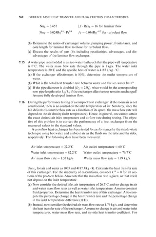


![BASIC CONCEPTS 435
beginning at x ¼ 0. The extent to which the viscous effects diffuse normally from the duct
wall is represented by the hydrodynamic boundary layer thickness v, which varies with
the axial coordinate x. In accordance with Prandtl’s boundary layer theory, the hydro-dynamic
boundary layer thickness divides the flow field into two regions: a viscous region
near the duct wall and an essentially inviscid region around the duct axis.
At x ¼ Lhy,{ the viscous effects have spread completely across the duct cross section.
The region 0 x Lhy is called the hydrodynamic entrance region, and the fluid flow in
this region is called the hydrodynamically developing flow. As shown in Fig. 7.6a, the axial
velocity profile in the hydrodynamic entrance region varies with all three space coordi-nates
[i.e., u ¼ uðx; y; zÞ]. For hydrodynamically developed flow, the velocity profile at a
given cross section becomes independent of the axial coordinate and varies with the
transverse coordinates alone [i.e., u ¼ uðy; zÞ or uðr; Þ]. The fully developed velocity
profile is essentially independent of type of the velocity profile at the duct inlet.
After the flow becomes hydrodynamically developed (x Lhy; Fig. 7.6a), suppose
that the duct wall temperature Tw is raised above the fluid entrance temperature Te (i.e.,
Tw Te). In this case, the local temperature changes diffuse gradually from the duct wall,
beginning at x ¼ Lhy. The extent to which the thermal effects diffuse normally from the
duct wall is denoted by the thermal boundary layer thickness t, which also varies with
0
the axial coordinate x. The t is defined as the value of y
(the coordinate measured from
the duct wall in Fig. 7.6) for which the ratio ðTw
TÞ=ðTw
Te
Þ ¼ 0:99. According to
Prandtl’s boundary layer theory, the thermal boundary layer thickness divides the flow
field into two regions: a heat-affected region near the duct wall and an essentially un-affected
region around the duct axis. At x ¼ Lth,{ the thermal effects have spread com-pletely
across the duct cross section. The region Lhy
x Lth is termed the thermal
entrance region, and the fluid flow in this region is called the thermally developing flow.
It may be emphasized that the thermally developing flow is already hydrodynamically
developed in Fig. 7.6a. As shown in this figure, in the thermally developing flow region,
the local dimensionless fluid temperature # ¼ ðTw
TÞ=ðTw
Te
Þ, varies with all three
spatial coordinates [i.e., # ¼ #ðx; y; zÞ].
For Lth
x 1 in Fig. 7.6a, the viscous and thermal effects have completely dif-fused
across the duct cross section. This region is referred to as the fully developed region.
The fluid flow in this region is termed the fully developed flow. In this region, the dimen-sionless
temperature # varies with the transverse coordinates alone, although the local
fluid temperature T varies with all three-space coordinates, and fluid bulk temperature
Tm varies with the axial coordinate alone. In the fully developed region, the boundary
conditions at the wall govern the convective heat transfer process so that the temperature
distribution is essentially independent of the duct inlet temperature and velocity distribu-tions.
{ The hydrodynamic entrance length Lhy is defined as the duct length required to achieve a maximum duct cross-section
velocity as 99% of that for a fully developed flow when the entering fluid velocity profile is uniform. The
maximum velocity occurs at the centroid for the ducts symmetrical about two axes (e.g., circular tube and
rectangular ducts). The maximum velocity occurs away from the centroid on the axis of symmetry for isosceles
triangular, trapezoidal, and sine ducts (Shah and London, 1978). For nonsymmetrical ducts, no general statement
can be made for the location of umax: There are a number of other definitions also used in the literature for Lhy.
{ The thermal entrance length Lth is defined, somewhat arbitrarily, as the duct length required to achieve a value of
local Nusselt number equal to 1.05 times the Nusselt number for fully developed flow, when the entering fluid
temperature profile is uniform. As discussed in Section 7.4.3.1, theoretically the Nusselt number is infinity at x ¼ 0
and reduces asymptotically to a constant value in fully developed flow.](https://image.slidesharecdn.com/fundamentalsofheatexchangerdesign-131001160835-phpapp01-141008073824-conversion-gate02/85/Fundamentalsofheatexchangerdesign-131001160835-phpapp01-600-320.jpg)
![436 SURFACE BASIC HEAT TRANSFER AND FLOW FRICTION CHARACTERISTICS
The fourth type of flow, called simultaneously developing flow, is illustrated in Fig.
7.6b and c. In this case, the viscous and thermal effects diffuse simultaneously from the
duct wall, beginning at x ¼ 0. Depending on the value of the Prandtl number Pr, the two
effects diffuse at different rates. In Fig. 7.6b, Pr 1 and v t, whereas in Fig. 7.6c,
Pr 1 and v t. This relationship among Pr, v and t is easy to infer from the
definition of the Prandtl number, which for this purpose can be expressed as
Pr ¼ =, a ratio of kinematic viscosity to thermal diffusivity. The kinematic viscosity
is the diffusion rate for momentum or for velocity in the same sense that the thermal
diffusivity is the diffusion rate for heat or for temperature change. For Pr 1, the
velocity profile (hydraulic) development is faster than the temperature profile (thermal)
development (so that Lhy Lth). For Pr 1, the velocity profile development is slower
than the temperature profile development (so that Lhy Lth). When Pr ¼ 1, the viscous
and thermal effects diffuse through the fluid at the same rate. This equality of diffusion
rates does not guarantee that the hydrodynamic and thermal boundary layers in internal
duct flows will be of the same thickness at a given axial location. The reason for this
apparent paradox lies in the fact that with Pr ¼ 1, the applicable momentum and energy
differential equations do not become analogous. In external laminar flow over a flat plate,
on the other hand, the energy and momentum equations do become analogous when
Pr ¼ 1. When the boundary conditions for the momentum and thermal problems are also
analogous, we get ¼ v
t for all values of x.
The region 0 x Lc in Fig. 7.6b and c is referred to as the combined entrance
region. It is apparent that the combined entrance length Lc is dependent on Pr.
For Pr 1, Lc
Lth, and for Pr 1, Lc
Lhy. It may also be noted that in the combined
entrance region, both the axial velocity and the dimensionless temperature vary with all
three space coordinates [i.e., u ¼ uðx; y; zÞ and # ¼ #ðx; y; zÞ where # ¼ ðTw; TÞ=
m
ðTw;m
Tm
Þ]. The region Lc
x 1 is the fully developed region, similar to the one
depicted in Fig. 7.6a with axially invariant uðy; zÞ and #ðy; zÞ, satisfying
@u
@x
xLhy
¼ 0
@#
@x
xLth
¼ 0 ð7:4Þ
In a fully developed laminar flow, the fluid appears moving by sliding laminae of infini-tesimal
thickness relative to adjacent layers. If a dye were injected at the centerline of a
tube in laminar flow of water, the colored streak will continue to flow without being
mixed at the tube centerline. While fully developed laminar flow is obtained for
Re 2300 for a smooth circular tube with smooth tube inlet, the actual value of the
Reynolds number to achieve/maintain fully developed or developing laminar flow
depends on the tube cross-sectional geometry, straightness, smoothness and constancy
of the cross section along the flow length, and the flow inlet geometry. We will discuss this
after we define the types of turbulent duct flows.
Turbulent Flow. The turbulent duct flows can also be divided into four categories: fully
developed, hydrodynamically developing, thermally developing, and simultaneously
developing. This division is identical to the one adopted for laminar duct flows in the
preceding subsection. However, there are some important differences:
. The hydrodynamic entrance length and the thermal entrance length for turbulent
duct flow are characteristically much shorter than the corresponding lengths in](https://image.slidesharecdn.com/fundamentalsofheatexchangerdesign-131001160835-phpapp01-141008073824-conversion-gate02/85/Fundamentalsofheatexchangerdesign-131001160835-phpapp01-601-320.jpg)
![BASIC CONCEPTS 437
laminar duct flow. Typical values of Lth=D are 8 to 15 for air and less than 3 for
liquids. Consequently, results for fully developed turbulent fluid flow and heat
transfer are frequently used in design calculations without reference to the hydro-dynamic
and thermal entrance regions. However, caution must be exercised in
using the fully developed results for the low Prandtl number liquid metals, since
the entrance region effects are quite pronounced for such fluids even in turbulent
duct flows (Lth=Dh
¼ 5 to 30, depending on Re and Pr).
. The turbulent flow development is preceded by the laminar boundary layer devel-opment
and through the transition region as shown in Fig. 7.3.
. Fully developed turbulent flow generally exists for Re 10,000 in a circular pipe.
For a sharp corner flow passage geometry such as a triangular passage, while the
flow is turbulent in the core region for Re 10,000, it is laminar in the sharp corner
region.
. The flow is fully developed turbulent for Re 10,000 for those flow geometries in
which turbulence is frequently generated within the flow passage geometry, such as
in a perforated fin exchanger or a corrugated plate heat exchanger. Typically, flow
is fully developed turbulent for Re 200 for plate heat exchanger geometries (see
Fig. 1.16) and for Re 100 on the shell side of a plate baffled shell-and-tube
exchanger.
Thus the Reynolds number at which fully developed turbulent flow can be achieved
depends on tube cross-section geometry, its variation along the flow length, the surface
roughness, and the flow inlet geometry.
Periodic Flow. In the regularly interrupted heat exchanger surfaces, such as a strip
fin surface, the conventional fully developed laminar or turbulent flow does not exit
[i.e., the velocity gradient of Eq. (7.4) is dependent on x]. Sufficiently downstream, the
velocity profile and the dimensionless temperature profile # ¼ ðTw; TÞ= Þ
m
ðTw;m
Tm
at a given cross section of each strip fin are identical:
uðx1; y; zÞ ¼ uðx2; y; zÞ #ðx1; y; zÞ ¼ #ðx2; y; zÞ ð7:5Þ
where x2
¼ x1
þ ‘, where ‘ is the length of one spatial period. This condition means that
Nux
ðx1; y; zÞ ¼ Nux
ðx2; y; zÞ ð7:6Þ
Usually, two to eight spatial repetitions are required to attain fully developed conditions
in a periodic geometry, with the exact number depending on the geometry and the
Reynolds number.
7.1.2.5 Flows with Separation, Recirculation, and Reattachment. The purpose of the
surface interruptions, such as in offset strip fins and louver fins, is to break the growth
of the boundary layer. This results in thin boundary layers and enhances the heat
transfer coefficient (usually accompanied by an increase in the friction factor).
However, an undesirable consequence of the surface interruption is often the separa-tion,
recirculation, and reattachment features in the flow, which results in more increase
in the f factor than in j or Nu. Consider, for example, the flow at the leading edge of a
fin of finite thickness. The flow typically encounters such a leading edge at the heat](https://image.slidesharecdn.com/fundamentalsofheatexchangerdesign-131001160835-phpapp01-141008073824-conversion-gate02/85/Fundamentalsofheatexchangerdesign-131001160835-phpapp01-602-320.jpg)


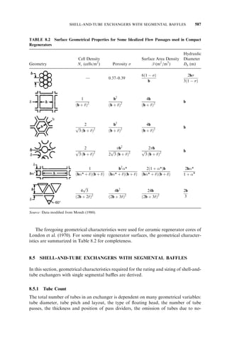


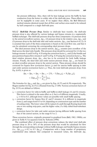


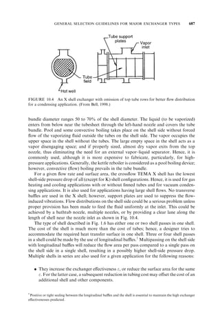


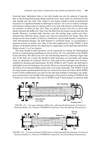


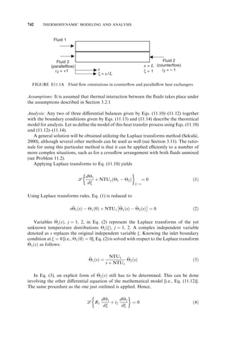


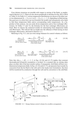


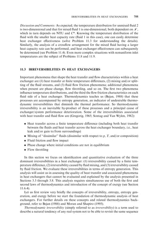


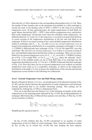


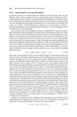


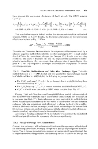
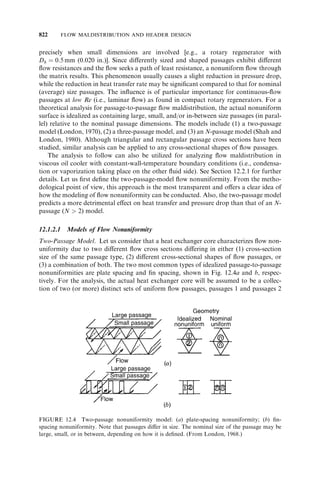


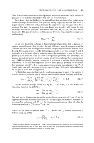


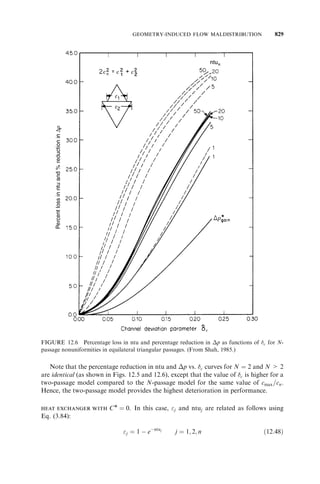


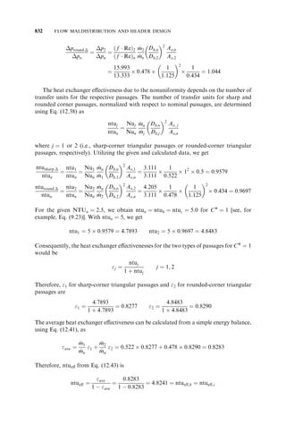


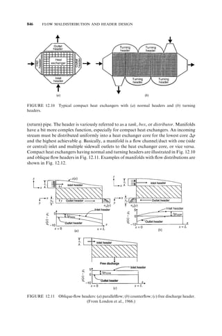

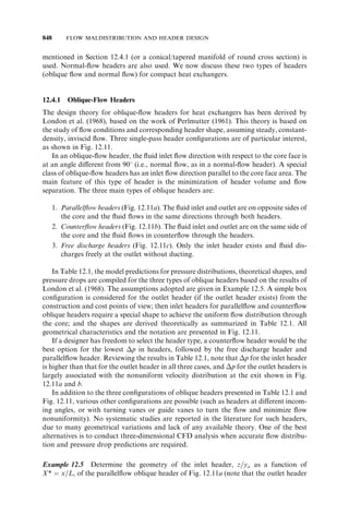


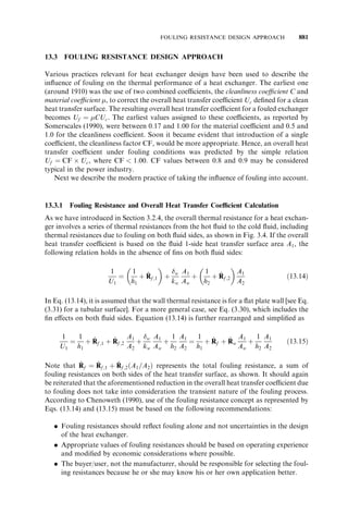


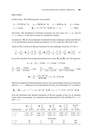


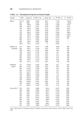


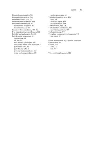

This document provides an overview of the textbook "Fundamentals of Heat Exchanger Design" by Ramesh K. Shah and Dušan P. Sekulic. The textbook covers topics related to heat exchanger classification, design methodology, thermal design theory, pressure drop analysis, heat transfer and flow characteristics, geometric characteristics, and design procedures. It provides the fundamental principles and methods for analyzing and designing various types of heat exchangers.


