Frequency domain behavior of S-parameters piecewise-linear fitting in a digital-wave framework

R E S E A R C H A R T I C L E
Frequency domain behavior of S-parameters piecewise-
linear fitting in a digital-wave framework
Piero Belforte1
| Domenico Spina2
| Maria Denise Astorino3
|
Giulio Antonini3
| Maurizio Ferrari1
1
Independent Researcher, Turin, Italy
2
Internet Technology and Data Science
Lab (IDLab), Department of Information
Technology, Ghent University-imec,
Ghent, Belgium
3
UAq EMC Laboratory, Dipartimento di
Ingegneria Industriale e dell'Informazione
e di Economia, Università degli Studi
dell'Aquila, L'Aquila, Italy
Correspondence
Piero Belforte, Independent Researcher,
Turin, Italy.
Email: piero.belforte@gmail.com
Abstract
This paper describes PWLFIT+, an extension to the frequency domain of
PWLFIT, a new paradigm in time-domain macromodeling for linear multiport
systems, based on a piecewise-linear (PWL) behavioral representation of the S-
parameters step response. While the impulse response of each S-parameter is
approximated as sum of delayed rectangles (rect) functions, its spectrum is
interpolated as sum of the corresponding delayed cardinal sine (sinc) func-
tions. Exploiting this correspondence, the model building is performed by an
iterative procedure where the PWL macromodels can be determined in order
to meet defined accuracy goals on the spectrum. At runtime, waves at
macromodels ports are calculated using the Segment Fast Convolution (SFC)
algorithm within the Digital Wave Simulator (DWS) framework. The proposed
method is characterized by its simplicity, stability, speed and scalability, all
features that are emphasized when it is used in the DWS framework. After an
analysis of the excellent numerical features of SFC in the Z-domain, clearly dif-
ferentiated with respect conventional macromodeling methods based on poles
and residues, two suitable application examples are presented to demonstrate
the unique features of PWLFIT+.
K E Y W O R D S
impulse response, S-parameters, step response, time- and frequency-domain
macromodeling
1 | INTRODUCTION
The macromodeling analysis aims to generate a model of complex electromagnetic linear systems using its characteriza-
tion at selected ports. This characterization can be in terms of transfer function in the frequency-domain, or in terms of
transient impulse response. In the first case, it can be obtained through measurements of a vector network analyzer
(VNA) or by numerical simulations using full-wave field or circuit solvers, while time-domain reflectometry
(TDR/TDT) and transient field or circuit solvers can be adopted in the latter case. While there is a vast literature for
macromodeling techniques using frequency-domain data,1–10
only few techniques have been developed over the years
for time-domain macromodeling. For example, the Time-Domain Vector Fitting (TD-VF) technique is introduced in
Received: 28 January 2021 Revised: 22 May 2021 Accepted: 21 June 2021
DOI: 10.1002/jnm.2934
This is an open access article under the terms of the Creative Commons Attribution-NonCommercial-NoDerivs License, which permits use and distribution in any
medium, provided the original work is properly cited, the use is non-commercial and no modifications or adaptations are made.
© 2021 The Authors. International Journal of Numerical Modelling: Electronic Networks, Devices and Fields published by John Wiley & Sons Ltd.
Int J Numer Model. 2021;e2934. wileyonlinelibrary.com/journal/jnm 1 of 22
https://doi.org/10.1002/jnm.2934

References 11,12 for the identification of the dominant poles of the structure using raw data transient excitations and
responses at the ports of the structure. An alternative time-domain macromodeling approach has been presented in Ref-
erences 13,14, where time-domain data are first partitioned into several intervals, then each interval is approximated
with a sum-of-exponentials, delayed in time. In References 15,16, the inverse fast Fourier transform (IFFT) of the sam-
pled frequency response of the multiport network under study is used to recover the corresponding time domain
impulse response. Taking advantage of its fast damping, a suitable decimation scheme of the impulse response can be
adopted in order to speed up the calculation of the time-domain convolution.
Recently, an automated version of PWLFIT,17–19
a well consolidated time-domain macromodeling technique for
general, linear multiport systems, has been presented in Reference 20. The PWLFIT method is based on a piecewise-
constant (PWC) model of the scattering parameters impulse response of the system under study, computed starting
from a piecewise-linear (PWL) fitting of the corresponding step response. Such behavioral time-domain models (BTM)
in PWC form are natively supported by the general Digital Wave simulation (DWS) framework as multiport scattering
elements.17,21–23
At runtime, the waves related to each S-parameter belonging to these elements are efficiently calcu-
lated via the Segment Fast Convolution (SFC) algorithm in alternative to the full convolution (FC), also supported.
Hence, the excellent speed, stability and scalability performance of DWS when dealing with standard circuit elements,
including Transmission Lines (TL), still apply for BTMs. The concept of BTM has been also extended to the so called
micro-behavioral models to be applied to 1D or 2D structures, such as lossy interconnects and power distribution
planes.24,25
The aim of this work is twofold. First, the previous analysis in Reference 20 is extended by defining the equivalent
representation of PWC models in both the frequency- and Z-domain. Then, PWLFIT+, the new extended version of
PWLFIT, capable to meet a specified accuracy target in a given frequency range, is described in detail. In particular,
PWLFIT+ is based on a time-domain rectangular (Rect) interpolation and on the corresponding frequency-domain car-
dinal sine (Sinc) interpolation. Note that, the function rect becomes sampled-rect in the discrete time, while in the
Z-domain the sinc becomes the aliased-sinc function, also known as Dirichlet function.26
Clearly, this is a fully innova-
tive and complementary approach with respect to conventional techniques based on transcendent (exponential and
trigonometric) functions in the time-domain and by rational functions in the complex frequency-domain, identified by
poles and residues.1
The paper is organized as follows. An overview of the PWLFIT modeling method is given in Section 2. The novel
frequency- and Z-domain representations of PWC models are presented in Section 3, while the extended PWLFIT+
modeling technique is described in Section 4. Two suitable application examples are presented in Section 5, while con-
clusions are drawn in Section 6.
2 | PWLFIT MACROMODELING
The standard S-parameters representation of a linear time invariant (LTI) system in the continuous time domain is:
b t
ð Þ ¼ s t
ð Þ*a t
ð Þ ¼
ðt
0
s t τ
ð Þa τ
ð Þdτ ð1Þ
where the S-parameters coincide with the reflected or transmitted waves when the incident ones are delta-function
pulses a τ
ð Þ ¼ δ τ
ð Þ.
The goal of the PWLFIT macromodeling technique20
is to compute a PWC model of each element of the S-
parameters impulse response. For a one-port system, this leads to:
s t
ð Þ ¼
X
N1
i¼1
rect Ai,ΔTi,Di
ð Þ ð2Þ
where N 1 is the number of segments of the PWC model, Ai its amplitude, Di its center, and ΔTi the temporal length
of each constant segment, as shown in Figure 1. For multiport systems, models in the form (2) can be computed for
each element of the S-parameters impulse response.20
2 of 22 BELFORTE ET AL.

Rather than computing directly the representation (2), the PWLFIT technique20
starts from the time-domain scatter-
ing step responses S t
ð Þ of the system under study, defined when the incident wave is defined as a step a τ
ð Þ ¼ u τ
ð Þ. Esti-
mating the step response rather than the impulse response via measurements (i.e., TDR/TDT) or numerical simulations
offers several advantages20
: for example, if the reference impedance of simulation is properly chosen, the time-domain
S-parameters step responses normally show relatively short duration before reaching steady state (DC) conditions.20
Then, a PWL model of the S-parameter step response is extracted via the automated PWLFIT procedure described in
Algorithm 1. In particular, starting from a set of tabulated data STw
including the transient step response, measured or
simulated at constant time step TIN defined in a suitable time window Tw, the desired time-domain PWL model SPWL t
ð Þ
with N 1 segments can be computed by identifying the breakpoints Ti,Si
ð Þ for i ¼ 1,…,N that define the extreme
points of each linear segment. Finally, the PWL model obtained so far can be refined in an extra post-processing step to
improve its accuracy without increasing the total number of breakpoints N.20
The PWL models before and after the
post-processing are referred as ONC (breakpoints on curve) and OFC (breakpoints off curve),20
respectively. Note that
the time coordinates Ti of these breakpoints are integer multiples of the time-step TIN , by construction. This dis-
cretization (temporal resolution) depending on TIN has also a significant effect on the related spectra, as discussed in
Section 5.
It is important to remark that, for multiport systems, each element of the step response scattering parameter matrix
Sr,c
, where r and c represent the row and column index, can be modeled separately and independently of the others,
even with different accuracy targets. However, the following condition
Sr,c
t ¼ 0
ð Þ ¼ 0, 8 r,c ð3Þ
must be satisfied to ensure the causality of the overall model. Furthermore, at steady-state (DC), that is, at time Tw for
which the residual transients of all Sr,c
are extinct, the relationships that bind Sr,c
to each other must be verified by the
DC analysis of the equivalent purely resistive network or from the TDR/TDT measurements. If these relationships are
not verified, the simulations that use the extracted model will likely incur into an error whose entity depends on the
magnitude of DC error affecting the S-parameters of the model.
The interested reader is referred to Reference 20 for a complete description of the PWLFIT method.
FIGURE 1 Three rectangles of a PWC model related to three consecutive samples (red crosses) of impulse response s t
ð Þ (blue solid line)
Algorithm 1
Automated PWLFIT method20
Result: PWL model with desired accuracy
Compute a PWL model starting from the two breakpoints tmin,Smin
ð Þ and tmax,Smax
ð Þ
while RMS S t
ð Þ,SPWL t
ð Þ
ð Þ ε do
Choose new ONC breakpoint: ti,Si
ð Þ ¼ max
t j
ð Þ
j S tj

SPWL tj

j
Update PWL model
end
Compute breakpoints OFC
BELFORTE ET AL. 3 of 22

3 | CONTINUOUS AND DISCRETE FREQUENCY-DOMAINS
REPRESENTATION OF PWC MODELS
3.1 | Laplace and Fourier domains formulation
The Laplace transform H s
ð Þ of (2) can be analytically calculated, leading to
H s
ð Þ ¼
X
N1
i¼1
Ai
s
es Di
ΔTi
2
ð Þ es Diþ
ΔTi
2
ð Þ

ð4Þ
Thanks to simple mathematical operations, it is possible to prove that Equation (4) for s ¼ jω becomes:
H ω
ð Þ ¼
X
N1
i¼1
2Ai
sin ωΔTi
2

ω
!
ejωDi
ð5Þ
which can be written as
H ω
ð Þ ¼
X
N1
i¼1
AiΔTisinc ω
ΔTi
2

ejωDi
ð6Þ
where sinc
ð Þ is the unnormalized sinc (cardinal sine) function. Hence, a PWC model of the impulse response is equiv-
alent in the frequency domain to a superposition of delayed sinc functions, whose phase is shifted by a term equal to
ejωDi
for i ¼ 1,…,N 1. The extension to general multiport systems is straightforward: each element of the impulse
response matrix can be represented via (4)–(6).
If a transfer function is expressed via (2), its spectrum can be exactly calculated using Equation (6).
3.2 | Spectrum calculation
The RectSinc transformation defined by (6) gives the exact spectrum of an impulse response composed by a sum of del-
ayed rectangles, obtained from the time derivative of the corresponding step response interpolated by a piecewise linear
function of time. It can be applied both to the extracted models and to input data containing the sampled step response.
The computation of spectrum (6) during the model extraction process will be described in Section 4, while the esti-
mation of the reference spectrum related to the input data will be discussed in the following. In this case, the time inter-
vals ΔTi are all equal to the TIN sampling interval of the Ns input samples. Furthermore, Equation (6) requires to
compute a sinc function for each frequency and for each rectangle, for a total of Nsinc = Nf Ns operations, where Nf
is the number of frequency samples. When Nsinc is in the order of tens of millions (or more), the RectSinc computation
can become computationally expensive. However, the RectSinc transform (6) of the input data can be efficiently calcu-
lated by applying the Fast Fourier Transform (FFT) implementation of DFT. Indeed, it is possible to derive a relation
between the DFT and the RectSinc, as follows.
Assuming that ΔTi ¼ TIN for i ¼ 0,1,2,…,Ns 1, the k-th sample of the DFT is given by:
Hk ¼
X
Ns1
i¼0
ΔSiej2π ki
Ns , k ¼ 0,1,2,…,Ns 1 ð7Þ
where
ΔSi ¼ AiΔTi ¼ AiTIN ð8aÞ
Di ¼
TIN
2
þiTIN ¼ TIN iþ0:5
ð Þ ð8bÞ

for i ¼ 0,1,2,…,Ns 1. Now, the RectSinc (6) is a continuous function of ω and, when computed at the k-th frequency
sample, it can be related to the DFT (7) as:
H ωk
ð Þ ¼
X
Ns1
i¼0
ΔSisinc ωk
TIN
2

ejωkTIN iþ0:5
ð Þ
¼
X
Ns1
i¼0
ΔSiejωkTIN i
sinc ωk
TIN
2

ejωk
TIN
2
¼
X
Ns1
i¼0
ΔSiej2π ki
Ns sinc ωk
TIN
2

ejωk
TIN
2
¼ Hksinc ωk
TIN
2

ejωk
TIN
2
¼ Hksinc
πk
Ns

ejπk
Ns
ð9Þ
From (9) it results that RectSinc H ωk
ð Þ at the discrete frequency k-th sample, can be derived from the DFT which can
be efficiently calculated by the FFT algorithm. Hence, it is possible to express the RectSinc transformation in (9) by
adopting a consistent notation with the DFT. From (9), it is also easy to verify that
lim
TIN !0
H ωk
ð Þ ¼ Hk ð10Þ
Hence, the RectSinc transformation reduces to the DFT as TIN ! 0. More information about the DFT to Rectsinc trans-
formation is available in Reference 27.
3.3 | Z-domain formulation
The transfer function of each PWC S-parameter can be obtained in both discrete-time and Z-domain as combination of
N 1 elementary blocks, each corresponding to a constant segment of its PWC model, as stated by (2) in time and by
(4) in the s-domain, respectively. Each segment block i corresponds to a specific Moving Average Filter (MAF).28
The
discrete-time impulse response of a MAF of order M is
hMAF n
ð Þ ¼
1
M
0 ≤ n ≤ M 1
0 otherwise
8

:
ð11Þ
where M is the number of averaged samples. The corresponding MAF transfer function is given by
HMAF z
ð Þ ¼
1
M
X
M1
n¼0
zn
¼
zM1
M zM z 1
ð Þ
½
ð12Þ
It is important to remark that the rational expression (12) contains a single pole of order M 1 at the origin of the
Z-plane and M 1 zeros on the unit circle.
In the following, it is assumed that the coordinates of all breakpoints extracted from the input data are linearly
interpolated at the time-step T chosen to run the simulation. The overall impulse response of the SFC can be expressed
as sum of all contributions of single PWC segments as:
hSFC n
ð Þ ¼
X
N1
i¼1
MiAihMAF i,n
ð Þ ð13Þ
where

ΔSi ¼ Si Si1 ð14aÞ
Mi ¼
ΔTi
T
ð14bÞ
Ai ¼
ΔSi
ΔTi
ð14cÞ
From (14), it is possible to write:
MiAi ¼
ΔSi
T
ð15Þ
In the Z-plane, Equation (13) becomes:
HSFC z
ð Þ ¼
X
N1
i¼1
ΔSi
T
zDSi
HMAFi
z
ð Þ ð16Þ
where
DSi ¼
Ti1
T
ð17Þ
From (12), Equation (16) can be written as:
HSFC z
ð Þ ¼
X
N1
i¼1
ΔSi
T
zMi1
Mi zMi z 1
ð Þ
½
zDSi
ð18Þ
Note that both Mi and DSi are integers, due to previous breakpoints interpolation according to time step T.
When the S-parameter step response contains a pure delay component, as usually happens in the case of intercon-
nects, this delay component can be separated from the rest of the response in order to avoid trivial numerical opera-
tions. If TD is the delay, (18) can be generalized as follows:
HDSFC z
ð Þ ¼ zD
HSFC z
ð Þ ð19Þ
where
D ¼
TD
T
ð20Þ
In (20), D is an integer because TD is discretized according to the time step T.
Figure 2 depicts the extraction flow and how each PWL segment and the related PWC rectangle are mapped in
DWS to implement the whole SFC structure described in the Z-plane by (18) and (19). A wave buffer of Mi cells is
defined for each segment along with a segment accumulator and a corresponding multiplicative coefficient Ai equal to
the slope of the related PWL segment.20
When the S-parameter step response includes a pure delay TD, this component
can be separated and implemented as a corresponding wave buffer in order to maximize the calculation speedup. Two
alternative options for pure delay processing are possible. The first, called ROUNDING, rounds the delay to the closest
integer D multiple of T. The second, called INTERPOLATION, implies an additional buffer cell and a linear combina-
tion of the two last cell values to calculate the delayed wave IND feeding the SFC block. The coefficients of this interpo-
lation are identified as KD0 and KD1 in Figure 2. This method, natively supported by DWS to deal with all the delays
present in the network under analysis, including TLs and controlled elements, gives more accurate results than the

simple rounding.21
It is also used for fractional delays processing in the digital sound synthesis29
and other Digital Sig-
nal Processing (DSP) fields.
If the interpolation method is used, Equation (19) becomes:
HDSFC z
ð Þ ¼ zD
KD0 þKD1z1

HSFC z
ð Þ ð21Þ
where
KD0 ¼ TD INT TD
ð Þ ð22aÞ
KD1 ¼ 1þINT TD
ð ÞTD ð22bÞ
where INT denotes the integer part of delay TD.
Thanks to (14) and (18), Equation (21) can be written as:
FIGURE 2 PWLFIT flow starting from a tabulated S-parameter step response including a TD delay and related segment fast convolution
(SFC) digital wave (DW) structure including input delay buffer options

HDSFC z
ð Þ ¼ KD z
ð Þ
X
N1
i¼1
ΔSi
ΔTi
z
ΔTi
T 1
z
ΔTi
T z 1
ð Þ
h izDSi
ð23Þ
where
KD z
ð Þ ¼ zD
KD0 þKD1z1

ð24Þ
The formulation in (23) corresponds to the wave structure depicted in Figure 2, where the multiplicative constants Ai
(segment slopes) are put in evidence. From (23) it is evident that the simulation time step T has only effect on the size
of each segment buffer and therefore on the number of zeros and of poles placed in the origin of Z-plane for each seg-
ment. This means that increasing T, the moving averages are calculated on about the same time window, but using a
decreasing number of samples.
From the considerations above, it is clear that the numerical properties of MAFs, already used in several DSP
applications,30
are fully exploited in the SFC implementation. First, the excellent numerical stability due to absence of
poles in the transfer functions, except at the origin of the Z-plane, as described by Equations (18), (19), (21) and (23).
Additionally, the rejection (smoothing) of both numerical and/or experimental noise affecting the SFC input signal,
and also the PWC segment parameters due to noisy input data. This smoothing is clearly due to MAF averaging features
and greatly contributes to the overall robustness of the PWLFIT method at runtime. This robustness is confirmed even
in case of a huge number (hundreds of thousands) of elements in the network under simulation, as proven by a great
number of practical applications.23,31
In this sense, the SFC is superior to the standard full convolution (FC) available
also to process BTM elements.20
The capability of taking into account all time delays, due to propagation phenomena
or other effects, at practically no computational cost and without affecting previous numerical properties, is another
important feature of the method. A final consideration is related to the simulation time step T, that affects the SFC
spectrum as stated by (23). The choice of T is a consequence of an overall trade-off between simulation speed and accu-
racy. As shown in detail by Reference 20, T greatly influences the SFC calculation and overall simulation speedup.
When dealing with complex networks, it is advisable to run at least two simulations at different T and to compare the
results in order to choose the best accuracy vs elapsed time ratio.
One last remark: the SFC method is general and it can be implemented in a wide range of software environments,
such as Matlab (Mathworks Inc., Natick, MA) or C++, as described in Reference 20. However, the full potential of SFC
can be optimally expressed when it is implemented in a DSP framework, as described in this section. Indeed, apart from
the simulation stability and the robustness to noisy input data discussed above, the DSP framework offers an accurate
transmission line modeling, the ability to process nonlinearities without iterations and the linear growth of processing
times with respect to the complexity of the network considered.19,20
4 | PWLFIT+
The PWLFIT+ procedure, able to deal with both time-domain (TD) or frequency-domain (FD) accuracy goals, is
described in the following.
As for the PWLFIT modeling presented in Section 2, the goal is to compute a time-domain PWL model of the S-
parameters step response S t
ð Þ via an iterative algorithm, where the number of breakpoints is gradually increased until
a desired accuracy target is reached. The initial data is a set of tabulated samples of DUT S-parameters step responses at
constant time step TIN on a limited time window Tw.
Based on the results presented in Section 3, it is now possible to define an error criteria to build the desired PWL
model that takes into account the accuracy in the estimation of the frequency response H ω
ð Þ of the system under study.
Indeed, if Hsinc ω
ð Þ is the frequency-domain representation of S-parameter impulse response obtained from a PWL
model SPWL t
ð Þ, the following error criteria can be defined:
• RMSTD: the RMS error between S t
ð Þ and the PWL model SPWL t
ð Þ;
• RMSFD ωl,ωh
ð Þ: the RMS error between the frequency response H ω
ð Þ and Hsinc ω
ð Þ, computed in the frequency
interval between ωl and ωh.

Hence, it is possible to extract a PWL model adopting three model building strategies: step-response driven
(RMSTD), spectrum-driven (RMSFD ωl,ωw
ð Þ), and a time/frequency domain mixed control, where both RMSTD and
RMSFD ωl,ωw
ð Þ must be satisfied. This extended domains model extraction is summarized in Algorithm 2, where εsr and
εspectr represent the desired accuracy targets in the time- and frequency-domain, respectively. The FRSC method in
Algorithm 2 is described in Section 4.1 and allows one to gain a significant speedup in the calculation of a PWL model,
when the spectrum-driven and mixed domain modeling strategies are adopted. Since the spectrum is computed starting
from tabulated data, it is important to consider the effect of the aliasing. In order to ensure an accurate estimation of
the spectrum, a frequency limit is suggested that is at least two orders of magnitude smaller than the inverse of TIN .
When dealing with multiport systems, each element of the S-parameter step response can be modeled indepen-
dently and different accuracy targets can be adopted for each element.
4.1 | Fast RectSinc spectrum calculation (FRSC)
If a spectrum-driven accuracy control criterion is used for new breakpoint selection, at each time the new breakpoint is
added during the iterative search, the corresponding spectrum should be computed again.
When a new breakpoint j is added between two existing breakpoints i1 and i, the current spectrum can be simply
updated as explained in Figure 3. The rectangle of amplitude Ai1,i and width ti ti1 is replaced by two rectangles
Ai1,j and Aj,i and width tj ti1 and ti tj, respectively. Hence, to obtain the updated spectrum, it is sufficient to sub-
tract the sinc function corresponding to the rectangle of amplitude Ai1,i and add two sinc functions, corresponding to
the new rectangles of amplitude Ai1,j and Aj,i.
Hence, when a new breakpoint j is added during the iterative fitting process in Algorithm 2, the new spectrum at
step j, defined as H f
ð Þj, can be calculated from the previous one H f
ð Þj1 as:
Algorithm 2
PWLFIT+ algorithm
Input data: TD S-parameters step-response
Choose Domain: TD or FD
if Domain = TD then
while RMSTD εsr do
Add a new breakpoint ONC: ti,Si
ð Þ ¼ maxt j
ð Þ j S tj

SPWL tj

j
Update PWL model
end
Result: TD-PWLFIT model with desired accuracy.
else if Domain = FD then
Choose frequency range: ωl, ωh
while RMSFD ωl,ωh
ð Þ εspectr do
Add a new breakpoint ONC: ti,Si
ð Þ ¼ maxt j
ð Þ j S tj

SPWL tj

j
Update PWL model
Update Hsinc ωl,ωh
ð Þ via FRSC (25)
end
Result: SD-PWLFIT model with desired accuracy.
else
TD/FD mixed control;
Result: TD/SD-PWLFIT model with desired εsr and εspectr accuracies.
end

H f
ð Þj ¼ H f
ð Þj1
sinc Ai1,i,ti ti1,Di1,i
ð Þ
þsinc Ai1,j,tj ti1,Di1,j

þsinc Aj,i,ti tj,Dj,i

ð25Þ
Indeed, in the standard procedure based on (6), at each iteration j the current spectrum is calculated as sum of all sincs
corresponding to all current segments. Hence, the required cpu-time for a K-step process can be estimated as
time ¼ timeRS þ2timeRS þ3timeRS
þjtimeRS þþN timeRS
¼ timeRS
X
K
j¼1
j
ð26Þ
where timeRS is the cpu-time required for the evaluation of a single rectsinc. When the feature described in (25) is
exploited, the cpu-time can be estimated as
time*
¼ timeRS þ2timeRS þ3timeRS
þ3timeRS þþ3timeRS
¼ 3timeRS K 3
ð Þ
ð27Þ
Hence, the speedup obtained exploiting the FRSC can be calculated as:
FSRCspeedup ¼
time
time*
¼
P
K
j¼1
j
3 K 1
ð Þ
ð28Þ
leading to a significant gain in terms of computational efficiency, even starting from a limited number (few dozens) of
segments K: from Equation (28) the speedup is equal to 9 for K ¼ 50, 17 for K ¼ 100, and 34 for K ¼ 200.
t
T T T
i-1 i
i
A
T - T
i
j
NEW Bkpt j
Bkpt i-1
Bkpt i
PWL
PWC
A
A
i-1,j
i,j
T - T j
j i-1
FIGURE 3 Effect of new breakpoint insertion on Fast RectSinc Spectrum Computation (FRSC)

4.2 | PWLFIT+ integration in the DWS framework
Figure 4 shows how PWLFIT+ can be used in the DWS modeling and simulation framework. An optional
oversampling step can be provided on the input data, if it is desirable to increase the aliasing-free bandwidth of the cal-
culated spectra. This optional step can be accomplished within the DWS framework by simulating a simple network
with the input samples feeding an ideal voltage generator. The oversampling time-step is defined by setting the number
of desired samples within the window Tw. In case of non-normalized TDR/TDT measurements, a correction (normali-
zation) of input data can be performed by means of an offset generator and a controlled voltage source of variable gain
added to the resampling network. As stated earlier, the time step T chosen to run the final DWS simulations depends
on the trade-off between simulation accuracy and speed; hence, T is usually different with respect the TIN time steps
related to all PWL models present in the network under analysis.20
DWS performs a preliminary linear interpolation at
FIGURE 4 DWS/PWLFIT+ modeling and simulation flow

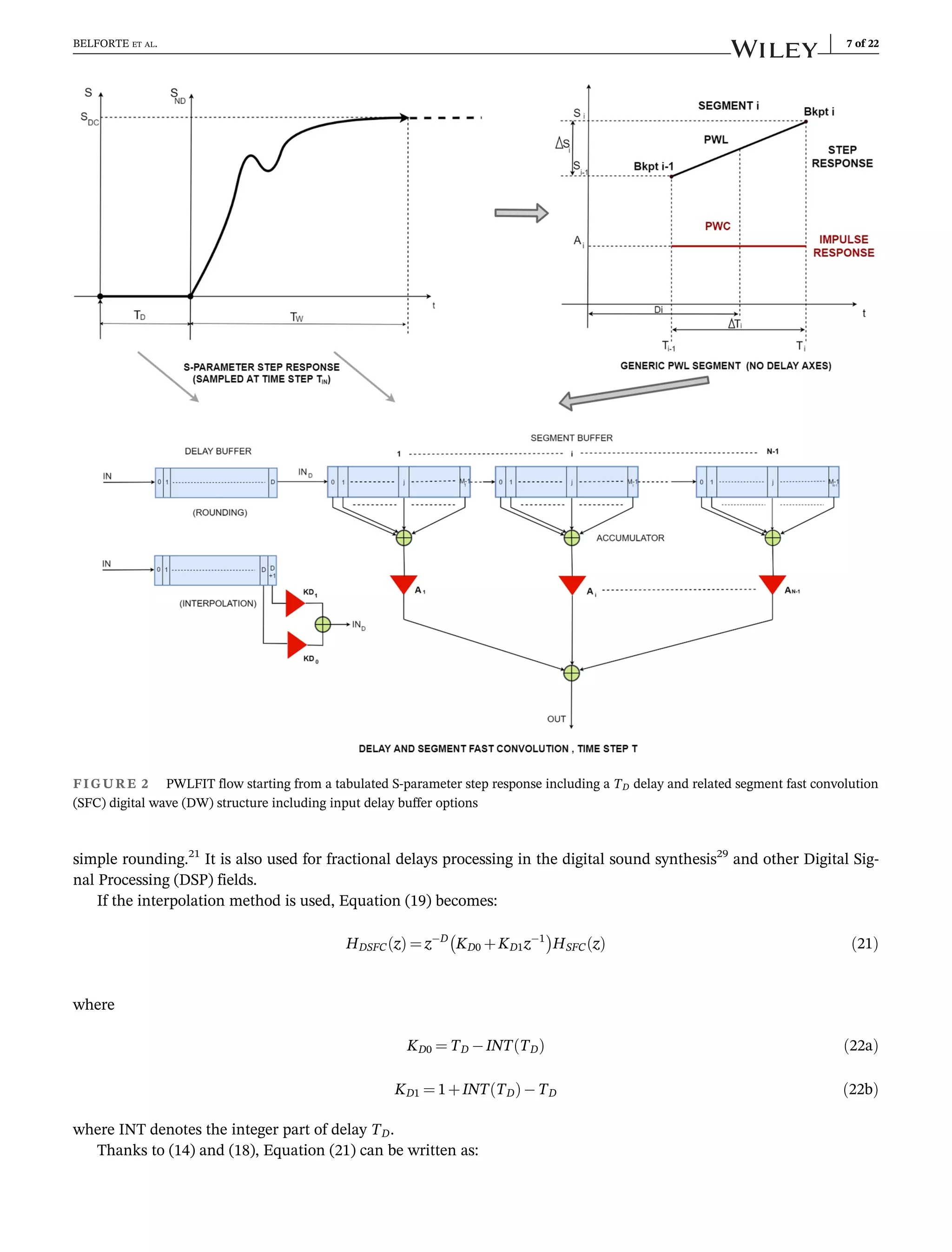
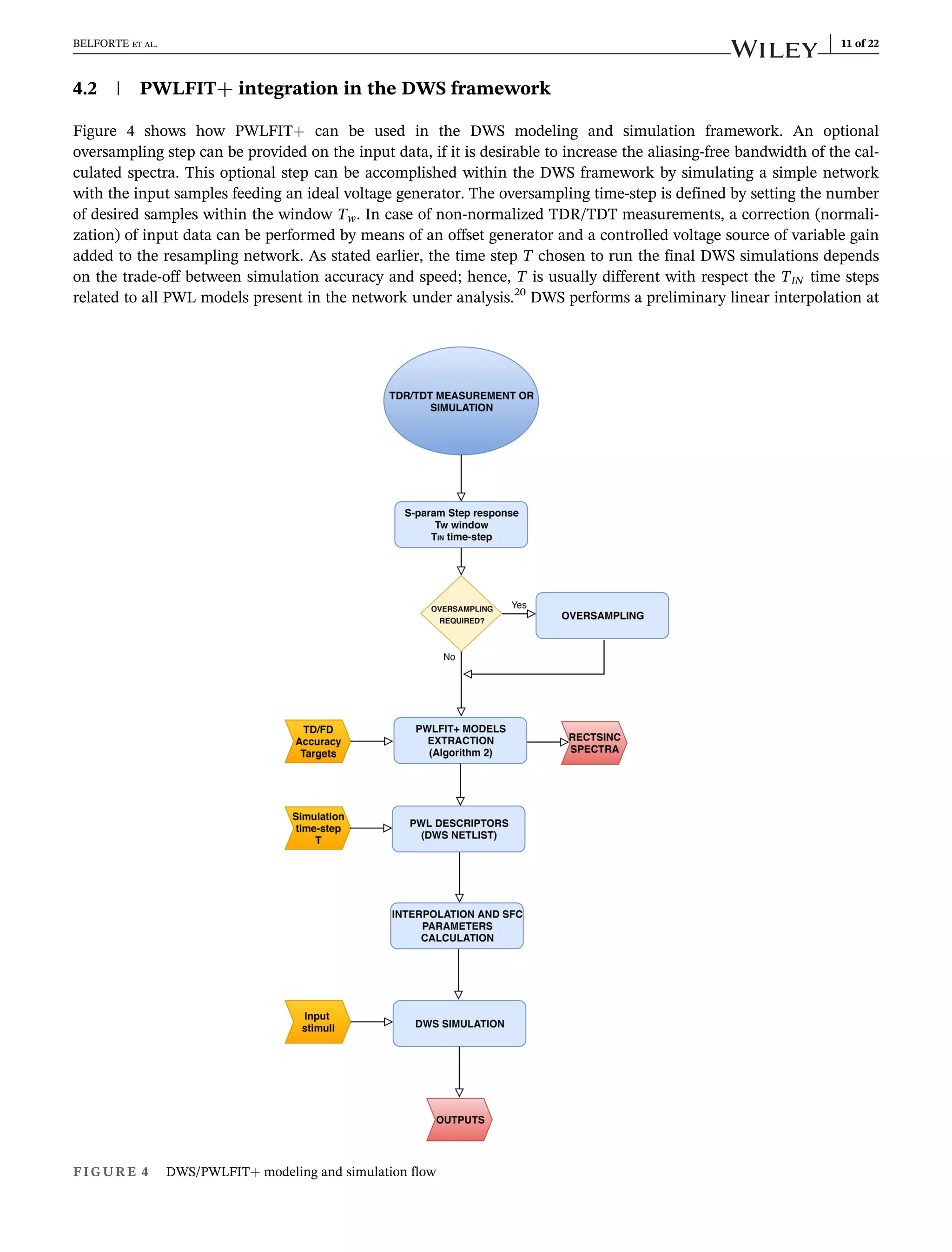
T of all PWL breakpoints included in the netlist, before computing the PWC models and run the simulation, as indi-
cated in Figure 4.
A final consideration on the impact of measurement noise on the performance of the proposed modeling method:
noise does not affect the stability of PWLFIT+ models, but can lead to a possible proliferation of breakpoints. Indeed,
when a high accuracy is chosen to model time-domain step responses (which corresponds to a low threshold εsr in
Algorithm 2), a large number of breakpoints can be needed to reduce the error due to the fast variations in time-domain
step responses caused by measurement noise. In case of TDR/TDT measurements, the noise can be controlled within
the instrument itself, usually by means of smoothing and/or averaging techniques. This happens at the expense of an
increase of the time required for acquiring the desired waveform, but this is no more an issue using modern instru-
ments. If the residual noise is still significant, it is possible to reduce its impact on the measured data by preprocessing
the acquired waveform using the same DSP framework (DWS) used for the simulations, using a suitable MAF or a cas-
cade of MAFs to perform a noise filtering on the samples. These MAFs can be easily described in the Spice-like syntax
of DWS by means of a controlled source with a PWL dynamic transfer functions.21
5 | NUMERICAL RESULTS
PWLFIT+ has been tested so far in several hundreds ideal and experimental applications. In the first case, the S-
parameter step-response of a capacitor has been obtained by DWS simulations. Then, the spectra calculated by PWLFIT
+ have been compared to continuous-frequency analytical formulas, when available, or to Spice AC analysis results.
The experimental examples have been carried out on several physical devices to assess the applicability of the method
to real applications. Both TDR and VNA instruments have been used to measure the S-parameters.
5.1 | One-port capacitor
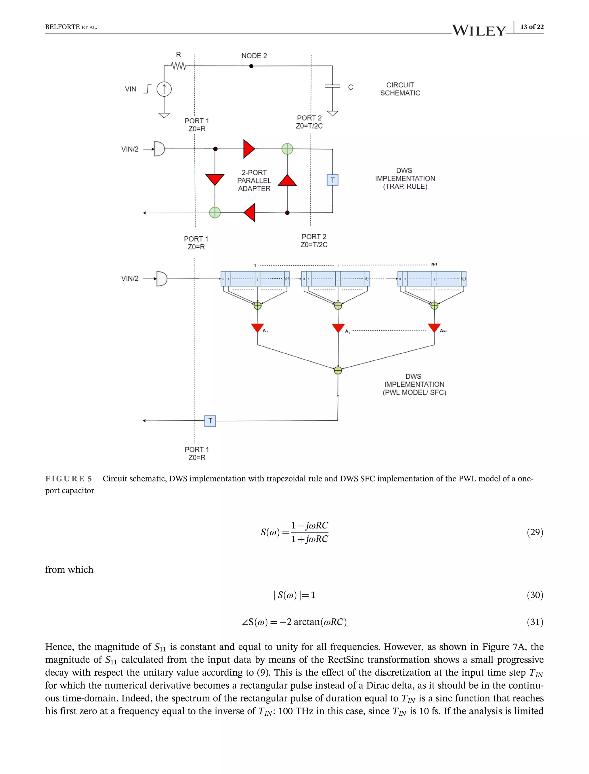
In this example, PWLFIT+ was applied to the reflected voltage step response, provided by DWS, of a simple circuit
composed of a capacitor with capacitance C ¼ 5 pF fed by a 2 V step generator of internal resistance R ¼ 50 Ω, as shown
at the top of Figure 5. The generator internal resistance R could be obviously chosen with a different value and repre-
sents an important degree of freedom in creating a PWL model. Figure 5 shows how DWS maps the RC circuit into a
Digital Wave equivalent. The capacitor's model consists of a simple one-step delay with impedance equal to T=2C
where T is the selected simulation time step. The incident wave step has an amplitude equal to VIN/2 (1 V in this case).
The connecting node 2 is implemented as a 2-port parallel adapter. The reflected wave's exponential behavior practi-
cally reaches the steady state value of 1 in 4 ns with a residual error of about 2e-7. A time window greater than 4 ns
obviously leads to a final sample closer to 1 at the expense of more samples. To minimize the integration error, a very
short time step of 0.1 fs was chosen to run the DWS simulation. The output data step was set to 10 fs, corresponding to
400 000 samples, in order to minimize the aliasing effects on the spectrum up to 1 THz.
The rms spectrum error target for PWLFIT+ was set to 0.001 in the range [1 MHz–1 THz] for the ONC model. The
computed PWL models consist of 56 breakpoints and the corresponding step responses are shown in Figure 6A.
The discrete-time impulse responses are calculated from the numerical derivative of their step responses, and are
represented in Figure 6B. The impulse response computed from the source data shows a dynamic range of more than
10 orders of magnitude (200 dB) and is perfectly linear on a logarithmic scale. The PWC approximations have a stair-
case behavior with 55 steps evolving around the source impulse response. Each stair step determines both the multipli-
cative coefficient Ai and buffer length of the corresponding SFC segment of the DWS behavioral block that implements
the PWL model (see Figure 2). In this ideal case, the standard DWS implementation of the capacitor is obviously com-
putationally far simpler and more accurate than the corresponding SFC wave structure. The required multipliers are
4 instead of 55, the adders are 2 instead of 55 accumulators and 1 adder of the SFC. Only one elementary delay is
required instead of a buffer of overall size equal to the ratio between the 4 ns window and the simulation time-step
T used at runtime.
PWLFIT+ calculates the spectra of both the input data and of the PWC models via Equation (6) and the results are
shown in Figure 7A for the magnitude and Figure 7B for the phase. The reflection coefficient in the frequency-domain
can be computed analytically in this case, as

S ω
ð Þ ¼
1jωRC
1þjωRC
ð29Þ
from which
j S ω
ð Þ j¼ 1 ð30Þ
∠S ω
ð Þ ¼ 2 arctan ωRC
ð Þ ð31Þ
Hence, the magnitude of S11 is constant and equal to unity for all frequencies. However, as shown in Figure 7A, the
magnitude of S11 calculated from the input data by means of the RectSinc transformation shows a small progressive
decay with respect the unitary value according to (9). This is the effect of the discretization at the input time step TIN
for which the numerical derivative becomes a rectangular pulse instead of a Dirac delta, as it should be in the continu-
ous time-domain. Indeed, the spectrum of the rectangular pulse of duration equal to TIN is a sinc function that reaches
his first zero at a frequency equal to the inverse of TIN: 100 THz in this case, since TIN is 10 fs. If the analysis is limited
FIGURE 5 Circuit schematic, DWS implementation with trapezoidal rule and DWS SFC implementation of the PWL model of a one-
port capacitor

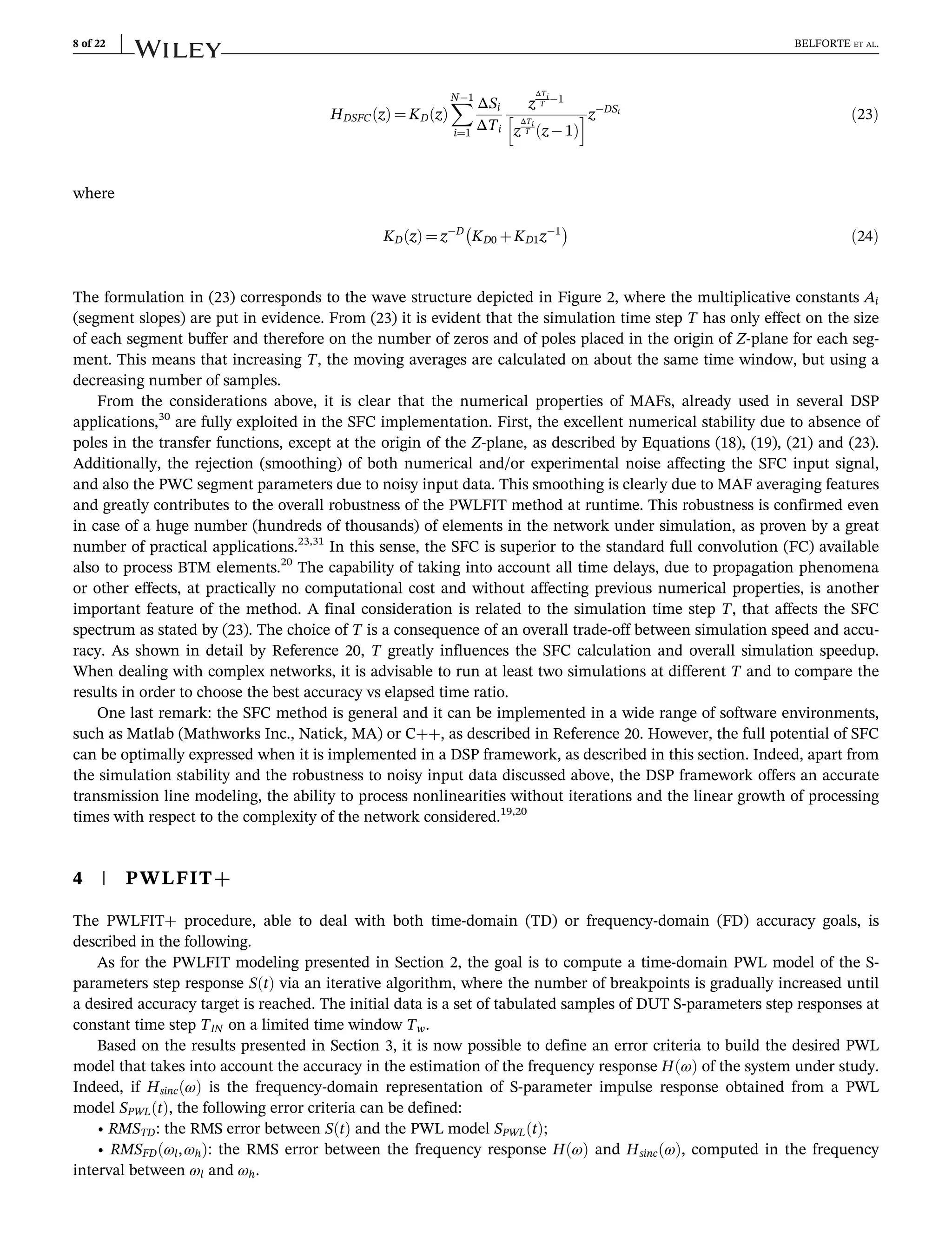
to 1 THz, as in our case, the decay with respect to 1 is in the order of 1e4. This small decay also affects the behaviors
of the extracted PWL models spectra, since the breakpoints have time coordinates multiples of TIN.27
In Figure 7A, the magnitude spectrum related to PWL models reaches a maximum of 1.006, while the input data
spectrum computed via (6) meets passivity constraints in the entire bandwidth considered. This is clearly due to the
PWL approximation of an ideal reactive (lossless) element and depends on both the input data time-step and the num-
ber of breakpoints. However, DWS simulations rely on the excellent numerical stability of both the MAFs of the SFC,
as discussed earlier, and of Digital Wave Networks, as clearly shown in Reference 32Ch. 15
and Reference 33. Note that,
the use of input data time-steps higher than 10 fs, for example, 1 ps, is the simplest way to avoid these passivity viola-
tions at the expense of a smaller model bandwidth. A study of the properties and effects of passivity of PWL models will
be carried out in future works, including the definition of methodologies to correct passivity violations during the itera-
tive breakpoints extraction.
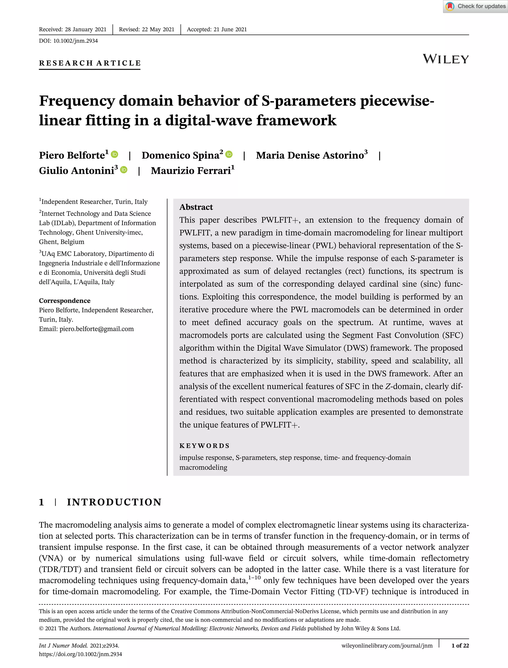
Figure 8 shows a test circuit where the extracted models of the capacitor are inserted in a fully reactive series reso-
nant circuit and compared to the ideal capacitor. The series adaptor AS is utilized to implement the trapezoidal rule for
the 10 nH inductor (Stub model) instead of the default TLM model (Link model). The time-step T chosen to run the
simulation is 200 fs, to get an equivalent bandwidth of 2.5 THz. As shown in the 3D (V,I,time) plot at the bottom of
Figure 8, passivity violations have no practical impact on DWS simulation stability. Only a progressive shift in both
0 1 2 3 4
Time [ns]
-1
-0.5
0
0.5
1
PWL
Model
Step
response
Input data
PWL OFC Model BP: 56
PWL ONC Model BP: 56
0 1 2 3 4
Time [ns]
105
1010
1015
Abs.
PWC
Model
Impulse
Response
Impulse response data
PWL OFC Model BP: 56
PWL ONC Model BP: 56
(A) (B)
FIGURE 6 (A) 56-breakpoints PWLFIT models of reflected wave step response for the 5 pF capacitor (R = 50 ohm). (B) Input data and
related PWC approximations of reflected wave impulse response for the 5 pF capacitor (absolute values)
FIGURE 7 (A) S11 magnitude spectra of the 5 pF capacitor. (B) S11 phase spectra of the 5 pF capacitor

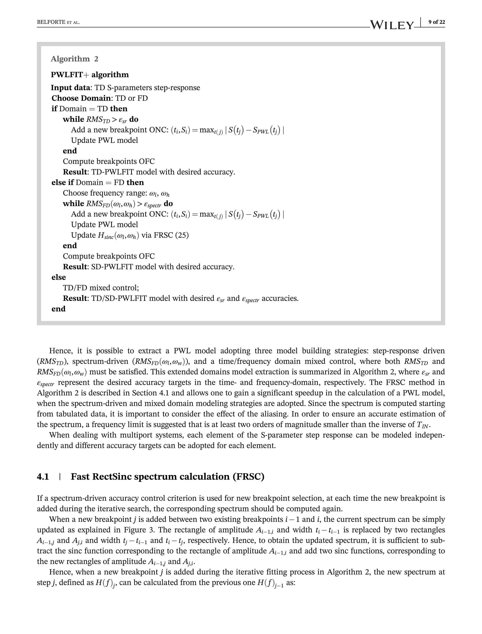
phase an amplitude is visible in the V,I trajectories of the models. Even by using a simulation time step T = 10 fs
(50 GHz bandwidth) and a VIN risetime of 10 fs, no stability issue is noticed.
5.2 | Multiband antennas for WiFi and LTE applications
Several samples of commercial antennas for WiFi and LTE applications have been characterized and processed by
means of PWLFIT+ both in standalone and coupled configurations. The antenna chosen for this example is a
multiband antenna for 3G and LTE/4G modems. The antenna is 19 cm long and is provided with a SMA connector and
an internal cable to allow rotation. The declared gain is 12 dBi for the 4G band. The antenna has been mounted on a
polycarbonate stand including a SMA adapter to allow the connection to the high-quality 50 Ω coax cable (Sucoflex
104, 1 m long). The fixture allows also the mounting of two antennas in a coupled configuration with an inter-axis of
35 mm as shown in Figure 9A. The complete setup for the coupled antennas is shown in Figure 9B.
The VNA used is a Keysight E5071C including the Time Domain option. The frequency range [9 kHz–6.5 GHz] has
been sampled with 20 001 samples. The calibration kit used is a hp85052C with 3.5 mm connectors. The calibration
has been performed at the SMA connectors ports of the stand in order to compensate all the effects of connecting cables
and SMA transitions. The measurements have been performed several times in order to verify that the presence of the
operator did not perturb the S-parameters spectrum. For the time-domain acquisitions the LOW-PASS STEP SIGNAL
mode has been chosen in order to get the TDR/TDT waveforms. The equivalent stimulus pulse rise time has been set to
minimum corresponding to 69 ps (0.45/FreqSpan).
FIGURE 8 Stability test circuit (series LC) for the PWL56 models of capacitor (top) and related 3D VI trajectories (bottom). Simulation
time-step T ¼ 200 fs

5.2.1 | Single antenna
The fixture used is shown in Figure 9A without the second antenna. Both the frequency and time-domain behaviors of
S11 have been obtained from the E5071C VNA (see Figure 9B without the second antenna). The time-domain response
is calculated by the VNA using the algorithms shown in References 34–36. Due to bandwidth limitation of the measure-
ment, some artifacts are present in the acquired time-domain waveform. The most evident one is the steady-state value
of S11 step response that does not converge to the correct value of 1. An empirical correction of these artifacts was done
by zeroing the samples for t ≤ 0 and compensating the slow decay with a linearly growing contribution in order to reach
the value 1 at t ¼ 200 ns, as shown in Figure 10. The interested reader can refer to34–36
for an overview of the techniques
to achieve the step or impulse response from the S parameters.
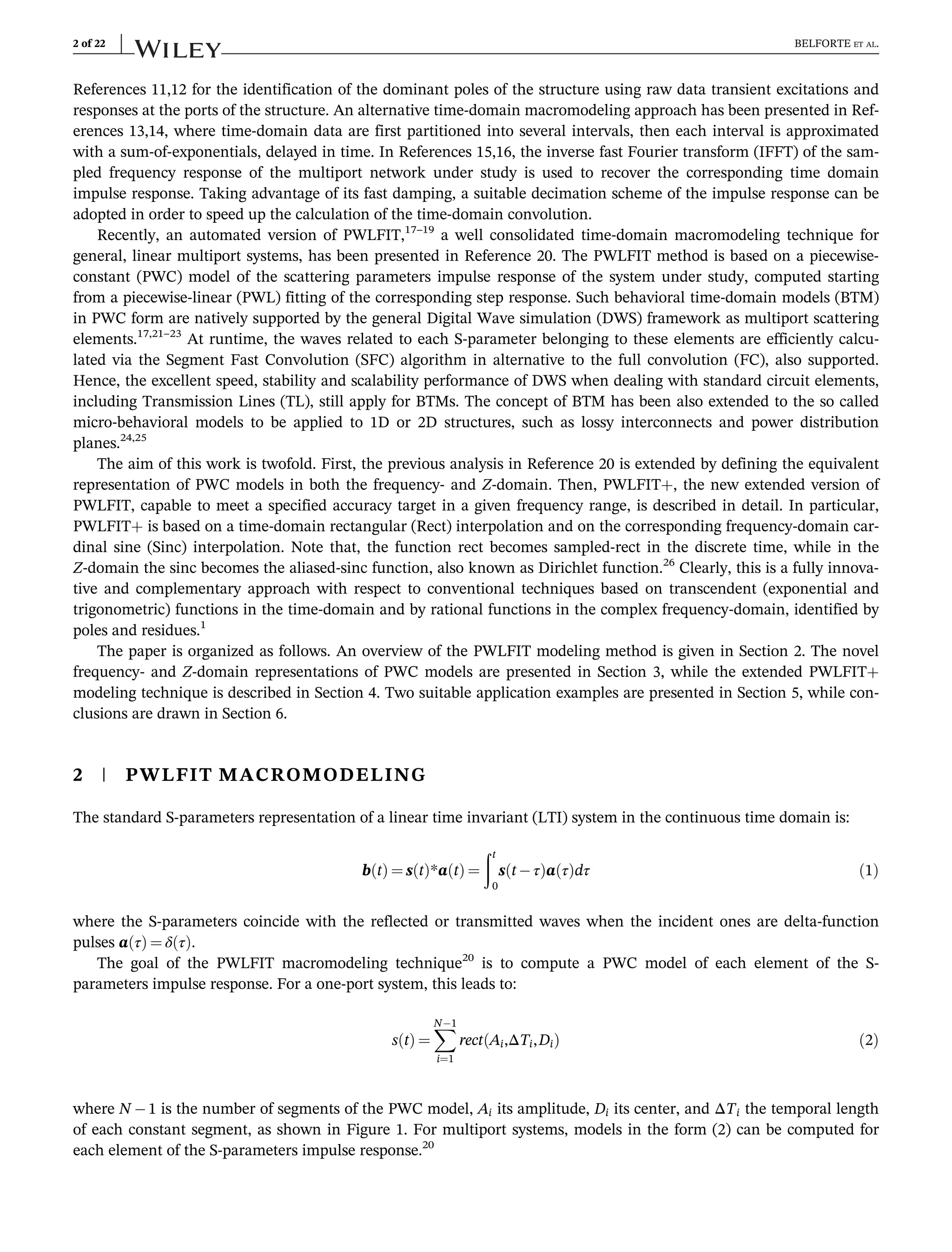
The PWLFIT+ procedure was then applied to the corrected waveform. The target rms spectrum error was set to
0.02 for the ONC model on a frequency interval between 10 MHz and 6.5 GHz, leading to ONC and OFC PWL models
with 164-breakpoints. The corresponding behaviors of the original and approximated PWC impulse responses (absolute
value) are shown in Figure 11A, while Figure 11B illustrates the behavior of both step-response and spectrum rms
errors of the ONC model versus the increasing number of breakpoints. In this case, the rms spectrum error is about one
order magnitude higher than the corresponding rms step-response error. The spectra calculated from both time-domain
FIGURE 9 (A) Fixture used for measurements on coupled multiband antennas. (B) Measurement setup using a E5071C VNA
0 10 20 30 40 50
Time [ns]
-0.2
0
0.2
0.4
0.6
0.8
1
1.2
S
11
Original data
Corrected data
FIGURE 10 S11 step response related to the single antenna. Original (solid blue) and corrected (dashed red) time-domain reflection
coefficient

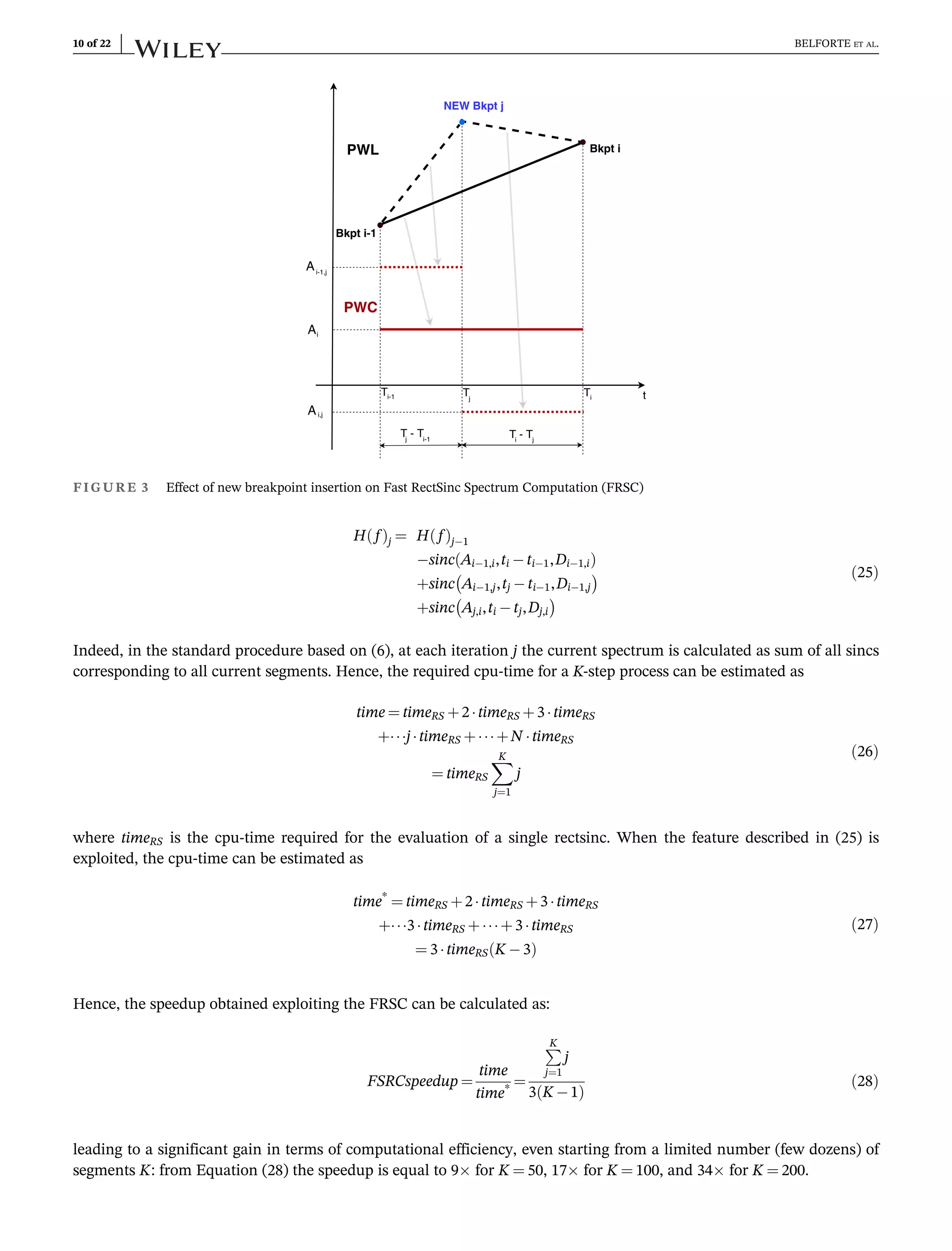
input data and PWL164 OFC model are compared to the original spectrum measured by the VNA and are shown in
Figure 12A for the module and Figure 12B for the phase. It can be pointed out that up to about 100 MHz the
reconstructed S11 module calculated by the instrument from time-domain data shows an amplitude slightly greater than
1 (about 1.02 maximum). This effect is due to low-frequency artifacts associated to the algorithms used inside the
instrument to perform the frequency to time conversion. As in the case of capacitor, these passivity violations do not
cause stability issues in the simulations performed.
5.2.2 | Coupled antennas
The fixture used in this case is shown in Figure 9A and the related setup in Figure 9B. Both the frequency spectrum
and the calculated time-domain step-responses of the four S-parameters have been acquired from the E5071C VNA.
The procedure followed to extract the PWL models for S11 and S22 is the same applied for S11 of the single antenna,
including the correction of the artifacts due to frequency to time conversion. The S21 step response as extracted from
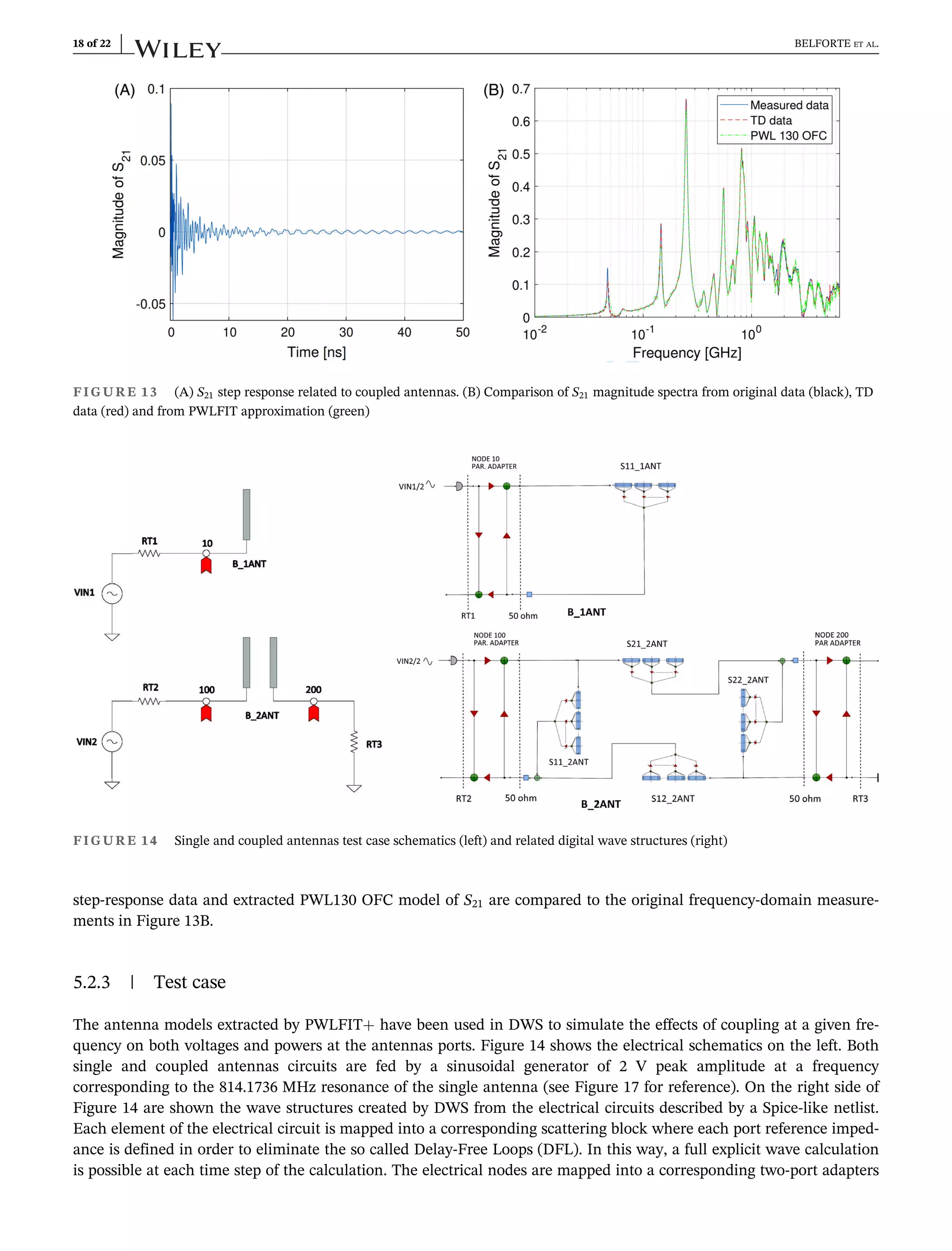
the VNA is shown in Figure 13A. The S12 parameter is identical to S21 according to reciprocity. The S21 time-domain
waveform generated by the VNA has been corrected by zeroing the values for t ≤ 0. No steady state correction is needed
in this case because no DC path exists between the coupled antennas. Spectra calculated by PWLFIT+ from both
FIGURE 11 (A) PWC approximation vs original impulse responses (FD error target = 0.02). (B) RMS errors vs number of breakpoints
(FD error target = 0.02)
10
-2
10
-1
10
0
Frequency [GHz]
10-1
100
Magnitude
of
S
11
RECTSINC OFC BP: 164
RECTSINC ONC BP: 164
RECTSINC Data
Measured Data
10
-2
10
-1
10
0
Frequency [GHz]
-4
-2
0
2
4
Phase
of
S
11
[rad] RECTSINC OFC BP: 164
RECTSINC ONC BP: 164
RECTSINC Data
Measured Data
(A) (B)
FIGURE 12 (A) Magnitude spectra of S11 for the single antenna. (B) Phase spectra of S11 for the single antenna

step-response data and extracted PWL130 OFC model of S21 are compared to the original frequency-domain measure-
ments in Figure 13B.
5.2.3 | Test case
The antenna models extracted by PWLFIT+ have been used in DWS to simulate the effects of coupling at a given fre-
quency on both voltages and powers at the antennas ports. Figure 14 shows the electrical schematics on the left. Both
single and coupled antennas circuits are fed by a sinusoidal generator of 2 V peak amplitude at a frequency
corresponding to the 814.1736 MHz resonance of the single antenna (see Figure 17 for reference). On the right side of
Figure 14 are shown the wave structures created by DWS from the electrical circuits described by a Spice-like netlist.
Each element of the electrical circuit is mapped into a corresponding scattering block where each port reference imped-
ance is defined in order to eliminate the so called Delay-Free Loops (DFL). In this way, a full explicit wave calculation
is possible at each time step of the calculation. The electrical nodes are mapped into a corresponding two-port adapters
FIGURE 13 (A) S21 step response related to coupled antennas. (B) Comparison of S21 magnitude spectra from original data (black), TD
data (red) and from PWLFIT approximation (green)
FIGURE 14 Single and coupled antennas test case schematics (left) and related digital wave structures (right)

whose multiplicative coefficients are calculated from the reference impedance at their ports. An additional one-step
delay is added at each B-element port to make the calculation full explicit. These additional delays are shown as small
squares in the wave structures of the figure and are electrically equivalent to a half time-step delay transmission line of
characteristic impedance equal to the reference impedance of the S-parameter block. This configuration has been simu-
lated by DWS with a time step of 5 ps on a 20 ns window. The elapsed time was 50 ms on a Hp Spectre 360 pc equipped
with an Intel Core I7 8705G 3.1 GHz CPU with 16 GB of RAM. Figure 15A,B show the simulation results in terms of
port voltages and powers, respectively. It is evident that the decrease of both voltage and power at the first antenna
when it is coupled with the second one. This effect is compensated by the voltage and power transferred to the second
antenna (green curves).
In order to compare the obtained results with a commercial tool, the single and coupled antennas have been simu-
lated also using the Advanced Design Systems (ADS).1
The simulated configuration is shown in the left side of
Figure 14, where the antennas are described by their tabulated scattering parameters. The time-domain simulations
performed by both DWS and ADS are in excellent agreement, as shown in Figure 16 for the coupled antennas case.
Similar results hold for the single antenna as well. The elapsed time for ADS was about 2.5 s. The calculation speedup
0 5 10 15 20
Time [ns]
-1.5
-1
-0.5
0
0.5
1
1.5
2
Voltage
[V]
1 Antenna
2 Antennas - Transmitting
2 Antennas - Receiving
(A)
0 5 10 15 20
Time [ns]
-5
0
5
10
15
20
Power
[W]
10-3
1 Antenna
2 Antennas - Transmitting
2 Antennas - Receiving
(B)
FIGURE 15 (A) Antenna port voltages, V(10) solid blue, V(100) dotted red, V(200) solid green. (B) Powers toward antennas, P(10) solid
blue, P(100) dotted red, P(200) solid green
0 5 10 15 20
Time [ns]
-1.5
-1
-0.5
0
0.5
1
1.5
2
Voltage
[V]
DWS
ADS
(A)
0 5 10 15 20
Time [ns]
-0.6
-0.4
-0.2
0
0.2
0.4
0.6
Voltage
[V]
DWS
ADS
(B)
FIGURE 16 (A) V(100) port voltage obtained in DWS (blue line) and ADS (red dashed line). (B) V(200) port voltage obtained in DWS
(blue line) and ADS (red dashed line)

is about 50 in favor of DWS for this simple test configuration. This speed advantage, typical of wave-domain environ-
ments, can be exploited in much more complex situations involving a large numbers of S-parameter macromodels. The
recent availability of TDRs with signal to noise ratio comparable to VNAs in the full frequency range (40 GHz)2
paves
the way for full time-domain simulation of complex RF and microwave systems. This result can be achieved directly
without the need of the artifact correction necessary when using tabulated frequency-domain data.
5.2.4 | TDR measurements
The antenna measurements have been also performed using a CSA803C TDR/TDT equipped with two 17.5 ps rise-time,
SD24 generator/sampling heads (20 GHz equivalent bandwidth). The fixture used was still the one shown in Figure 14,
but the surrounding environment was different. The procedure followed for the model extraction includes a DWS
oversampling and normalization step as shown in Figure 4. Note that no correction of artifacts due to frequency-to-time
conversion is needed in this case. However, at the highest frequencies the TDR spectra are affected by a signal to noise
ratio lower than the corresponding VNA measurements, but the effect of this noise is significantly smoothed thanks to
SFC features. The extracted PWL models have been used in the previously shown Test Case. Despite the differences of
instrument, environment and pre-processing procedures, the time-domain waveforms are in good agreement with the
corresponding ones obtained by the VNA, as shown in Figure 17.
6 | CONCLUSIONS
System Identification and Digital Signal Processing are both well-known but distinct disciplines. Communication
between them has been very rare. Filling this communication gap leads to brand new paradigms in modeling and simu-
lation methods featuring important advantages with respect to conventional techniques. An example is the DWS frame-
work, that applies the Wave Digital Filtering (WDF) concepts to general circuit and system simulation by mapping the
network under analysis into a DSP emulative model (Digital Wave Network, DWN) that is built up connecting together
scattering blocks related to circuital elements and nodes. Another example is the PWLFIT multi-port S-parameter mac-
romodeling technique, supported in DWS by BTM blocks. PWLFIT is based on a PWL fitting of the S-parameters step
response to build up the desired macromodel. At runtime, PWLFIT models can be processed by an efficient and stable
algorithm called Segment Fast Convolution, in alternative to the full convolution. This work has demonstrated how the
automated PWLFIT+ extension to the frequency domain, based on the RectSinc transformation, is very effective to
build up robust macromodels fulfilling a given accuracy target on an assigned frequency range. An efficient RectSinc
spectrum calculation (FRSC) algorithm provides a significant speedup during the iterative breakpoints identification
0 5 10 15 20
Time [ns]
-1.5
-1
-0.5
0
0.5
1
1.5
2
Voltage
[V]
CSA V(100)
CSA V(200)
E5071C V(100)
E5071C V(200)
FIGURE 17 Comparison of port voltages of the Test Case obtained using models based on CSA803C (TDR) and EN5071C (VNA)
measurements

process, while the analytical relationship between RectSinc and DFT (FFT) can be used to efficiently compute the spec-
tra of the tabulated input data. The robustness of the SFC, based on the summation of segment MAFs scaled in ampli-
tude on the basis of segment slope, leads also to a reduced sensitivity to both numerical and instrumental noise
affecting the input data. This property is enhanced by the distributed structure of the DWN model. This is a fundamen-
tal distinction with respect conventional methods based on Nodal Analysis (NA). Accurate time delays processing with-
out negative effects on computational cost and numerical stability is another unique feature of the method. Excellent
scalability in terms of both accuracy and number of ports of the extracted macromodel are also provided. Simulation
time step is the key parameter to achieve a desired speed/accuracy tradeoff. PWLFIT+ is applicable to data obtained
from electromagnetic or circuital simulators, including DWS, and from TDR and VNA measurements. Hence, the pro-
posed method can efficiently cover RF and microwaves applications in addition to SI/PI/EMC, where it has been suc-
cessfully applied for more than three decades.
ACKNOWLEDGMENTS
The authors wish to thank Giancarlo Guaschino for his development of DWS 9.0, the enhanced-accuracy version of
DWS including also up to 500 breakpoints per PWL description.
DATA AVAILABILITY STATEMENT
Data available on request from the author.
ORCID
Piero Belforte https://orcid.org/0000-0003-1775-8654
Domenico Spina https://orcid.org/0000-0003-2379-5259
Giulio Antonini https://orcid.org/0000-0001-5433-6173
ENDNOTES
1
Keysight Technologies, CA, USA.
2
See for example: TELEDYNE/LECROY https://teledynelecroy.com/oscilloscope/high-speed-interconnect-analyzer.
REFERENCES
1. Gustavsen B, Semlyen A. Rational approximation of frequency domain responses by vector fitting. IEEE Trans Power Del. 1999;14(3):
1052-1061.
2. Deschrijver D, Mrozowski M, Dhaene T, Zutter DD. Macromodeling of multiport systems using a fast implementation of the vector
fitting method. IEEE Microw Wirel Compon Lett. 2008;18(6):383-385.
3. Chung JH, Cangellaris AC. Fast rational function fitting of broadband multi-port responses via repeated random sampling. Proc. of IEEE
20th Conference on Electrical Performance of Electronic Packaging and Systems. San Jose, CA; IEEE; 2011. https://doi.org/10.1109/
EPEPS.2011.6100183
4. Kabir M, Khazaka R. Order selection for Loewner matrix based macromodels for accurate macromodeling of distributed high-speed
modules from limited number of full-wave S-parameter data. Proc. of IEEE 18th Workshop on Signal and Power Integrity (SPI). Ghent,
Belgium; IEEE; 2014. https://doi.org/10.1109/SaPIW.2014.6844546
5. Grivet-Talocia S, Gustavsen B. Passive Macromodeling: Theory and Applications. Hoboken, NJ: Wiley Series in Microwave and Optical
Engineering; 2015.
6. Fotyga G, Rewienski M, Mrozowski M. Wideband macromodels in finite element method. IEEE Microw Wirel Compon Lett. 2015;25(12):
766-768. https://doi.org/10.1109/LMWC.2015.2495192
7. Passos F, Ye Y, Spina D, et al. Parametric macromodeling of integrated inductors for RF circuit design. Microw Opt Technol Lett. 2017;59
(5):1207-1212.
8. Carrera-Retana LE, Rimolo-Donadio R, Schuster C. Efficient construction of interconnect passive macromodels through segmented
analysis. Proc. of IEEE 27th Conference on Electrical Performance of Electronic Packaging and Systems (EPEPS). San Jose, CA; IEEE;
2018. https://doi.org/10.1109/EPEPS.2018.8534236
9. De Ridder S, Deschrijver D, Spina D, Vande Ginste D, Dhaene T. Statistical modeling of frequency responses using linear Bayesian vec-
tor fitting. Int J Numer Model-Electron Netw Device Fields. 2020;33(6):e2762.
10. Rangel A, Gallego A, Vega F, Becerra J, Campos R. Parametric macromodeling of the coupling between two nearby parabolic antennas
using the Cauchy method. Proc of IEEE International Conference on Computational Electromagnetics (ICCEM). Singapore; IEEE; 2020.
https://doi.org/10.1109/ICCEM47450.2020.9219408
11. Grivet-Talocia S. Package macromodeling via time-domain vector fitting. IEEE Microw Wirel Compon Lett. 2003;13(11):472-474. https://
doi.org/10.1109/LMWC.2003.819378

12. Lei C, Wong N. Efficient linear macromodeling via discrete-time time-domain vector fitting. Proc. of 21st International Conference on
VLSI Design (VLSID 2008). Hyderabad, India; IEEE; 2008. https://doi.org/10.1109/VLSI.2008.12
13. Charest A, Saraswat D, Nakhla M, Achar R, Soveiko N. Compact macromodeling of high-speed circuits via delayed rational functions.
IEEE Microw Wirel Compon Lett. 2007;17(12):828-830. https://doi.org/10.1109/LMWC.2007.910468
14. Charest A, Nakhla M, Achar R, Saraswat D, Soveiko N, Erdin I. Time domain delay extraction-based macromodeling algorithm for long-
delay networks. IEEE Trans Adv Packag. 2010;33(1):219-235.
15. Schutt-Ainé JE, Goh P, Mekonnen Y, et al. Comparative study of convolution and order reduction techniques for Blackbox mac-
romodeling using scattering parameters. IEEE Trans Compon Packag Manuf Technol. 2011;1(10):1642-1650. https://doi.org/10.1109/
TCPMT.2011.2163308
16. Goh P, Schutt-Ainé JE. Improving fast S-parameter convolution by optimising reference impedance. Electron Lett. 2014;50(18):1290-
1292.
17. Belforte P. Sprint and Sights Applications. HDT; 1989. https://doi.org/10.13140/RG.2.1.3792.5605.
18. Belforte P. Sprint and Sights Appications 1990. HDT; 1990. https://doi.org/10.13140/RG.2.2.11885.33764.
19. Belforte P. Digital wave simulation of lossy lines for multi-gigabit applications. IEEE Electromagnetic Compatibility Magazine. 2016;5 (2):
48-55. http://dx.doi.org/10.1109/memc.0.7543950.
20. Belforte P, Spina D, Lombardi L, Antonini G, Dhaene T. Automated framework for time-domain piecewise-linear fitting method based
on digital wave processing of S-parameters. IEEE Trans Circuits Syst I-Regul Pap. 2020;67(1):235-248. https://doi.org/10.1109/TCSI.2019.
2944198
21. Belforte P, Guaschino G. DWS 9.0: Digital Wave Simulator. 2020. https://doi.org/10.13140/RG.2.2.11489.66407/1.
22. Sisto R. SPRINT: a DSP-based electrical simulator. Proc. of IASTED International Symposium. Lugano, Italy; IASTED; 1990.
23. Belforte P. SWAN-DWS Project. Research Gate; 2017. https://www.researchgate.net/project/SWAN-DWS.
24. Belforte P. Modeling and Simulation of P.C.B. Power and Ground Distribution Planes. HDT; 1993. https://doi.org/10.13140/2.1.1765.2006.
25. Belforte P. Vector vs Piecewise-Linear Fitting for Signal and Power Integrity Simulation. PBLAB; 2015. https://doi.org/10.13140/RG.2.1.
4150.5129.
26. Smith JO. Spectral Audio Signal Processing. San Diego, California: W3K Publishing; 2011.
27. Belforte P. Rectsinc vs DFT(FFT) Transformation. PBLAB; 2020. https://doi.org/10.13140/RG.2.2.10713.88161/1.
28. Polikar R. FIR and IIR Transfer Functions. Rowan University. 2010. https://www.astro.rug.nl/vdhulst/SignalProcessing/Hoorcolleges/
college07.pdf
29. Smith J. Interpolated Delay Lines, Ideal Bandlimited Interpolation, and Fractional Delay Filter Design. 2020. CCRMA: MUS420 Lec-
ture 4A.
30. Smith SW. Digital Signal Processing – A Practical Guide for Engineers and Scientists. Moving Average Filter. Burlington, MA: Elsevier Sci-
ence; 2002.
31. Belforte P. DWS-PWLFIT-PROJECT. Research Gate; 2018. https://www.researchgate.net/project/DWS-PWLFIT.
32. Smith SW. The scientist and engineer's guide to digital signal processing. San Diego, California: California Technical Publishing; 2002.
33. Bilbao S, Smith JOS. Finite difference schemes and digital waveguide networks for the wave equation: stability, passivity, and numerical
dispersion. IEEE Trans Speech Audio Process. 2003;11(3):255-266.
34. Keysight Application Note. Time Domain Analysis with a Network Analyzer. https://www.keysight.com/it/en/assets/7018-01451/
application-notes/5989-5723.pdf.
35. Keysight Application Note. Analyzing Data in the Time Domain. http://na.support.keysight.com/plts/help/WebHelp/Analyzing/
Analyzing_Data_in_the_Time_Domain.html.
36. Keysight Technical Overview. Physical Layer Test System. https://www.keysight.com/it/en/assets/7018-01609/technical-overviews/5989-
6841.pdf.
How to cite this article: Belforte P, Spina D, Astorino MD, Antonini G, Ferrari M. Frequency domain behavior
of S-parameters piecewise-linear fitting in a digital-wave framework. Int J Numer Model. 2021;e2934. https://doi.
org/10.1002/jnm.2934

Frequency domain behavior of S-parameters piecewise-linear fitting in a digital-wave framework

More Related Content

What's hot

Similar to Frequency domain behavior of S-parameters piecewise-linear fitting in a digital-wave framework

More from Piero Belforte

Recently uploaded

Frequency domain behavior of S-parameters piecewise-linear fitting in a digital-wave framework