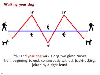
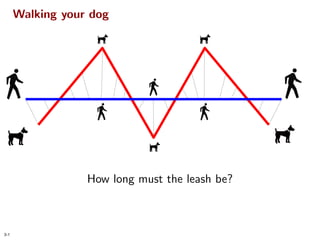
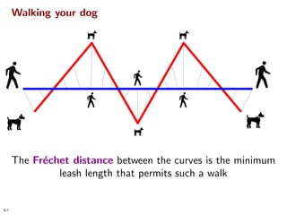
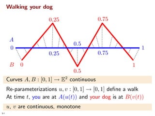
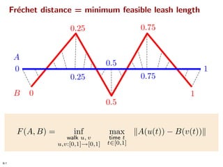
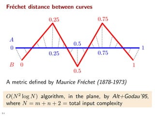
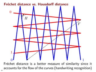
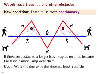
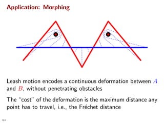
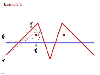
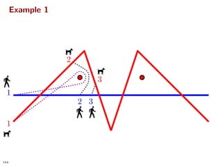
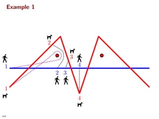
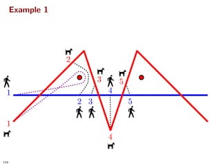
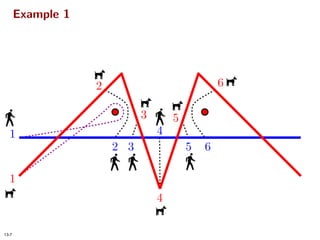
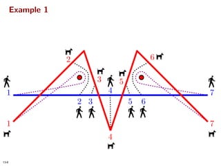
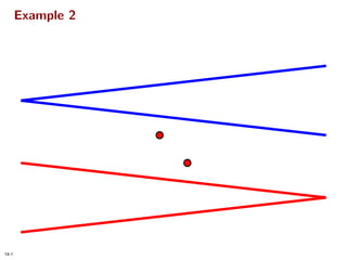
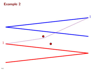
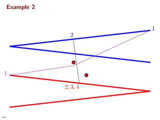
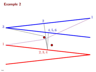
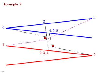
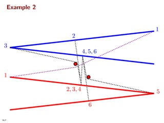
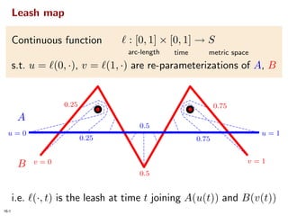
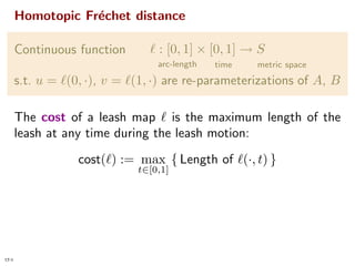
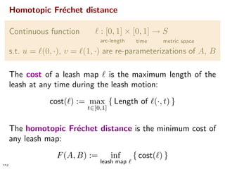
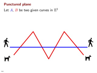
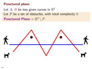
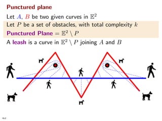
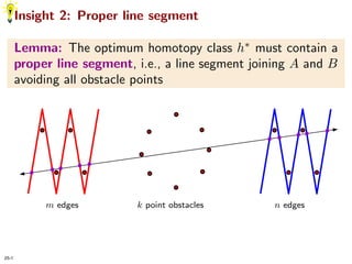
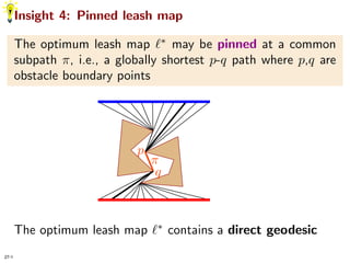
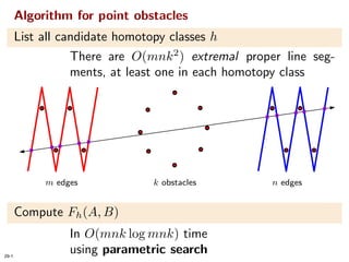
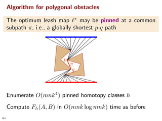
We define a generalization to arbitrary metric spaces of the classical Frechet distance between curves and give a polynomial-time algorithm to compute this so-called homotopic Frechet distance between polygonal curves in the plane with obstacles.
Rendering Technologies from Crysis 3 (GDC 2013)Tiago Sousa
This talk covers changes in CryENGINE 3 technology during 2012, with DX11 related topics such as moving to deferred rendering while maintaining backward compatibility on a multiplatform engine, massive vegetation rendering, MSAA support and how to deal with its common visual artifacts, among other topics.
Biography and career history of Bruno AmezcuaBruno Amezcua
Bruno Amezcua's entry into the film and visual arts world seemed predestined. His grandfather, a distinguished film editor from the 1950s through the 1970s, profoundly influenced him. This familial mentorship early on exposed him to the nuances of film production and a broad array of fine arts, igniting a lifelong passion for narrative creation. Over 15 years, Bruno has engaged in diverse projects showcasing his dedication to the arts.
Understanding the Mahadasha of Shukra (Venus): Effects and RemediesAstro Pathshala
The Mahadasha of Shukra (Venus) is one of the most significant periods in Vedic astrology. Shukra is known as the planet of love, beauty, wealth, and luxury. Its Mahadasha can bring about profound changes in an individual's life, both positive and negative, depending on its placement and condition in the natal chart.
What is Shukra Mahadasha?
Mahadasha is a planetary period in Vedic astrology that affects various aspects of an individual's life for a specific number of years. The Mahadasha of Shukra lasts for 20 years and is known to bring a period of significant transformation. Shukra is associated with pleasures, creativity, relationships, and material comforts. During its Mahadasha, these areas of life tend to get highlighted.
Care Instructions for Activewear & Swim Suits.pdfsundazesurf80
SunDaze Surf offers top swimwear tips: choose high-quality, UV-protective fabrics to shield your skin. Opt for secure fits that withstand waves and active movement. Bright colors enhance visibility, while adjustable straps ensure comfort. Prioritize styles with good support, like racerbacks or underwire tops, for active beach days. Always rinse swimwear after use to maintain fabric integrity.
The Fascinating World of Bats: Unveiling the Secrets of the Nightthomasard1122
The Fascinating World of Bats: Unveiling the Secrets of the Night
Bats, the mysterious creatures of the night, have long been a source of fascination and fear for humans. With their eerie squeaks and fluttering wings, they have captured our imagination and sparked our curiosity. Yet, beyond the myths and legends, bats are fascinating creatures that play a vital role in our ecosystem.
There are over 1,300 species of bats, ranging from the tiny Kitti's hog-nosed bat to the majestic flying foxes. These winged mammals are found in almost every corner of the globe, from the scorching deserts to the lush rainforests. Their diversity is a testament to their adaptability and resilience.
Bats are insectivores, feeding on a vast array of insects, from mosquitoes to beetles. A single bat can consume up to 1,200 insects in an hour, making them a crucial part of our pest control system. By preying on insects that damage crops, bats save the agricultural industry billions of dollars each year.
But bats are not just useful; they are also fascinating creatures. Their ability to fly in complete darkness, using echolocation to navigate and hunt, is a remarkable feat of evolution. They are also social animals, living in colonies and communicating with each other through a complex system of calls and body language.
Despite their importance, bats face numerous threats, from habitat destruction to climate change. Many species are endangered, and conservation efforts are necessary to protect these magnificent creatures.
In conclusion, bats are more than just creatures of the night; they are a vital part of our ecosystem, playing a crucial role in maintaining the balance of nature. By learning more about these fascinating animals, we can appreciate their importance and work to protect them for generations to come. So, let us embrace the beauty and mystery of bats, and celebrate their unique place in our world.
MRS PUNE 2024 - WINNER AMRUTHAA UTTAM JAGDHANEDK PAGEANT
Amruthaa Uttam Jagdhane, a stunning woman from Pune, has won the esteemed title of Mrs. India 2024, which is given out by the Dk Exhibition. Her journey to this prestigious accomplishment is a confirmation of her faithful assurance, extraordinary gifts, and profound commitment to enabling women.
At Affordable Garage Door Repair, we specialize in both residential and commercial garage door services, ensuring your property is secure and your doors are running smoothly.
Types of Garage Doors Explained: Energy Efficiency, Style, and More
Homotopic Frechet Distance Between Curves
1. Walking Your Dog in the
Woods in Polynomial Time
Shripad Thite
shripad@ Caltech.edu
´
Joint work with Erin Wolf Chambers, Eric Colin de Verdi`re,
e
Jeff Erickson, Sylvain Lazard, Francis Lazarus
at SoCG’08, invited to CGTA
1-1
2. Walking your dog
You and your dog walk along two given curves
from beginning to end, continuously without backtracking,
joined by a tight leash
2-1
4. Walking your dog
The Fr´chet distance between the curves is the minimum
e
leash length that permits such a walk
4-1
5. Walking your dog
0.75
0.25
A
0.5
0 1
0.75
0.25
0
B 1
0.5
Curves A, B : [0, 1] → E2 continuous
Re-parameterizations u, v : [0, 1] → [0, 1] define a walk
At time t, you are at A(u(t)) and your dog is at B(v(t))
u, v are continuous, monotone
5-1
6. Fr´chet distance = minimum feasible leash length
e
0.75
0.25
A
0.5
0 1
0.75
0.25
0
B 1
0.5
A(u(t)) − B(v(t))
F (A, B) = inf max
time t
walk u, v
t∈[0,1]
u,v:[0,1]→[0,1]
6-1
7. Fr´chet distance between curves
e
0.75
0.25
A
0.5
0 1
0.75
0.25
0
B 1
0.5
A metric defined by Maurice Fr´chet (1878-1973)
e
O(N 2 log N ) algorithm, in the plane, by Alt+Godau’95,
where N = m + n + 2 = total input complexity
7-1
8. Fr´chet distance vs. Hausdorff distance
e
0
H
F
1
0 1
Fr´chet distance is a better measure of similarity since it
e
accounts for the flow of the curves (handwriting recognition)
8-1
10. Woods have trees . . . and other obstacles
New condition: Leash must move continuously
If there are obstacles, a longer leash may be required because
the leash cannot jump over them
Goal: Walk the dog with the shortest leash possible
10-1
11. Homotopic Fr´chet distance
e
Dog-leash distance in a general metric space where the
leash must move continuously in the metric space
We give a polynomial-time algorithm to compute the ho-
motopic Fr´chet distance between two polygonal curves in
e
the plane with obstacles (= punctured plane)
11-1
12. Application: Morphing
Leash motion encodes a continuous deformation between A
and B, without penetrating obstacles
The “cost” of the deformation is the maximum distance any
point has to travel, i.e., the Fr´chet distance
e
12-1
30. Leash map
: [0, 1] × [0, 1] → S
Continuous function
arc-length time metric space
s.t. u = (0, ·), v = (1, ·) are re-parameterizations of A, B
0.25 0.75
A
0.5
u=0 u=1
0.25 0.75
v=1
v=0
B
0.5
i.e. (·, t) is the leash at time t joining A(u(t)) and B(v(t))
16-1
31. Homotopic Fr´chet distance
e
: [0, 1] × [0, 1] → S
Continuous function
arc-length time metric space
s.t. u = (0, ·), v = (1, ·) are re-parameterizations of A, B
The cost of a leash map is the maximum length of the
leash at any time during the leash motion:
cost( ) := max { Length of (·, t) }
t∈[0,1]
17-1
32. Homotopic Fr´chet distance
e
: [0, 1] × [0, 1] → S
Continuous function
arc-length time metric space
s.t. u = (0, ·), v = (1, ·) are re-parameterizations of A, B
The cost of a leash map is the maximum length of the
leash at any time during the leash motion:
cost( ) := max { Length of (·, t) }
t∈[0,1]
The homotopic Fr´chet distance is the minimum cost of
e
any leash map:
{ cost( ) }
F (A, B) := inf
leash map
17-2
35. Punctured plane
Let A, B be two given curves in E2
Let P be a set of obstacles, with total complexity k
Punctured Plane = E2 P
19-2
36. Punctured plane
Let A, B be two given curves in E2
Let P be a set of obstacles, with total complexity k
Punctured Plane = E2 P
A leash is a curve in E2 P joining A and B
19-3
37. Punctured plane
Let A, B be two given curves in E2
Let P be a set of obstacles, with total complexity k
Punctured Plane = E2 P
A leash is a curve in E2 P joining A and B
Leash map : [0, 1] × [0, 1] → E2 P must be continuous;
so, the leash cannot jump over obstacles
19-4
38. Relative homotopy
Two leashes are relatively homotopic if one can be con-
tinuously transformed into the other in the punctured plane
while keeping their endpoints on the respective curves
20-1
39. Relative homotopy
Two leashes are relatively homotopic if one can be con-
tinuously transformed into the other in the punctured plane
while keeping their endpoints on the respective curves
Functions α, β : X → Y are (freely) homotopic if there is a continuous function
h : X × [0, 1] → Y such that h(·, 0) = α(·) and h(·, 1) = β(·)
20-2
40. Relative homotopy class
Every leash map h describes a set of leashes belonging to
some relative homotopy class h
21-1
42. Homotopic Fr´chet distance redux
e
Let h be a relative homotopy class
Let be a leash map in homotopy class h
h
22-2
43. Homotopic Fr´chet distance redux
e
Let h be a relative homotopy class
Let be a leash map in homotopy class h
h
{ cost( h ) }
Let Fh (A, B) := inf h
22-3
44. Homotopic Fr´chet distance redux
e
Let h be a relative homotopy class
Let be a leash map in homotopy class h
h
{ cost( h ) }
Let Fh (A, B) := inf h
Homotopic Fr´chet distance
e
F (A, B) := min{Fh (A, B)}
h
22-4
46. Insight 1: Geodesic leashes
Lemma: There exists an optimum leash map such that the
leash at every time is the shortest path in its homotopy class
24-1
47. Insight 1: Geodesic leashes
Lemma: There exists an optimum leash map such that the
leash at every time is the shortest path in its homotopy class
Hence, w.l.o.g., ∗ (·, t) is the (unique) geodesic in homotopy
h
class h between its endpoints
24-2
48. Insight 1: Geodesic leashes
Lemma: There exists an optimum leash map such that the
leash at every time is the shortest path in its homotopy class
Hence, w.l.o.g., ∗ (·, t) is the (unique) geodesic in homotopy
h
class h between its endpoints
Fact: The geodesic between a ∈ A and b ∈ B moves
continuously as a,b move continuously along their respective
curves
24-3
49. Insight 1: Geodesic leashes
Lemma: There exists an optimum leash map such that the
leash at every time is the shortest path in its homotopy class
Hence, w.l.o.g., ∗ (·, t) is the (unique) geodesic in homotopy
h
class h between its endpoints
Fact: The geodesic between a ∈ A and b ∈ B moves
continuously as a,b move continuously along their respective
curves
but . . . there are infinitely many geodesics with the same
endpoints, one in each of infinitely many homotopy classes
24-4
50. Insight 2: Proper line segment
Lemma: The optimum homotopy class h∗ must contain a
proper line segment, i.e., a line segment joining A and B
avoiding all obstacle points
m edges k point obstacles n edges
25-1
51. Insight 3: Minimal homotopy classes
A homotopy class is minimal if it does not bend around
obstacles unnecessarily
Lemma: There exists an optimum homotopy class that is
minimal
Lemma: Every minimal homotopy class contains a proper
line segment
Here onwards, we speak only of minimal homotopy classes
26-1
52. Insight 4: Pinned leash map
The optimum leash map ∗ may be pinned at a common
subpath π, i.e., a globally shortest p-q path where p,q are
obstacle boundary points
p
π
q
∗
The optimum leash map contains a direct geodesic
27-1
54. Algorithm for point obstacles
List all candidate homotopy classes h
There are O(mnk 2 ) extremal proper line seg-
ments, at least one in each homotopy class
m edges k obstacles n edges
Compute Fh (A, B)
In O(mnk log mnk) time
using parametric search
29-1
55. Algorithm for polygonal obstacles
The optimum leash map ∗ may be pinned at a common
subpath π, i.e., a globally shortest p-q path
p
π
q
Enumerate O(mnk 4 ) pinned homotopy classes h
Compute Fh (A, B) in O(mnk log mnk) time as before
30-1
57. We defined the homotopic Fr´chet distance between two
e
curves in a general metric space
the most natural generalization of Fr´chet distance
e
to arbitrary metric spaces
We gave a polynomial-time algorithm to compute the homo-
topic Fr´chet distance between two polygonal curves A,B
e
in the plane with point or polygonal obstacles
the punctured plane is the first metric space
that we consider
32-1
58. Open problem: On a convex polyhedron
Leash is not always a geodesic!
e.g., leash must have enough slack to cross over a vertex
(a ‘mountain’)
Challenge: Characterize an optimum leash map
33-1
62. Computing Fh
Decision problem: Given a real d ≥ 0, is Fh (A, B) ≤ d?
37-1
63. Computing Fh
Decision problem: Given a real d ≥ 0, is Fh (A, B) ≤ d?
Observation: There are polynomially many critical values
of d at which the answer may change from ‘no’ to ‘yes’
d1 ≤ d2 ≤ . . . ≤ di−1 ≤ d∗ ≤ di+1 ≤ di+2 ≤ . . .
37-2
64. Computing Fh
Decision problem: Given a real d ≥ 0, is Fh (A, B) ≤ d?
Observation: There are polynomially many critical values
of d at which the answer may change from ‘no’ to ‘yes’
d1 ≤ d2 ≤ . . . ≤ di−1 ≤ d∗ ≤ di+1 ≤ di+2 ≤ . . .
37-3
65. Computing Fh
Decision problem: Given a real d ≥ 0, is Fh (A, B) ≤ d?
Observation: There are polynomially many critical values
of d at which the answer may change from ‘no’ to ‘yes’
d1 ≤ d2 ≤ . . . ≤ di−1 ≤ d∗ ≤ di+1 ≤ di+2 ≤ . . .
Fh (A, B)
Goal: Find the smallest critical value d for which the answer
above is ‘yes’
37-4
66. Is Fh ≤ d?
i + 1, j + 1
|P | changes
|P | changes
i, j
http://www.cim.mcgill.ca/∼stephane/cs507/Project.html, St´phane Pelletier, 2002
e
Is there a monotone path from (0, 0) to (m, n) in free space?
Key lemma: Free space within each cell Cij is convex
i.e., leash length is a convex function along any monotone path through Cij
(think hourglasses)
38-1
67. Computing free space
i + 1, j i + 1, j + 1
i, j i, j + 1
Given the shortest path between ai and bj , compute:
(1) the interval b ∈ [bj , bj+1 ] such that dist(ai , b) ≤ d
(2) the interval a ∈ [ai , ai+1 ] such that dist(bj , a) ≤ d
(3) shortest paths (ai , bj+1 ), (ai+1 , bj ), and (ai+1 , bj+1 )
39-1
68. Funnels
Shortest paths from ai to
[bj , bj+1 ] define a funnel∗
∗ in the universal cover
40-1
69. Funnels
Shortest paths from ai to bj+1
b
[bj , bj+1 ] define a funnel∗
∗ in the universal cover
bj
Leash evolves like a deque apex
as its endpoints sweep
tail
ai
40-2
70. Funnels
Shortest paths from ai to bj+1
b
[bj , bj+1 ] define a funnel∗
∗ in the universal cover
bj
Leash evolves like a deque apex
as its endpoints sweep
tail
ai
In O(k log k) time, build a funnel data structure of size
O(k), using a deque, such that each free interval can be
computed in O(log k) time
40-3
71. Computing Fh
Decision algorithm: Given a real d ≥ 0, is Fh (A, B) ≤ d?
. . . in O(mn log k) time
41-1
72. Computing Fh
Decision algorithm: Given a real d ≥ 0, is Fh (A, B) ≤ d?
. . . in O(mn log k) time
Observation: There are polynomially many critical values
of d at which the answer may change from ‘no’ to ‘yes’
d1 ≤ d2 ≤ . . . ≤ di−1 ≤ d∗ ≤ di+1 ≤ di+2 ≤ . . .
41-2
73. Computing Fh
Decision algorithm: Given a real d ≥ 0, is Fh (A, B) ≤ d?
. . . in O(mn log k) time
Observation: There are polynomially many critical values
of d at which the answer may change from ‘no’ to ‘yes’
d1 ≤ d2 ≤ . . . ≤ di−1 ≤ d∗ ≤ di+1 ≤ di+2 ≤ . . .
41-3
74. Computing Fh
Decision algorithm: Given a real d ≥ 0, is Fh (A, B) ≤ d?
. . . in O(mn log k) time
Observation: There are polynomially many critical values
of d at which the answer may change from ‘no’ to ‘yes’
d1 ≤ d2 ≤ . . . ≤ di−1 ≤ d∗ ≤ di+1 ≤ di+2 ≤ . . .
Fh (A, B)
Goal: Find the smallest critical value d for which the answer
above is ‘yes’
41-4
75. Parametric search [Megiddo ’83]
Let As be an algorithm to decide, given a critical value di ,
whether Fh (A, B) ≤ di , with running time O(Ts )
d1 ≤ d2 ≤ . . . ≤ di−1 ≤ d∗ ≤ . . . ≤ dj ≤ . . .
42-1
76. Parametric search [Megiddo ’83]
Let As be an algorithm to decide, given a critical value di ,
whether Fh (A, B) ≤ di , with running time O(Ts )
d1 ≤ d2 ≤ . . . ≤ di−1 ≤ d∗ ≤ . . . ≤ dj ≤ . . .
We simulate As on input d∗ , with d∗ as a symbolic variable
42-2
77. Parametric search [Megiddo ’83]
Let As be an algorithm to decide, given a critical value di ,
whether Fh (A, B) ≤ di , with running time O(Ts )
d1 ≤ d2 ≤ . . . ≤ di−1 ≤ d∗ ≤ . . . ≤ dj ≤ . . .
We simulate As on input d∗ , with d∗ as a symbolic variable
The control flow of As depends on comparisons of the form
d∗ ≤ dj where dj is a critical value
Each dj is a distance, i.e., a quadratic function of input coordinates.
42-3
78. Parametric search [Megiddo ’83]
Let As be an algorithm to decide, given a critical value di ,
whether Fh (A, B) ≤ di , with running time O(Ts )
d1 ≤ d2 ≤ . . . ≤ di−1 ≤ d∗ ≤ . . . ≤ dj ≤ . . .
We simulate As on input d∗ , with d∗ as a symbolic variable
The control flow of As depends on comparisons of the form
d∗ ≤ dj where dj is a critical value
Each dj is a distance, i.e., a quadratic function of input coordinates.
d∗ ≤ dj ? Run As on input dj , in O(Ts ) time
42-4
79. Parametric search [Megiddo ’83]
Let As be an algorithm to decide, given a critical value di ,
whether Fh (A, B) ≤ di , with running time O(Ts )
d1 ≤ d2 ≤ . . . ≤ di−1 ≤ d∗ ≤ . . . ≤ dj ≤ . . .
We simulate As on input d∗ , with d∗ as a symbolic variable
The control flow of As depends on comparisons of the form
d∗ ≤ dj where dj is a critical value
Each dj is a distance, i.e., a quadratic function of input coordinates.
d∗ ≤ dj ? Run As on input dj , in O(Ts ) time
2
Total running time = O(Ts )
42-5
80. Parametric search on steroids [Megiddo ’83]
Let Ap be a parallel algorithm to decide, given di , whether
Fh (A, B) ≤ di , with parallel running time O(Tp ) on q pro-
cessors
d1 ≤ d2 ≤ . . . ≤ di−1 ≤ d∗ ≤ . . . ≤ dj ≤ . . .
43-1
81. Parametric search on steroids [Megiddo ’83]
Let Ap be a parallel algorithm to decide, given di , whether
Fh (A, B) ≤ di , with parallel running time O(Tp ) on q pro-
cessors
d1 ≤ d2 ≤ . . . ≤ di−1 ≤ d∗ ≤ . . . ≤ dj ≤ . . .
We simulate Ap sequentially on input d∗ , with d∗ as a
symbolic variable
43-2
82. Parametric search on steroids [Megiddo ’83]
Let Ap be a parallel algorithm to decide, given di , whether
Fh (A, B) ≤ di , with parallel running time O(Tp ) on q pro-
cessors
d1 ≤ d2 ≤ . . . ≤ di−1 ≤ d∗ ≤ . . . ≤ dj ≤ . . .
We simulate Ap sequentially on input d∗ , with d∗ as a
symbolic variable
The control flow of Ap depends on comparisons of the form
d∗ ≤ dj where dj is a critical value
43-3
83. Parametric search on steroids [Megiddo ’83]
Let Ap be a parallel algorithm to decide, given di , whether
Fh (A, B) ≤ di , with parallel running time O(Tp ) on q pro-
cessors
d1 ≤ d2 ≤ . . . ≤ di−1 ≤ d∗ ≤ . . . ≤ dj ≤ . . .
We simulate Ap sequentially on input d∗ , with d∗ as a
symbolic variable
The control flow of Ap depends on comparisons of the form
d∗ ≤ dj where dj is a critical value
In each parallel stage, do binary search on O(q) values dj
43-4
84. Parametric search on steroids [Megiddo ’83]
Let Ap be a parallel algorithm to decide, given di , whether
Fh (A, B) ≤ di , with parallel running time O(Tp ) on q pro-
cessors
d1 ≤ d2 ≤ . . . ≤ di−1 ≤ d∗ ≤ . . . ≤ dj ≤ . . .
We simulate Ap sequentially on input d∗ , with d∗ as a
symbolic variable
The control flow of Ap depends on comparisons of the form
d∗ ≤ dj where dj is a critical value
In each parallel stage, do binary search on O(q) values dj
Total running time = O(Ts Tp log q + qTp ) 2
better than O(Ts )
43-5
85. How we use parametric search
Let Ap be a parallel sorting algorithm
(e.g., Cole’s parallel merge sort)
44-1
86. How we use parametric search
Let Ap be a parallel sorting algorithm
(e.g., Cole’s parallel merge sort)
We use Ap to sort O(mn) critical distances with parallel
running time O(log mn)
We simulate Ap sequentially on input d∗ , with d∗ as a
symbolic variable
44-2
87. How we use parametric search
Let Ap be a parallel sorting algorithm
(e.g., Cole’s parallel merge sort)
We use Ap to sort O(mn) critical distances with parallel
running time O(log mn)
We simulate Ap sequentially on input d∗ , with d∗ as a
symbolic variable
The control flow of Ap depends on comparisons of the form
d∗ ≤ dj where dj is a critical value
44-3
88. How we use parametric search
Let Ap be a parallel sorting algorithm
(e.g., Cole’s parallel merge sort)
We use Ap to sort O(mn) critical distances with parallel
running time O(log mn)
We simulate Ap sequentially on input d∗ , with d∗ as a
symbolic variable
The control flow of Ap depends on comparisons of the form
d∗ ≤ dj where dj is a critical value
To simulate each parallel stage, we resolve all O(mn) com-
parisons d∗ ≤ dj by computing O(mnk) critical intervals
and locating each dj in some interval
44-4
89. How we use parametric search
Let Ap be a parallel sorting algorithm
(e.g., Cole’s parallel merge sort)
We use Ap to sort O(mn) critical distances with parallel
running time O(log mn)
We simulate Ap sequentially on input d∗ , with d∗ as a
symbolic variable
The control flow of Ap depends on comparisons of the form
d∗ ≤ dj where dj is a critical value
To simulate each parallel stage, we resolve all O(mn) com-
parisons d∗ ≤ dj by computing O(mnk) critical intervals
and locating each dj in some interval
Total running time = O(N 3 log N )
44-5