The document discusses pro forma financial statements and forecasting additional funds needed (AFN). It provides examples of forecasting a company's income statement, balance sheet, and AFN for the year 2005 based on 2004 actuals and assumptions. The AFN is calculated as $187.2 million, which will be raised as $93.6 million in notes payable and $93.6 million in long-term debt. Differences from the equation method AFN are due to the pro forma method allowing flexible growth rates. Excess capacity and economies of scale can impact AFN forecasts.

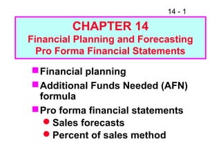
1. 14 - 1
CHAPTER 14
Financial Planning and Forecasting
Pro Forma Financial Statements
Financial planning
Additional Funds Needed (AFN)
formula
Pro forma financial statements
Sales forecasts
Percent of sales method

2. 14 - 2
Financial Planning and
Pro Forma Statements
Three important uses:
Forecast the amount of external
financing that will be required
Evaluate the impact that changes
in the operating plan have on the
value of the firm
Set appropriate targets for
compensation plans

3. 14 - 3
Steps in Financial Forecasting
Forecast sales
Project the assets needed to support
sales
Project internally generated funds
Project outside funds needed
Decide how to raise funds
See effects of plan on ratios and
stock price

4. 14 - 4
2004 Balance Sheet
(Millions of $)
Cash & sec. $ 20 Accts. pay. &
accruals $ 100
Accounts rec. 240 Notes payable 100
Inventories 240 Total CL $ 200
Total CA $ 500 L-T debt 100
Common stk 500
Net fixed
assets
Retained
earnings 200
Total assets $1,000 Total claims $1,000
500

5. 14 - 5
2004 Income Statement
(Millions of $)
Sales $2,000.00
Less: COGS (60%) 1,200.00
SGA costs 700.00
EBIT $ 100.00
Interest 10.00
EBT $ 90.00
Taxes (40%) 36.00
Net income $ 54.00
Dividends (40%) $21.60
Add’n to RE $32.40

6. 14 - 6
AFN (Additional Funds Needed):
Key Assumptions
Operating at full capacity in 2004.
Each type of asset grows proportionally
with sales.
Payables and accruals grow proportionally
with sales.
2004 profit margin ($54/$2,000 = 2.70%)
and payout (40%) will be maintained.
Sales are expected to increase by $500
million.

7. 14 - 7
Definitions of Variables in AFN
A*/S0: assets required to support
sales; called capital intensity ratio.
∆S: increase in sales.
L*/S0: spontaneous liabilities ratio
M: profit margin (Net income/sales)
RR: retention ratio; percent of net
income not paid as dividend.

8. 14 - 8
Assets
Sales0
1,000
2,000
1,250
2,500
A*/S0 = $1,000/$2,000 = 0.5 = $1,250/$2,500.
∆ Assets =
(A*/S0)∆Sales
= 0.5($500)
= $250.
Assets = 0.5 sales

9. 14 - 9
Assets must increase by $250 million.
What is the AFN, based on the AFN
equation?
AFN = (A*/S0)∆S - (L*/S0)∆S - M(S1)(RR)
= ($1,000/$2,000)($500)
- ($100/$2,000)($500)
- 0.0270($2,500)(1 - 0.4)
= $184.5 million.

10. 14 - 10
How would increases in these items
affect the AFN?
Higher sales:
Increases asset requirements,
increases AFN.
Higher dividend payout ratio:
Reduces funds available
internally, increases AFN.
(More…)

11. 14 - 11
Higher profit margin:
Increases funds available
internally, decreases AFN.
Higher capital intensity ratio, A*/S0:
Increases asset requirements,
increases AFN.
Pay suppliers sooner:
Decreases spontaneous liabilities,
increases AFN.

12. 14 - 12
Projecting Pro Forma Statements with
the Percent of Sales Method
Project sales based on forecasted
growth rate in sales
Forecast some items as a percent
of the forecasted sales
Costs
Cash
Accounts receivable (More...)

13. 14 - 13
Items as percent of sales (Continued...)
Inventories
Net fixed assets
Accounts payable and accruals
Choose other items
Debt
Dividend policy (which determines
retained earnings)
Common stock

14. 14 - 14
Sources of Financing Needed to
Support Asset Requirements
Given the previous assumptions and
choices, we can estimate:
Required assets to support sales
Specified sources of financing
Additional funds needed (AFN) is:
Required assets minus specified
sources of financing

15. 14 - 15
Implications of AFN
If AFN is positive, then you must
secure additional financing.
If AFN is negative, then you have
more financing than is needed.
Pay off debt.
Buy back stock.
Buy short-term investments.

16. 14 - 16
How to Forecast Interest Expense
Interest expense is actually based on
the daily balance of debt during the
year.
There are three ways to approximate
interest expense. Base it on:
Debt at end of year
Debt at beginning of year
Average of beginning and ending
debt
More…

17. 14 - 17
Basing Interest Expense
on Debt at End of Year
Will over-estimate interest expense if
debt is added throughout the year
instead of all on January 1.
Causes circularity called financial
feedback: more debt causes more
interest, which reduces net income,
which reduces retained earnings,
which causes more debt, etc.
More…

18. 14 - 18
Basing Interest Expense
on Debt at Beginning of Year
Will under-estimate interest expense
if debt is added throughout the year
instead of all on December 31.
But doesn’t cause problem of
circularity.
More…

19. 14 - 19
Basing Interest Expense on Average of
Beginning and Ending Debt
Will accurately estimate the interest
payments if debt is added smoothly
throughout the year.
But has problem of circularity.
More…

20. 14 - 20
A Solution that Balances Accuracy and
Complexity
Base interest expense on beginning
debt, but use a slightly higher
interest rate.
Easy to implement
Reasonably accurate
See Ch 14 Mini Case Feedback.xls
for an example basing interest
expense on average debt.

21. 14 - 21
Percent of Sales: Inputs
COGS/Sales 60% 60%
SGA/Sales 35% 35%
Cash/Sales 1% 1%
Acct. rec./Sales 12% 12%
Inv./Sales 12% 12%
Net FA/Sales 25% 25%
AP & accr./Sales 5% 5%
2004 2005
Actual Proj.

22. 14 - 22
Other Inputs
Percent growth in sales 25%
Growth factor in sales (g) 1.25
Interest rate on debt 10%
Tax rate 40%
Dividend payout rate 40%

23. 14 - 23
2005 Forecasted Income Statement
2004 Factor
2005
1st Pass
Sales $2,000 g=1.25 $2,500.0
Less: COGS Pct=60% 1,500.0
SGA Pct=35% 875.0
EBIT $125.0
Interest 0.1(Debt04) 20.0
EBT $105.0
Taxes (40%) 42.0
Net. income $63.0
Div. (40%) $25.2
Add. to RE $37.8

24. 14 - 24
2005 Balance Sheet (Assets)
Forecasted assets are a percent of forecasted sales.
Factor 2005
Cas
h
Pct= 1% $25.0
Accts. rec. Pct=12% 300.0
Pct=12% 300.0
Total
CA
$625.0
Net FA Pct=25% 625.0
Total assets $1,250.0
2005 Sales = $2,500
Inventories

25. 14 - 25
2005 Preliminary Balance Sheet (Claims)
*From forecasted income statement.
2004 Factor Without AFN
AP/accruals Pct=5% $125.0
Notes payable 100 100.0
Total CL $225.0
L-T debt 100 100.0
Common stk. 500 500.0
Ret. earnings 200 +37.8* 237.8
Total claims $1,062.8
2005
2005 Sales = $2,500

26. 14 - 26
Required assets = $1,250.0
Specified sources of fin. = $1,062.8
Forecast AFN = $ 187.2
What are the additional funds
needed (AFN)?
NWC must have the assets to make
forecasted sales, and so it needs an
equal amount of financing. So, we must
secure another $187.2 of financing.

27. 14 - 27
Assumptions about How AFN Will
Be Raised
No new common stock will be
issued.
Any external funds needed will be
raised as debt, 50% notes payable,
and 50% L-T debt.

28. 14 - 28
How will the AFN be financed?
Additional notes payable =
0.5 ($187.2) = $93.6.
Additional L-T debt =
0.5 ($187.2) = $93.6.

29. 14 - 29
2005 Balance Sheet (Claims)
w/o AFN AFN With AFN
AP/accruals $ 125.0 $ 125.0
Notes payable 100.0 +93.6 193.6
Total CL $ 225.0 $ 318.6
L-T debt 100.0 +93.6 193.6
Common stk. 500.0 500.0
Ret. earnings 237.8 237.8
Total claims $1,071.0 $1,250.0

30. 14 - 30
Equation method assumes a
constant profit margin.
Pro forma method is more flexible.
More important, it allows different
items to grow at different rates.
Equation AFN = $184.5
vs.
Pro Forma AFN = $187.2.
Why are they different?

31. 14 - 31
Forecasted Ratios
2004 2005(E) Industry
Profit Margin 2.70% 2.52% 4.00%
ROE 7.71% 8.54% 15.60%
DSO (days) 43.80 43.80 32.00
Inv. turnover 8.33x 8.33x 11.00x
FA turnover 4.00x 4.00x 5.00x
Debt ratio 30.00% 40.98% 36.00%
TIE 10.00x 6.25x 9.40x
Current ratio 2.50x 1.96x 3.00x

32. 14 - 32
What are the forecasted
free cash flow and ROIC?
2004 2005(E)
Net operating WC $400 $500
(CA - AP & accruals)
Total operating capital $900 $1,125
(Net op. WC + net FA)
NOPAT (EBITx(1-T)) $60 $75
Less Inv. in op. capital $225
Free cash flow -$150
ROIC (NOPAT/Capital) 6.7%

33. 14 - 33
Proposed Improvements
DSO (days) 43.80 32.00
Accts. rec./Sales 12.00% 8.77%
Inventory turnover 8.33x 11.00x
Inventory/Sales 12.00% 9.09%
SGA/Sales 35.00% 33.00%
Before After

34. 14 - 34
Impact of Improvements
(see Ch 14 Mini Case.xls for details)
AFN $187.2 $15.7
Free cash flow -$150.0 $33.5
ROIC (NOPAT/Capital) 6.7% 10.8%
ROE 7.7% 12.3%
Before After

35. 14 - 35
Suppose in 2004 fixed assets had been
operated at only 75% of capacity.
With the existing fixed assets, sales
could be $2,667. Since sales are
forecasted at only $2,500, no new
fixed assets are needed.
Capacity sales =
Actual sales
% of capacity
= = $2,667.
$2,000
0.75

36. 14 - 36
How would the excess capacity
situation affect the 2005 AFN?
The previously projected increase in
fixed assets was $125.
Since no new fixed assets will be
needed, AFN will fall by $125, to
$187.2 - $125 = $62.2.

37. 14 - 37
Assets
Sales
0
1,100
1,000
2,000 2,500
Declining A/S Ratio
$1,000/$2,000 = 0.5; $1,100/$2,500 = 0.44. Declining
ratio shows economies of scale. Going from S = $0
to S = $2,000 requires $1,000 of assets. Next $500 of
sales requires only $100 of assets.
Base
Stock
}
Economies of Scale

38. 14 - 38
Assets
Sales
1,000 2,000500
A/S changes if assets are lumpy. Generally will have
excess capacity, but eventually a small ∆S leads to a
large ∆A.
500
1,000
1,500
Lumpy Assets

39. 14 - 39
Summary: How different factors affect
the AFN
forecast.
Excess capacity: lowers AFN.
Economies of scale: leads to less-than-
proportional asset increases.
Lumpy assets: leads to large periodic
AFN requirements, recurring excess
capacity.