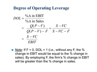
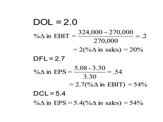
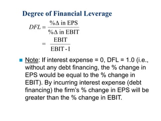
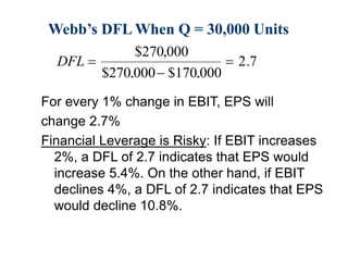
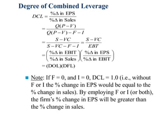
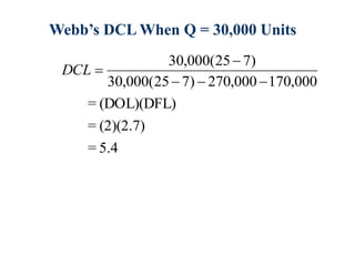
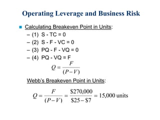
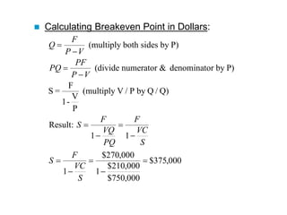
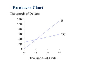
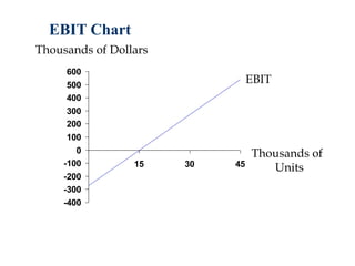
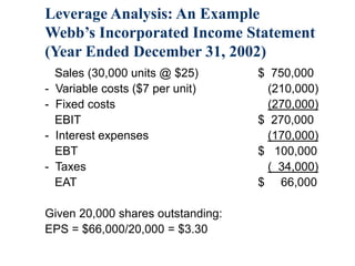
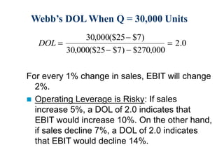
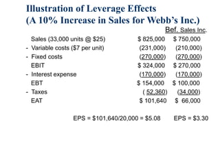
This document discusses operating leverage, financial leverage, and combined leverage. It defines key terms like operating leverage, financial leverage, fixed costs, variable costs, and provides examples and calculations for: - Degree of operating leverage (DOL) - Degree of financial leverage (DFL) - Degree of combined leverage (DCL) - Breakeven analysis and charts - An example calculation using financial statements for Webb's Inc. to illustrate the effects of a 10% increase in sales on earnings, operating income, and earnings per share through the application of leverage.

1. Operating and Financial Leverage
(Chapter 5)
 Business and Financial Risk
 Employing Leverage
 Leverage and the Income Statement
 Operating Leverage and
Business Risk
 Breakeven Analysis
 Degree of Operating Leverage
 Degree of Financial Leverage
 Degree of Combined Leverage
 Illustration of Leverage Effects

2. Business and Financial Risk
 Business Risk - Uncertainty inherent in the
firm’s operations if it used no debt.
 Major Factors Affecting Business Risk:
– Total sales variability
– Total fixed operating expenses
 Financial Risk – Additional risk incurred
through the use of debt financing.

3. Employing Leverage
 Leverage:
– Use of “fixed cost” items in the process of
magnifying earnings.
 Operating Leverage:
– Use of “fixed operating costs” in the process of
magnifying operating income (EBIT)
 Financial Leverage:
– Use of “fixed financial costs” (e.g., debt and
preferred stock financing) in the process of
magnifying earnings per share EPS. Our
discussion focuses on the use of debt financing.

4. Leverage and the Income Statement
Sales
- Fixed costs
- Variable costs
EBIT
- Interest
EBT
- Taxes
EAT
Note: EPS = EAT/(# shares) [assuming no pfd. stock]
Operating Leverage
Financial Leverage
Total
Leverage

5. Leverage Analysis: An Example
Webb’s Incorporated Income Statement
(Year Ended December 31, 2002)
Sales (30,000 units @ $25) $ 750,000
- Variable costs ($7 per unit) (210,000)
- Fixed costs (270,000)
EBIT $ 270,000
- Interest expenses (170,000)
EBT $ 100,000
- Taxes ( 34,000)
EAT $ 66,000
Given 20,000 shares outstanding:
EPS = $66,000/20,000 = $3.30

6. Key to Symbols Used in
the Following Analyses
Note: The symbols used in the notes differ
somewhat from the symbols used in the text.
 P = price per unit
 Q = sales in units
 V = variable cost per unit
 F = fixed costs
 VC = total variable costs
 TC = F + VC = total costs
 S = PQ = sales dollars
 EBIT = S - TC

7. Operating Leverage and Business Risk
 Calculating Breakeven Point in Units:
– (1) S - TC = 0
– (2) S - F - VC = 0
– (3) PQ - F - VQ = 0
– (4) PQ - VQ = F
Webb’s Breakeven Point in Units:
Q
F
P V


( )
Q
F
P V





( )
$270,
$25 $7
,
000
15 000 units

8.  Calculating Breakeven Point in Dollars:
Q
F
P V
PQ
PF
P V
S
F
VQ
PQ
F
VC
S
S
F
VC
S













(multiply both sides by P)
(divide numerator & denominator by P)
S =
F
1-
V
P
(multiply V / P by Q / Q)
Result:
1 1
1
000
1
000
000
000
$270,
$210,
$750,
$375,

9. Breakeven Chart
0
200
400
600
800
1000
1200
0 15 30 45
Thousands of Dollars
Thousands of Units
S
TC

10. EBIT Chart
-400
-300
-200
-100
0
100
200
300
400
500
600
15 30 45
Thousands of Dollars
Thousands of
Units
EBIT

11. Degree of Operating Leverage
 Note: If F = 0, DOL = 1 (i.e., without any F, the %
change in EBIT would be equal to the % change in
sales). By employing F, the firm’s % change in EBIT
will be greater than the % change in sales.
DOL
Q P V
Q P V F
S VC
S VC F
S VC
EBIT


 


 

% in EBIT
in Sales
=
=


%
( )
( )

12. Webb’s DOL When Q = 30,000 Units
For every 1% change in sales, EBIT will change
2%.
 Operating Leverage is Risky: If sales
increase 5%, a DOL of 2.0 indicates that
EBIT would increase 10%. On the other hand,
if sales decline 7%, a DOL of 2.0 indicates
that EBIT would decline 14%.
DOL 

 

30 000
30 000 000
2 0
, ($25 $7)
, ($25 $7) $270,
.

13. Degree of Financial Leverage
 Note: If interest expense = 0, DFL = 1.0 (i.e.,
without any debt financing, the % change in
EPS would be equal to the % change in
EBIT). By incurring interest expense (debt
financing) the firm’s % change in EPS will be
greater than the % change in EBIT.
DFL 
%
%


in EPS
in EBIT
=
EBIT
EBIT -I

14. Webb’s DFL When Q = 30,000 Units
For every 1% change in EBIT, EPS will
change 2.7%
Financial Leverage is Risky: If EBIT increases
2%, a DFL of 2.7 indicates that EPS would
increase 5.4%. On the other hand, if EBIT
declines 4%, a DFL of 2.7 indicates that EPS
would decline 10.8%.
DFL 


$270,
$270, $170,
.
000
000 000
2 7

15. Degree of Combined Leverage
 Note: If F = 0, and I = 0, DCL = 1.0 (i.e., without
F or I the % change in EPS would be equal to the
% change in sales). By employing F or I (or both),
the firm’s % change in EPS will be greater than
the % change in sales.
(DOL)(DFL)
=
EBIT
in
%
EPS
in
%
Sales
in
%
EBIT
in
%
=
=
)
(
)
(
=
Sales
in
%
EPS
in
%





























EBT
VC
S
I
F
VC
S
VC
S
I
F
V
P
Q
V
P
Q
DCL

16. Webb’s DCL When Q = 30,000 Units
5.4
=
(2)(2.7)
=
(DOL)(DFL)
=
000
,
170
000
,
270
)
7
25
(
000
,
30
)
7
25
(
000
,
30





DCL

17. Illustration of Leverage Effects
(A 10% Increase in Sales for Webb’s Inc.)
Bef. Sales Inc.
Sales (33,000 units @ $25) $ 825,000 $ 750,000
- Variable costs ($7 per unit) (231,000) (210,000)
- Fixed costs (270,000) (270,000)
EBIT $ 324,000 $ 270,000
- Interest expense (170,000) (170,000)
EBT $ 154,000 $ 100,000
- Taxes ( 52,360) (34,000)
EAT $ 101,640 $ 66,000
EPS = $101,640/20,000 = $5.08 EPS = $3.30

18. 54%
=
sales)
in
5.4(%
=
EPS
in
%
54%
=
EBIT)
in
2.7(%
=
.54
=
30
.
3
3.30
-
5.08
=
EPS
in
%
20%
=
sales)
in
2(%
=
2
.
000
,
270
000
,
270
000
,
324
=
EBIT
in
%








5.4
=
DCL
2.7
=
DFL
2.0
=
DOL