
![30
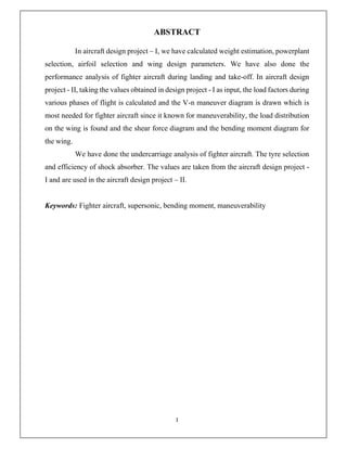
Volume of the fuel tank
Vfuel = Area * t
= {Area rectangle + 2(Area triangle)}*t
= {(h*l2) +2[ h
( )
]}*t
={(h*l2) + [ h (l1 − l2)]}*t
={(h*(
( . )
) Croot ) + [ h (
( . ) ( . )
)]}*t
={((
( . )
) Croot ) +[
(Croot b−0.2−b−h−0.2 )
b
]}h*t
={(b − h − 0.2)+[0.5(b-0.2-b+h+0.2)]} h*t
= {(b − h − 0.2)+0.5h} h*t
Vfuel =
root
h ∗ t (b − − 0.2)
Density of fuel, 𝜌𝑓𝑢𝑒𝑙 =
Vfuel = (
𝑚
ρ
) fuel
Where,
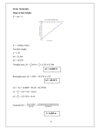
Mass of fuel, m = 932.79 kg
Density of fuel, 𝜌 = 801 kg/m
Vfuel =
.
=1.16 m
Vfuel = 1.16 𝐦𝟑
Solving h,
Vfuel =
root
h ∗ t (b − − 0.2)
Where,
Vfuel = 1.16 m
Half span, b = 5.04 m
Croot = 3.6 m](https://image.slidesharecdn.com/finalfighteraircraftdesignadp2-211125180150/85/Final-fighter-aircraft-design-adp-2-39-320.jpg)

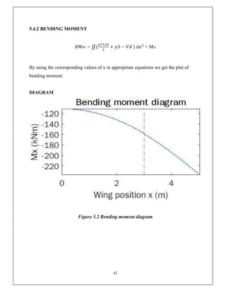
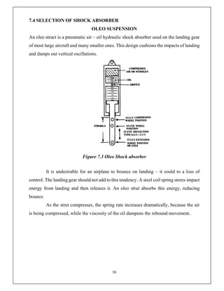

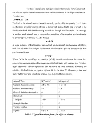
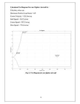
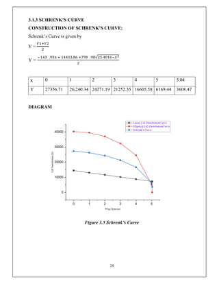
This document discusses the V-n diagram, which plots the velocity of an aircraft against the load factor it experiences. It outlines how load factors are calculated based on the lift and weight of the aircraft. Limit, proof and ultimate load factors are explained which specify the maximum loads aircraft structures must be designed to withstand. Typical load factors for different aircraft types are shown, with fighters experiencing the highest positive load factors due to high-performance maneuvering. The V-n diagram defines the flight envelope and structural limits for an aircraft.


![[Sapienza] Development of the Flight Dynamics Model of a Flying Wing Aircraft](https://cdn.slidesharecdn.com/ss_thumbnails/355a5afb-e186-4fcb-b8a5-c15a5650ca6a-160412194308-thumbnail.jpg?width=640&height=640&fit=bounds)


