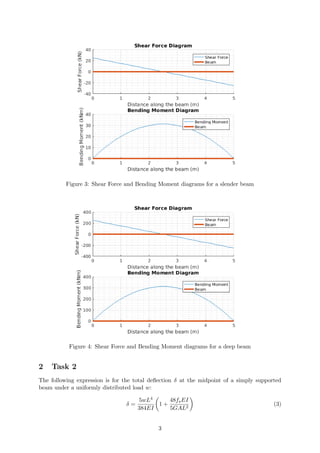
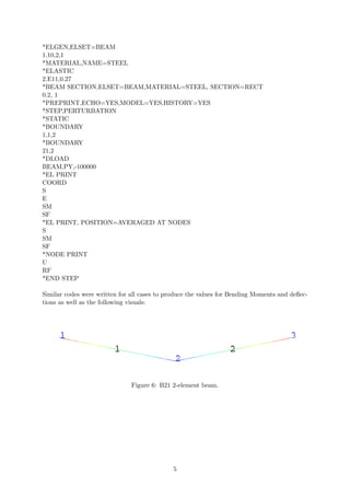
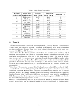
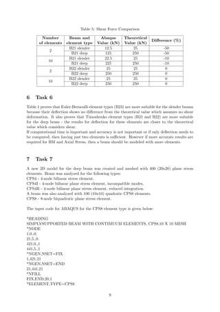
This document summarizes the analysis and modeling of slender and deep beams using finite element methods in ABAQUS. It compares the results from Euler-Bernoulli beam elements (B23) and Timoshenko beam elements (B21, B22) to theoretical solutions. For slender beams, the B23 element provides the most accurate deflection results compared to solutions that neglect shear deformation. For deep beams, the B22 element produces deflection results that most closely match solutions considering shear effects. In general, models with more elements provide more accurate bending moment and stress results.

1. University of Edinburgh
Finite Element Methods for Solids and Structures
Modelling of Shallow and Deep Beams
School of Engineering
Author:
Nadezda Avanessova s1449529
November 13, 2017

2. Contents
1 Task 1 2
2 Task 2 3
3 Task 3 4
4 Task 4 6
5 Task 5 8
6 Task 6 9
7 Task 7 9
8 Task 8 12
9 Task 9 17
10 Task 10 22
11 Task 11 24
12 Task 12 24
1

3. 1 Task 1
The plots of the shear force and bending moment were made in MATLAB using elementary
beam theory. Given beam is a simply supported beam, with a distributed load applied on top
of it 1. Starting from the left support and cutting the beam at a distance x from the support
Figure 1: Free Body Diagram of the Beam
(2) and applying the force equilibrium results in the following expressions for V (Shear Force)
and M (Bending Moment):
V = −wx + R (1)
M = −w
x2
2
+ Rx (2)
Figure 2: Cut Along the Beam
Where
R is the reaction force at the support - 25kN for a slender beam and 250kN for a deep beam,
w is the distributed load on the beam - 10kN for a slender beam and 100kN for a deep beam.
Plots in figures 3 and 4 were made for the slender and deep beam cases respectively.
2

4. Figure 3: Shear Force and Bending Moment diagrams for a slender beam
Figure 4: Shear Force and Bending Moment diagrams for a deep beam
2 Task 2
The following expression is for the total deflection δ at the midpoint of a simply supported
beam under a uniformly distributed load w:
δ =
5wL4
384EI
1 +
48fsEI
5GAL2
(3)
3

5. Where,
w is the distributed load on a beam which is equal to 10kN/m for a slender and 100kN/m for
a deep beam.
L is the length of a beam (m)
E is the Young’s modulus, which was taken as 200GPa, it is a typical value for structural
steel [1],
I is the moment of inertia which was calculated to be 133.33·106mm4 for a slender beam and
166.67·106mm4 for a deep beam.
A is the cross-sectional area of a beam,
fs = 6
5 is a form factor which for a rectangular section is equal to 6
5.
G is a shear modulus. For isotropic materials G can be found from the following formula:
G =
E
2(1 + υ)
(4)
Where
υ is a Poisson’s ratio which is equal to 0.27 for structural steel [1]. Equation 3 is considering shear
deformations. Expression in front of the brackets of this equation is representing the deflection
due to bending only. However if the beam is relatively thick an additional deflection will be pro-
duced by the shearing force, in the form of a mutual sliding of adjacent cross sections along each
other.
Figure 5: Shear Effect [2].
As a result of the non-uniform distribution of the shearing
stresses, the cross sections, previously plane, become curved as
in 5 which shows the bending due to shear alone. The elements
of the cross sections at the centroids remain vertical and slide
along one another [2]. Euler-Bernoulli beam theory assumes the
bending line is perpendicular to the cross-section of the beam
and hence the deflection equation would be:
δ =
5wL4
384EI
(5)
Timoshenko beam theory however allows a rotation between the
cross section and the bending line and hence considers the shear deformations, so that the
equation for deflection for the Timoshenko theory should be as presented in equation 3.
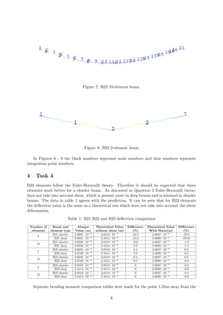
3 Task 3
The following describes the analysis of the slender and deep beams using Euler-Bernoulli (B23:
2-node cubic beam in a plane) and two types of Timoshenko elements (B21: 2-node linear beam
in a plane and B22: 3-node quadratic beam in a plane). The following represents an example
of the input for ABAQUS. This example was used to analyze the deep beam using Timoshenko
theory (B22) with 10 3-node quadratic elements.
*HEADING
SIMPLY SUPPORTED BEAM WITH CONTINUUM ELEMENTS, B22,10 ELEMENTS
*NODE
1,0.,0.
21,5.,0.
*NGEN
1,21,1
*ELEMENT,TYPE=B22
1,1,2,3
4

6. *ELGEN,ELSET=BEAM
1,10,2,1
*MATERIAL,NAME=STEEL
*ELASTIC
2.E11,0.27
*BEAM SECTION,ELSET=BEAM,MATERIAL=STEEL, SECTION=RECT
0.2, 1
*PREPRINT,ECHO=YES,MODEL=YES,HISTORY=YES
*STEP,PERTURBATION
*STATIC
*BOUNDARY
1,1,2
*BOUNDARY
21,2
*DLOAD
BEAM,PY,-100000
*EL PRINT
COORD
S
E
SM
SF
*EL PRINT, POSITION=AVERAGED AT NODES
S
SM
SF
*NODE PRINT
U
RF
*END STEP
Similar codes were written for all cases to produce the values for Bending Moments and deflec-
tions as well as the following visuals:
Figure 6: B21 2-element beam.
5

7. Figure 7: B22 10-element beam.
Figure 8: B23 2-element beam
In Figures 6 - 8 the black numbers represent node numbers and blue numbers represent
integration point numbers.
4 Task 4
B23 elements follow the Euler-Bernoulli theory. Therefore it should be expected that these
elements work better for a slender beam. As discussed in Question 2 Euler-Bernoulli theory
does not take into account shear, which is present more in deep beams and is minimal in slender
beams. The data in table 1 agrees with the prediction. It can be seen that for B23 elements
the deflection value is the same as a theoretical one which does not take into account the shear
deformation.
Table 1: B21 B22 and B23 deflection comparison
Number of
elements
Beam and
element type
Abaqus
Value (m)
Theoretical Value
without shear (m)
Difference
(%)
Theoretical Value
With Shear(m)
Difference
(%)
2
B21 slender 2.2987 · 10−3
3.0518 · 10−3
-24.7 3.0637 · 10−3
-25.0
B21 deep 2.0631 · 10−4
2.4414 · 10−4
-15.5 2.6800 · 10−4
-23.01
10
B21 slender 3.0328 · 10−3
3.0518 · 10−3
-0.6 3.0637 · 10−3
-1.0
B21 deep 2.6504 · 10−4
2.4414 · 10−4
8.5 2.6800 · 10−4
-1.1
2
B22 slender 3.0634 · 10−3
3.0518 · 10−3
0.4 3.0637 · 10−3
0.0
B22 deep 2.6749 · 10−4
2.4414 · 10−4
9.5 2.6800 · 10−4
-0.2
10
B22 slender 3.0634 · 10−3
3.0518 · 10−3
0.4 3.0637 · 10−3
0.0
B22 deep 2.6749 · 10−4
2.4414 · 10−4
9.5 2.6800 · 10−4
-0.2
2
B23 slender 3.0518 · 10−3
3.0518 · 10−3
0 3.0637 · 10−3
-0.4
B23 deep 2.4414 · 10−4
2.4414 · 10−4
0 2.6800 · 10−4
-8.9
10
B23 slender 3.0518 · 10−3
3.0518 · 10−3
0 3.0637 · 10−3
-0.4
B23 deep 2.4414 · 10−3
2.4414 · 10−3
0 2.6800 · 10−4
-8.9
Separate bending moment comparison tables were made for the point 1.25m away from the
6

8. pinned support and at the midpoint and values are presented in Tables 2 and 3 respectively.
Beams with 10 B23 elements show much better results than beams with only two elements. This
was expected - beams with more integration points give more accurate results. Considering all
these facts, for slender beams B23 element should be chosen.
Table 2: Bending Moment Comparison at 1.25m from the left end.
Number of
elements
Beam and
element type
Abaqus
Value (kNm)
Theoretical
Value (kNm)
Difference (%)
2
B21 slender 15.625 23.438 -33.3
B21 deep 156.250 234.375 -33.3
10
B21 slender 23.125 23.438 -1.3
B21 deep 231.250 234.375 -1.3
2
B22 slender 20.833 23.438 -11.1
B22 deep 208.330 234.375 -11.1
10
B22 slender 23.334 23.438 -0.4
B22 deep 233.335 234.375 -0.4
2
B23 slender 20.833 23.438 -11.1
B23 deep 208.330 234.375 -11.1
10
B23 slender 23.333 23.438 -0.4
B23 deep 233.333 234.375 -0.4
Table 3: Bending Moment Comparison in the middle of the beam.
Number
of elements
Beam and
element type
Abaqus
Value (kNm)
Theoretical
Value (kNm)
Difference (%)
2
B21 slender 15.625 31.25 -50
B21 deep 156.250 312.5 -50
10
B21 slender 30.625 31.25 -0.02
B21 deep 306.250 312.5 -0.02
2
B22 slender 36.458 31.25 16.7
B22 deep 364.580 312.5 16.7
10
B22 slender 31.460 31.25 0.7
B22 deep 314.600 312.5 0.7
2
B23 slender 36.460 31.25 16.7
B23 deep 364.600 312.5 16.7
10
B23 slender 31.458 31.25 0.7
B23 deep 314.580 312.5 0.7
ABAQUS can also provide the maximum and minimum axial stresses along the beam.
Maximum stresses at the midspan are compared to the theoretical value in Table 4. Axial
stress however depends on the bending moment (see Equation 6), therefore the values in the
’Difference (%)’ column are the same as for the Bending Moment.
7

9. Table 4: Axial Stress Comparison
Number
of elements
Beam and
element type
Abaqus
Value (MPa)
Theoretical
Value (MPa)
Difference (%)
2
B21 slender 11.72 23.44 -50
B21 deep 4.69 9.38 -50
10
B21 slender 22.97 23.44 -0.02
B21 deep 9.19 9.38 -0.02
2
B22 slender 27.34 23.44 16.6
B22 deep 10.94 9.38 16.6
10
B22 slender 23.59 23.44 0.6
B22 deep 9.44 9.38 0.6
2
B23 slender 27.34 23.44 16.6
B23 deep 10.94 9.38 16.6
10
B23 slender 23.59 23.44 0.6
B23 deep 9.44 9.38 0.6
5 Task 5
Timoshenko elements are B21 and B22. Similarly to Task 4, Bending Moments, Deflections and
Axial Stresses were compared. Because Timoshenko theory assumes shear, ABAQUS can also
provide shear forces to the user. Shear forces at the left end (pinned support) of the beam were
compared for B21 and B22 elements.
Table 1 shows that B21 element performs very badly in case when the beam consists of only 2
elements. The difference from theory for 2-element B21 case is bigger when compared to the
theoretical value considering shear than to that not considering shear. This is due to the fact
that there are only 2 elements. A beam consisting of only 2 elements and 2 integration points
cannot really generate any shear. For a 10-element case the results are better and match the
prediction. A deflection of a deep beam consisting of 10 B21 elements differs from the theoret-
ical value which considers shear by 1.1%. In terms of deflection B22 elements show the best
performance.
Tables 2 and 3 show that the accuracy of the Bending Moment and Axial Stress values is highly
dependent on the amount of integration points. The more integration points there are the more
accurate is the result. However when compared to Euler-Bernoulli results it may be noticed
that even though a B23 element has more integration points the difference from the theoretical
Bending Moment Value (and hence Axial Stress value as well) is the same for both B22 and
B23. This means that the average value between two integration points in B22 is very close to
the 3rd middle integration point value in B23.
Overall B22 performs better than B21 in all comparisons (Deflection, Bending Moment, Shear
Force). Table 5 shows that B22 elements provide the most accurate results for the shear force.
8

10. Table 5: Shear Force Comparison
Number
of elements
Beam and
element type
Abaqus
Value (kN)
Theoretical
Value (kN)
Difference (%)
2
B21 slender 12.5 25 -50
B21 deep 125 250 -50
10
B21 slender 22.5 25 -10
B21 deep 225 250 -10
2
B22 slender 25 25 0
B22 deep 250 250 0
10
B22 slender 25 25 0
B22 deep 250 250 0
6 Task 6
Table 1 proves that Euler-Bernoulli element types (B23) are more suitable for the slender beams
because their deflection shows no difference from the theoretical value which assumes no shear
deformation. It also proves that Timoshenko element types (B21 and B22) are more suitable
for the deep beam - the results for deflection for these elements are closer to the theoretical
value which considers shear.
If computational time is important and accuracy is not important or if only deflection needs to
be computed, then having just two elements is sufficient. However if more accurate results are
required for BM and Axial Stress, then a beam should be modeled with more elements.
7 Task 7
A new 2D model for the deep beam was created and meshed with 400 (20x20) plane stress
elements. Beam was analyzed for the following types:
CPS4 - 4-node bilinear stress element,
CPS4I - 4-node bilinear plane stress element, incompatible modes,
CPS4R - 4-node bilinear plane stress element, reduced integration.
A beam was also analyzed with 100 (10x10) quadratic CPS8 elements.
CPS8 - 8-node biquadratic plane stress element.
The input code for ABAQUS for the CPS8 element type is given below:
*HEADING
SIMPLYSUPPORTED BEAM WITH CONTIMUUM ELEMENTS, CPS8,10 X 10 MESH
*NODE
1,0.,0.
21,5.,0.
421,0.,1
441,5.,1
*NGEN,NSET=FIX
1,421,21
*NGEN,NSET=END
21,441,21
*NFILL
FIX,END,20,1
*ELEMENT,TYPE=CPS8
9

11. 1,1,3,45,43,2,24,44,22
*ELGEN,ELSET=EALL
1,10,2,1,10,42,10
*ELSET,ELSET=TOP,GENERATE
91,100,1
*MATERIAL,NAME=STEEL
*ELASTIC
2.E11,0.27
*SOLID SECTION,MATERIAL=STEEL,ELSET=EALL
.2
*PREPRINT,ECHO=YES,MODEL=YES,HISTORY=YES
*STEP,PERTURBATION
*STATIC
*BOUNDARY
1,1,2
*BOUNDARY
21,2
*DLOAD
TOP,P3,500000
*EL PRINT
COORD
S
E
*EL PRINT,POSITION=AVERAGED AT NODES
S
*NODE PRINT
U
RF
*END STEP
Figure 9 shows the exaggerated shapes for all 4 cases. Colors represent the magnitude of deflec-
tion, which is not symmetrical because elements can move in y-direction as well as x-direction in
the beam. CPS4R elements can produce an ’hourglass’ deformation pattern. Derived code for
ABAQUS can remove the ’hourglass’ effects. The deformed shape for that case is also presented
in Figure 9 and is named ”CPS4R with hourglass control”.
10

12. (a) CPS4
(b) CPS4I
(c) CPS4R
(d) CPS4R with hourglass control
(e) CPS8
Figure 9: Exaggerated Deformed Shapes for All Element Types.
As can be seen in Figure 9c a beam produced using CPS4R elements has ’hourglass’ at the
bottom of the beam. The reason for this is that CPS4R have a reduced number of integration
points.
11

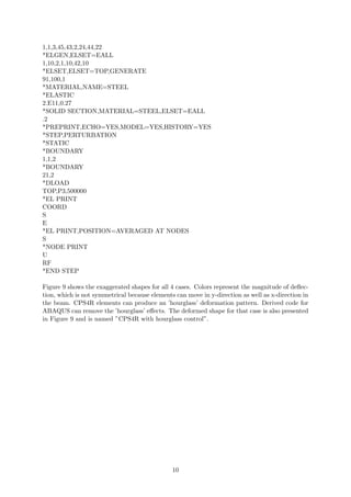
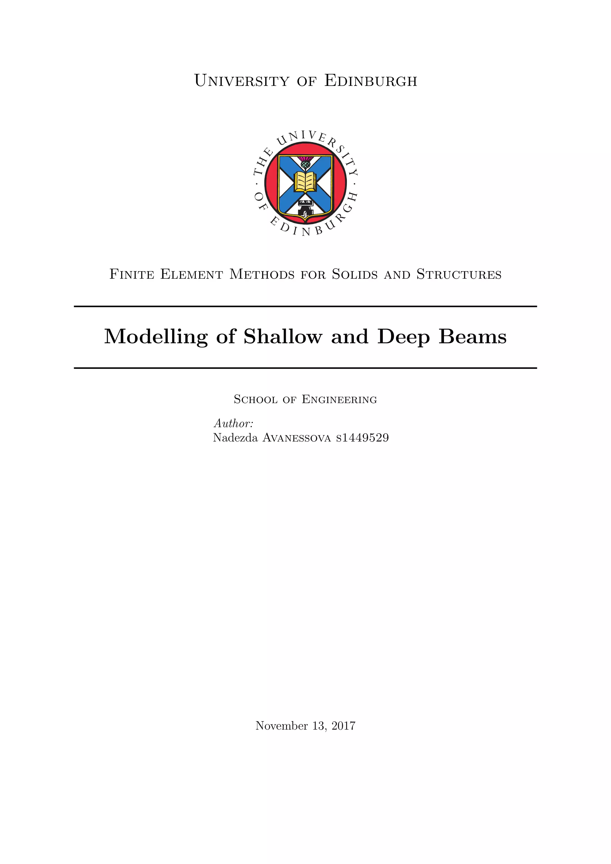
13. Consider a single reduced-integration element modeling a small piece of material subjected to
pure bending as shown in Figure 10. Neither of the dotted visualization lines has changed in
Figure 10: Bending of the single CPS4R element. [3]
length, and the angle between them is also unchanged, which means that all components of
stress at the element’s single integration point are zero. This bending mode of deformation is
thus a zero-energy mode because no strain energy is generated by this element distortion. The
element is unable to resist this type of deformation since it has no stiffness in this mode. In
coarse meshes this zero-energy mode can propagate through the mesh, producing meaningless
results. [3]
This element type can be used when the accuracy of the result is not so important to reduce
the computational time and to address the shear-locking effect [4].
8 Task 8
The bending stress can be derived from equation:
σ =
My
Ixx
(6)
Where
M is the bending moment at the point of interest which is 200kNm in this case,
y is is the distance from the neutral axis,
Ixx is the moment of inertia, which has been already calculated for this assignment.
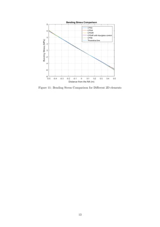
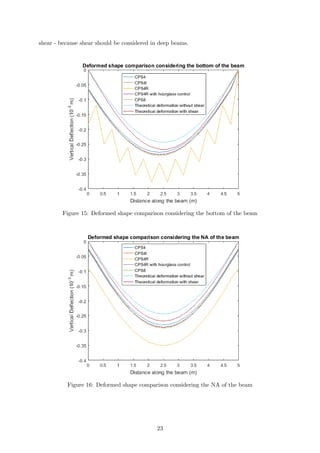
Theoretical line for the bending stress distribution was plotted in Figure 11 for the section
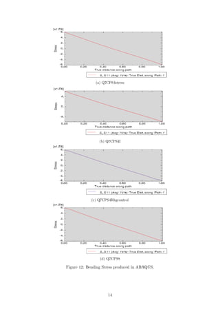
located 1m away from the pinned support. Stress plots were also observed using ABAQUS and
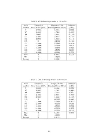
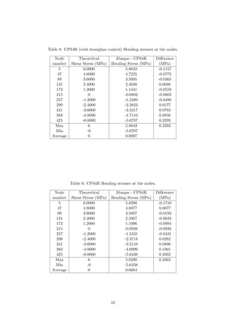
are shown in Figure 12. All stress distributions were plotted together in Figure 11. All values
both taken from ABAQUS .dat file and calculated for the theoretical line and their comparison
are provided in Tables 6 to 10. It can be seen that lines for all types of elements agree well with
the theoretical results. Stress distribution for CPS8 and CPS4I beam element types is match-
ing particularly well with the theory with maximum difference less than 0.2MPa (see Tables 6
to 10). It was predictable because these elements can better replicate the bending moments.
CPS4I element has a feature called incompatible modes. It is designed to avoid shear-locking
effect. The incompatible modes use more precise interpolation functions which model bending
better. It is the compromise in cost between the first- and second-order reduced integration
elements, with many of advantages of both [5].
In CPS4R case the distortion at the bottom of the beam (where y=-0.5) is most likely caused
by the ’hourglass’ effect. In case of CPS4R with hourglass control this distortion is absent.
Some errors might be caused by the fact that values from ABAQUS were taken at the nodes
(averaged at the nodes) and for better accuracy should be taken at the integration points.
12

14. Figure 11: Bending Stress Comparison for Different 2D elements
13

15. (a) Q7CPS4stress
(b) Q7CPS4I
(c) Q7CPS4Rhgcontrol
(d) Q7CPS8
Figure 12: Bending Stress produced in ABAQUS.
14

16. Table 6: CPS4 Bending stresses at the nodes.
Node
number
Theoretical
Shear Stress (MPa)
Abaqus - CPS4
Bending Stress (MPa)
Difference
(MPa)
5 6.0000 6.0055 0.0055
47 4.8000 4.7303 -0.0697
89 3.6000 3.4891 -0.1109
131 2.4000 2.2475 -0.1525
173 1.2000 1.0452 -0.1548
215 0 -0.1066 -0.1066
257 -1.2000 -1.2186 -0.0186
299 -2.4000 -2.3130 0.0870
341 -3.6000 -3.4180 0.1820
383 -4.8000 -4.5670 0.2330
425 -6.0000 -5.8248 0.1752
Max 6 6.0055 0.2330
Min -6 -5.8248
Average 0 0.0063
Table 7: CPS4I Bending stresses at the nodes.
Node
number
Theoretical
Shear Stress (MPa)
Abaqus - CPS4I
Bending Stress (MPa)
Difference
(MPa)
5 6.0000 6.1950 0.1950
47 4.8000 4.7997 -0.0003
89 3.6000 3.5833 -0.0167
131 2.4000 2.3331 -0.0669
173 1.2000 1.0955 -0.1045
215 0 -0.0962 -0.0962
257 -1.2000 -1.2442 -0.0442
299 -2.4000 -2.3704 0.0296
341 -3.6000 -3.5068 0.0932
383 -4.8000 -4.6925 0.1075
425 -6.0000 -5.9655 0.0345
Max 6 6.1950 0.1950
Min -6 -5.9655
Average 0 0.0119
15

17. Table 8: CPS4R (with hourglass control) Bending stresses at the nodes.
Node
number
Theoretical
Shear Stress (MPa)
Abaqus - CPS4R
Bending Stress (MPa)
Difference
(MPa)
5 6.0000 5.8843 -0.1157
47 4.8000 4.7225 -0.0775
89 3.6000 3.5695 -0.0305
131 2.4000 2.4038 0.0038
173 1.2000 1.1441 -0.0559
215 0 -0.0802 -0.0802
257 -1.2000 -1.2480 -0.0480
299 -2.4000 -2.3823 0.0177
341 -3.6000 -3.5217 0.0783
383 -4.8000 -4.7144 0.0856
425 -6.0000 -5.6707 0.3293
Max 6 5.8843 0.3293
Min -6 -5.6707
Average 0 0.0097
Table 9: CPS4R Bending stresses at the nodes.
Node
number
Theoretical
Shear Stress (MPa)
Abaqus - CPS4R
Bending Stress (MPa)
Difference
(MPa)
5 6.0000 5.8290 -0.1710
47 4.8000 4.8077 0.0077
89 3.6000 3.5807 -0.0193
131 2.4000 2.3367 -0.0633
173 1.2000 1.1006 -0.0994
215 0 -0.0926 -0.0926
257 -1.2000 -1.2431 -0.0431
299 -2.4000 -2.3718 0.0282
341 -3.6000 -3.5110 0.0890
383 -4.8000 -4.6999 0.1001
425 -6.0000 -5.6438 0.3562
Max 6 5.8290 0.3562
Min -6 -5.6438
Average 0 0.0084
16

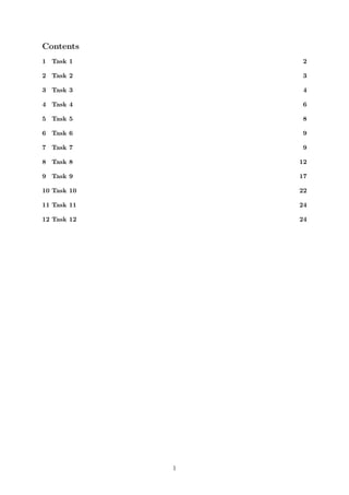
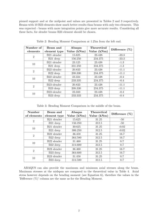
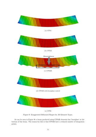
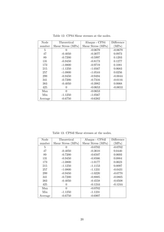
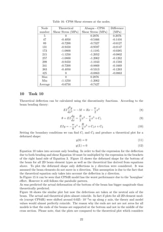
18. Table 10: CPS8 Bending stresses at the nodes.
Node
number
Theoretical
Shear Stress (MPa)
Abaqus - CPS8
Bending Stress (MPa)
Difference
(MPa)
5 6.0000 6.1753 0.1753
47 4.8000 4.6717 -0.1283
89 3.6000 3.5923 -0.0077
131 2.4000 2.4236 0.0236
173 1.2000 1.1958 -0.0042
215 0 -0.0275 -0.0275
257 -1.2000 -1.2228 -0.0228
299 -2.4000 -2.4001 -0.0001
341 -3.6000 -3.5899 0.0101
383 -4.8000 -4.8327 -0.0327
425 -6.0000 -6.1377 -0.1377
Max 6 6.1753 0.1753
Min -6 -6.1377
Average 0 -0.0138
9 Task 9
The theoretical plot for the shear stress can be obtained from the following equation:
τ =
6F · [(h/2)2 − y2]
b · h3
(7)
Where,
F is the shear force at the point of interest,
h is the hight of the beam,
b is the depth of the beam,
y is the distance from the NA.
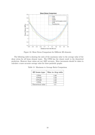
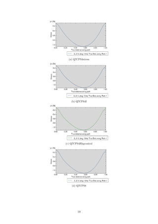
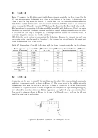
It is clear that the shape of the function should be parabolic and have maximum in the middle
of the beam i.e. NA (neutral axis). All shear stress distributions were plotted and analyzed
in the similar way to Task 8. Shear distributions are plotted together in Figure 13. It can be
seen clearly that the maximum value is not in the middle of the beam, however it is shifted
closer to the top of the beam. The reason for this is the fact that the beam is not supported in
the middle of the cross-section at every end, but the supports are located at the bottom of the
beam. In case if the supports are in the middle the shear stress distribution would agree with
the Beam Theory better. Also in Beam Theory one assumes that the loading occurs on the
neutral axis whereas in the model the distributed force is acting onto the top of the beam. The
discrepancy of the ABAQUS shear stress at the top and bottom of the beam (where y=0.5m
and y=-0.5m), occurs again due to the fact that the values were taken at the nodes and not at
the integration points.
17

19. Figure 13: Shear Stress Comparison for Different 2D elements
The following table is showing the ratio of the maximum value to the average value of the
shear stress for all beam element types. The CPS8 has the closest result to the theoretical
prediction. However these values are not 100% accurate. More increments should be taken to
calculate a more accurate average value for these parabolic graphs.
Table 11: Maximum to Average Ratio Comparison
2D beam type Max to Avg ratio
CPS4 1.66
CPS4I 1.63
CPS4R 1.62
CPS8 1.62
Theoretical value 1.5
18

20. (a) Q7CPS4stress
(b) Q7CPS4I
(c) Q7CPS4Rhgcontrol
(d) Q7CPS8
19

21. Table 12: CPS4 Shear stresses at the nodes.
Node
number
Theoretical
Shear Stress (MPa)
Abaqus - CPS4
Shear Stress (MPa)
Difference
(MPa)
5 0 -0.0679 -0.0679
47 -0.4050 -0.3077 0.0973
89 -0.7200 -0.5997 0.1203
131 -0.9450 -0.8173 0.1277
173 -1.0800 -0.9719 0.1081
215 -1.1250 -1.0567 0.0683
257 -1.0800 -1.0544 0.0256
299 -0.9450 -0.9494 -0.0044
341 -0.7200 -0.7316 -0.0116
383 -0.4050 -0.3982 0.0068
425 0 -0.0653 -0.0653
Max 0 -0.0653
Min -1.1250 -1.0567
Average -0.6750 -0.6382
Table 13: CPS4I Shear stresses at the nodes.
Node
number
Theoretical
Shear Stress (MPa)
Abaqus - CPS4I
Shear Stress (MPa)
Difference
(MPa)
5 0 -0.0702 -0.0702
47 -0.4050 -0.3610 0.0440
89 -0.7200 -0.6507 0.0693
131 -0.9450 -0.8566 0.0884
173 -1.0800 -1.0177 0.0623
215 -1.1250 -1.1153 0.0097
257 -1.0800 -1.1231 -0.0431
299 -0.9450 -1.0220 -0.0770
341 -0.7200 -0.8005 -0.0805
383 -0.4050 -0.4558 -0.0508
425 0 -0.1244 -0.1244
Max 0 -0.0702
Min -1.1250 -1.1231
Average -0.6750 -0.6907
20

22. Table 14: CPS4R Shear stresses at the nodes.
Node
number
Theoretical
Shear Stress (MPa)
Abaqus - CPS4R
Shear Stress (MPa)
Difference
(MPa)
5 0 0.0195 0.0195
47 -0.4050 -0.3161 0.0889
89 -0.7200 -0.7674 -0.0474
131 -0.9450 -0.8693 0.0757
173 -1.0800 -0.9891 0.0909
215 -1.1250 -1.0902 0.0348
257 -1.0800 -1.1145 -0.0345
299 -0.9450 -1.0273 -0.0823
341 -0.7200 -0.8113 -0.0913
383 -0.4050 -0.4624 -0.0574
425 0 -0.1240 -0.1240
Max 0 0.0195
Min -1.1250 -1.1145
Average -0.6750 -0.6866
Table 15: CPS4R (with hourglass control) Shear stresses at the nodes.
Node
number
Theoretical
Shear Stress (MPa)
Abaqus - CPS4R
Shear Stress (MPa)
Difference
(MPa)
5 0 -0.0682 -0.0682
47 -0.4050 -0.3610 0.0440
89 -0.7200 -0.6524 0.0676
131 -0.9450 -0.8565 0.0885
173 -1.0800 -1.0166 0.0634
215 -1.1250 -1.1144 0.0106
257 -1.0800 -1.1230 -0.0430
299 -0.9450 -1.0225 -0.0775
341 -0.7200 -0.8012 -0.0812
383 -0.4050 -0.4562 -0.0512
425 0 -0.1244 -0.1244
Max 0 -0.0682
Min -1.1250 -1.1230
Average -0.6750 -0.6906
21

23. Table 16: CPS8 Shear stresses at the nodes.
Node
number
Theoretical
Shear Stress (MPa)
Abaqus - CPS8
Shear Stress (MPa)
Difference
(MPa)
5 0 0.2076 0.2076
47 -0.4050 -0.5466 -0.1416
89 -0.7200 -0.7327 -0.0127
131 -0.9450 -0.9597 -0.0147
173 -1.0800 -1.1185 -0.0385
215 -1.1250 -1.2052 -0.0802
257 -1.0800 -1.2062 -0.1262
299 -0.9450 -1.1043 -0.1593
341 -0.7200 -0.8869 -0.1669
383 -0.4050 -0.5313 -0.1263
425 0 -0.0863 -0.0863
Max 0 0.2076
Min -1.1250 -1.2062
Average -0.6750 -0.7427
10 Task 10
Theoretical deflection can be calculated using the discontinuity functions. According to the
beam bending theory:
EI
d2y
dx2
= −M = Rx −
w
2
x2
(8)
θ = EI
dy
dx
=
R
2
x2
−
w
6
x3
+ C1 (9)
EIy = −
w
6
x4
+
R
6
x3
+ C1x + C2 (10)
Setting the boundary conditions we can find C1 and C2 and produce a theoretical plot for a
deformed shape:
y(0) = 0 (11)
y(L) = 0 (12)
Equation 10 takes into account only bending. In order to find the expression for the deflection
due to both bending and shear Equation 10 must be multiplied by the expression in the brackets
of the right hand side of Equation 3. Figure 15 shows the deformed shape for the bottom of
the beam for all 2D beam element types as well as the theoretical line derived from equations
above. To plot the deformed shape only deflections in y direction were considered. It was
assumed the beam elements do not move in x direction. This assumption is due to the fact that
the theoretical equation only takes into account the deflection in y direction.
In Figure 15 it can be seen that CPS4R model has the worst performance due to the ’hourglass’
effect. However it still follows the parabolic pattern.
As was predicted the actual deformation of the bottom of the beam has bigger magnitude than
theoretically predicted.
Figure 16 shows the similar plot but now the defections are taken at the neutral axis of the
beam. The actual and theoretical plots almost coincide. In fact if plots for all 2D element mod-
els (except CPS4R) were shifted around 0.025 · 10−3m up along y axis, the theory and model
values would almost perfectly coincide. The reason why the ends are not are not zeros for all
models is that the ends of the beams are supported at the bottom and not in the middle of the
cross section. Please note, that the plots are compared to the theoretical plot which considers
22

24. shear - because shear should be considered in deep beams.
Figure 15: Deformed shape comparison considering the bottom of the beam
Figure 16: Deformed shape comparison considering the NA of the beam
23

25. 11 Task 11
Table 17 compares the 2D deflections with the beam element results for the deep beam. For the
2D case, the maximum deflections were taken at the bottom of the beam. If deflections were
taken at the NA they would be smaller. It can be seen that the deflection of beam elements
B22 (both 2 and 10 element ones) have the closest maximum deflection value to the theoretical
value. Among the 2D model cases the CPS4 shows the closest to the theoretical value result.
The best choice for computing deflection would be beam B22 with 2 elements. If only the value
for deflection is needed, this beam element is sufficient enough and provides the accurate value.
It also does not take long to compute. 2D or multiple element beams are harder to model. It
also takes longer to compute the results for these.
CPS4R is the worst option for computing the deflection. Because its element has only one
integration point - as discussed in Question 7, the element has no stiffness in this mode and
hence deflects more than other models.
Table 17: Comparison of the 2D deflections with the beam element results for the deep beam.
Beam type and
number of elements
Abaqus Value
(10ˆ-3 m)
Theoretical Value
(10ˆ-3 m)
Difference
(%)
Theoretical value
Considering Shear
Difference
(%)
B21-2 2.0630
2.4414
-15.5
2.6800
-23.0
B21-10 2.6503 8.5 -1.1
B22-2 2.6748 9.5 -0.2
B22-10 2.6749 9.5 -0.2
B23-2 2.4414 0 -8.9
B23-10 2.4414 0 -8.9
CPS4 2.8109 15.1 4.9
CPS4I 2.8836 18.1 7.6
CPS4R 3.7771 54.7 40.9
CPS4R with
hour glass control
2.8890 18.3 7.8
CPS8 2.9219 19.7 9
12 Task 12
Symmetry can be used to simplify the problem and to reduce the computational complexity
and time. Appropriate model is shown in Figure 17. The beam is cut in the middle, the right
support stays as it was, the middle is restricted to move in x-direction to the left.In the model
considered in all previous cases all nodes except the first one (which is right at the pin support)
were allowed to move in x-direction. Roller support on the right will keep this condition true.
Degrees of freedom are shown in Figure 18. In case of a 2D model, every node on the left side
should be restricted in x-direction.
Figure 17: Reaction Forces on the redesigned model
24

26. Figure 18: Degrees of Freedom in the redesigned model
Figure 19: Redesigned model - 2D elements
25

27. References
[1] MatWeb, Material Property Data.
http://www.matweb.com/errorUser.aspx?msgid=2&ckck=nocheck
[2] S.Timoshenko, Strength of Materials. Part 1: Elementary Theory and Problems.
[3] Simulia, Getting Started With Abaqus: Interactive Addition..
[4] Eric Qiuli Sun, Shear Locking and Hourglassing in MSC Nastran, ABAQUS and ANSYS.
[5] ABAQUS, Presentation 10: Element Selection Criteria.
26