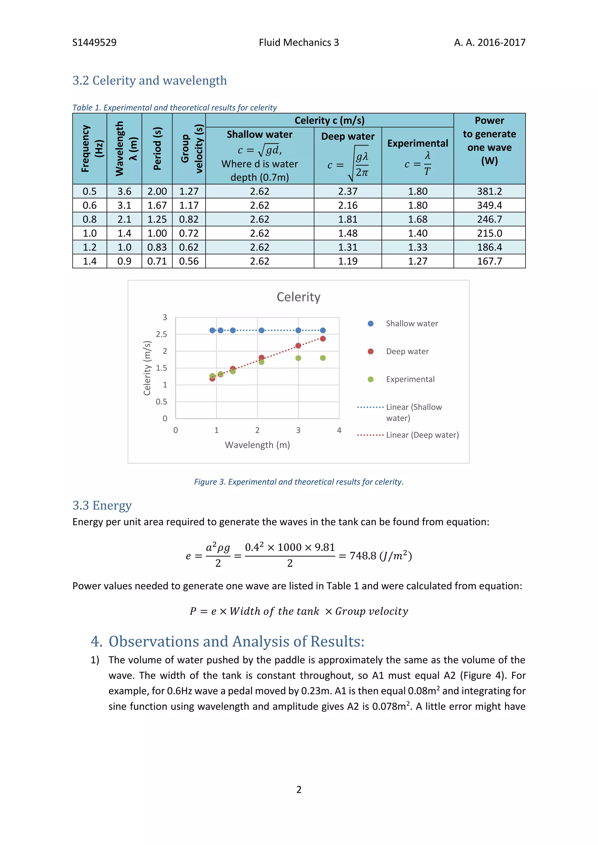
1) The document summarizes a lab report on wave tank experiments measuring wave properties like amplitude, period, and velocity under different conditions. Measurements were taken for waves between 0.5-1.4Hz. 2) Results showed that experimentally measured wave velocity followed deep water wave theory for wavelengths up to 3m, but followed shallow water wave theory for wavelengths over 3m. 3) Key observations included verifying theoretical predictions for wave and particle motion, as well as demonstrating breaking waves formed by interference of different frequency waves.

1. WAVE TANK LAB REPORT
Fluid Mechanics 3
University of Edinburgh
Nadezda Avanessova
S1449529
17/04/2017

2. S1449529 Fluid Mechanics 3 A. A. 2016-2017
1
1. Introduction
The aim of this experiment is to compare waves of different frequency observed in the lab with
theoretical prediction for shallow and dep water waves. Some observations from the laboratory
experiment are also mentioned and analysed in this report.
2. Methodology
The experiment is set up so that there is a 0.4m wide tank filled with water. Water is pushed by an
oscillating pedal at one end of the tank controlled by software to simulate waves (Figure 1– right). The
opposite end of the tank has a sponge and a net to absorb the energy of the wave. Software allows to
vary frequency from 0.5Hz to 1.4Hz or combine them to crate breaking waves. For lower frequency
the pedal oscillates slower but with higher amplitude. Several measurements were made in this
experiment:
 Wave amplitude
 Pedal amplitude
 Group velocity
 Travelling speed in terms
of waves per second
 Dimensions of the tank
Even though the wavelength can
be calculated using Group velocity
and a travelling speed (waves per
second) and the length of the tank
(14m) it was decided that more accurate values can be obtained with the photos of every wave.
Between experiments a pedal was switched off to allow water to settle down so that there would be
no disturbance between the waves.
To observe the circulation a few pieces of tissue were dropped into the tank.
3. Results:
3.1 Wave period
𝑊𝑎𝑣𝑒 𝑝𝑒𝑟𝑖𝑜𝑑 𝑇 =
1
𝑓
, 𝑤ℎ𝑒𝑟𝑒 𝑓 𝑖𝑠 𝑤𝑎𝑣𝑒 𝑓𝑟𝑒𝑞𝑢𝑒𝑛𝑐𝑦
Output tables of the software
provided in the Lab show the
variation of voltage for every
of four gauges in the water
tank (Figure 1 – left). Because
they are not calibrated
properly the results for all
gauges do not match. An
example for 0.6Hz is shown in
Figure 2:
.
Figure 1. Wave tank.
Figure 2. Output from gauges.

3. S1449529 Fluid Mechanics 3 A. A. 2016-2017
2
3.2 Celerity and wavelength
Table 1. Experimental and theoretical results for celerity
Frequency
(Hz)
Wavelength
λ(m)
Period(s)
Group
velocity(s)
Celerity c (m/s) Power
to generate
one wave
(W)
Shallow water
𝑐 = √𝑔𝑑,
Where d is water
depth (0.7m)
Deep water
𝑐 = √
𝑔𝜆
2𝜋
Experimental
𝑐 =
𝜆
𝑇
0.5 3.6 2.00 1.27 2.62 2.37 1.80 381.2
0.6 3.1 1.67 1.17 2.62 2.16 1.80 349.4
0.8 2.1 1.25 0.82 2.62 1.81 1.68 246.7
1.0 1.4 1.00 0.72 2.62 1.48 1.40 215.0
1.2 1.0 0.83 0.62 2.62 1.31 1.33 186.4
1.4 0.9 0.71 0.56 2.62 1.19 1.27 167.7
Figure 3. Experimental and theoretical results for celerity.
3.3 Energy
Energy per unit area required to generate the waves in the tank can be found from equation:
𝑒 =
𝑎2
𝜌𝑔
2
=
0.42
× 1000 × 9.81
2
= 748.8 (𝐽/𝑚2
)
Power values needed to generate one wave are listed in Table 1 and were calculated from equation:
𝑃 = 𝑒 × 𝑊𝑖𝑑𝑡ℎ 𝑜𝑓 𝑡ℎ𝑒 𝑡𝑎𝑛𝑘 × 𝐺𝑟𝑜𝑢𝑝 𝑣𝑒𝑙𝑜𝑐𝑖𝑡𝑦
4. Observations and Analysis of Results:
1) The volume of water pushed by the paddle is approximately the same as the volume of the
wave. The width of the tank is constant throughout, so A1 must equal A2 (Figure 4). For
example, for 0.6Hz wave a pedal moved by 0.23m. A1 is then equal 0.08m2
and integrating for
sine function using wavelength and amplitude gives A2 is 0.078m2
. A little error might have
0
0.5
1
1.5
2
2.5
3
0 1 2 3 4
Celerity(m/s)
Wavelength (m)
Celerity
Shallow water
Deep water
Experimental
Linear (Shallow
water)
Linear (Deep water)

4. S1449529 Fluid Mechanics 3 A. A. 2016-2017
3
been caused by inappropriate set up of a pedal – it moved
to one side more than another because the water level
was lower than required.
2) Due to a very small discrepancies with theory it was
concluded that wave absorber in this experiment was
efficient. The absorbent however oscillated more at longer
wavelengths. The effectiveness of energy absorption could
be increased with longer span and damping improvement
of the absorber, so that it would not oscillate and cause
disturbance.
3) Tissue particles behaved in water as was expected by Stokes drift. Particles’ motion path was
circular. The rotation velocity decreased with depth and hence the circular path shrinks until
the tissue reaches the ground – but even then it continues to move backwards and forwards.
4) Experiment has shown the Stokes drift in action. It was observed that once a wave is created,
it does not change it shape but rather travels linearly along the tank together with the group
of waves until it gets absorbed. An exception was a break wave.
5) In the real sea or ocean waves usually have different frequencies what causes breaking waves.
The generation of breaking wave is
programmed in the software. Here
is the process of creating such
wave: the pedal starts generating a
high frequency wave which moves
slowly down the tank and is
followed by a low frequency wave
which travels faster, once they
catch up they superimpose and at
some point the wave becomes so
high that it brakes (Figure 5).
6) Capillary waves were observed at
water surface. These are the
waves of wavelengths smaller
than 1cm and which are majorly
affected by water surface tension
(Figure 6).
7) Experimentally obtained celerity
seems to follow the theoretical
line for deep water waves up to
the wavelength of around 3m or frequency of 0.6Hz. After this value it does not show any
change with increase of wavelength which is characteristic to shallow water theory. To sum
up, 0.8-1.4Hz waves obey deep water theory while 0.5-0.6Hz waves are closer to shallow
water theory or can be assumed to be in transition region.
Figure 4
Figure 5. Breaking waves.
Figure 6. Capillary waves.