Fem based modelling of amb control system 2

International Journal of Mechanical Engineering and Technology (IJMET), ISSN 0976 –
6340(Print), ISSN 0976 – 6359(Online) Volume 4, Issue 3, May - June (2013) © IAEME
191
FEM BASED MODELLING OF AMB CONTROL SYSTEM
Madhura.S†
, Pradeep B Jyoti††
, Dr.T.V.Govindaraju†††
,
†
lecturer, Mechanical Engineering Department, ShirdiSai Engineering College, Bangalore,
India
††
Head of The Electrical Engineering Department, ShirdiSai Engineering College, Bangalore,
India
†††
Principal, ShirdiSai Engineering College, Bangalore, India
ABSTRACT
Active Magnetic Bearing (AMB) sustains a rotor by magnetic attractive forces,
exclusive of any mechanical contact. This paper illustrates a field-circuit design of an active
magnetic bearing in conjunction with its control loop. The primary and underlying
specifications of the active magnetic system have been realized from a FEM study of a
magnetic bearing actuator. The position control system is grounded on working dynamics of
the local accustomed PID controller, which has been extensively employed in manufactories
oriented employment of the active magnetic bearing systems. The specifications of the
controller have been acquired by exploiting the root locus method. The realized simulation
and experimental outcomes are evaluated in event of lifting the rotor.
Keywords: Modelling, control system, magnetic bearing control system, Finite Element
Method, controller, simulation, rotor, levitation control algorithm, force, flux density transfer
function, transmittance.
1. INTRODUCTION
Active magnetic bearings assert employment in abstruse and industrial appliances to
sustain the contactless levitation of the rotor. Resolute working of apparatuses and machines,
which comprise of active magnetic bearings are realized by virtue of appurtenant magnetic
forces developed by the magnetic bearing actuator. Magnetic bearings have quite a few
leverages over mechanical and hydrostatic ones. The uttermost important improvements are
INTERNATIONAL JOURNAL OF MECHANICAL ENGINEERING
AND TECHNOLOGY (IJMET)
ISSN 0976 – 6340 (Print)
ISSN 0976 – 6359 (Online)
Volume 4, Issue 3, May - June (2013), pp. 191-202
© IAEME: www.iaeme.com/ijmet.asp
Journal Impact Factor (2013): 5.7731 (Calculated by GISI)
www.jifactor.com
IJMET
© I A E M E

192
[9]: contactless dynamics and exemption from lubrication and contamination wear. The rotor
may be conceded to rotate at high speed; the immense circumferential speed is only
restrained by the tenacity and stableness of the rotor material and constituents. At high
operation speeds, friction losses are diminished by 5 to 20 times than in the prevailing ball or
journal bearings. Considering the dearth of mechanical wear, magnetic bearings have
superior life span and curtailed maintenance expenditure. Nonetheless, active magnetic
bearings also have its shortcomings. The contrivance of a magnetic bearing system for a
specialized employment necessitates proficiency in mechatronics, notably in mechanical and
electrical engineering and in information processing. Owing to the intricacies of the magnetic
bearing system, the expenses of procurement are considerably larger vis-a-vis conventional
bearings. Howbeit, on account of its many superiorities, active magnetic bearings have
asserted acceptance in many industrial applications, such as turbo-molecular vacuum pumps,
flywheel energy storage systems, gas turbines, compressors and machine tools.
With the aid of this thesis, the dynamic behavior of an active magnetic bearing has
been scrutinized. The illustrated dynamic model is grounded on the coil inductance, the
velocity-induced voltage coefficient and the radial force characteristic, which are computed
by the finite element method.
2. MODELLING OF THE ACTIVE MAGNETIC BEARING
2.1 Specification
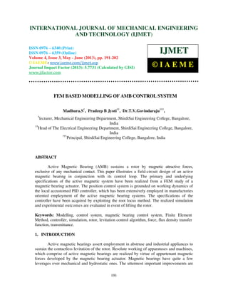
The deliberate levitation actuator produces a 12-pole heteropolar bearing. The
magnetic system has been fabricated from laminated sheets of M270-50 silicon steel.
Organization of the 12-pole system is disparate from the 8-pole archetypical bearings. The
attractive force produced in y-axis is twice the force generated in the x-axis. The four control
windings of the 12-pole bearing, exhibited in Figure 1, comprises of 12 coils connected
thusly: 1A-1B-1C-1D,2A-2B, 3A-3B-3C-3D and 4A-4B. The windings 1 and 3 generates the
attractiveforce along the y -axis, albeit windings 2 and 4 generate magnetic force in the x-
axis. The physical characteristics of the active magnetic bearing have been exhibited in Table
1.
TABLE 1
Specification of the radial active magneticbearing parameters
Property Value
Number of Poles 12
Stator axial length 56 mm
Stator outer diameter 104 mm
Stator inner diameter 29 mm
Rotor axial length 76 mm
Rotor diameter 28 mm
Nominal air gap 1 mm
Number of turns per pole 40
Copper wire gauge 1 mm2
Stator weight 2.6 kg
Current stiffness coefficient 13 N/A
Position Stiffness coefficient 42 N/mm

193
Fig. 1. Front view of the active Magnetic bearing
Fig. 2. B-H characteristic for the laminated ferromagnetic material M270-50
2.2. Modelling of the active magnetic bearing actuator
Active magnetic bearing is an archetypical electromagnetic system where the
electrical and mechanical energies are conjugated by the magnetic field. A dynamic
representation of the active magnetic bearing in y-axis is governed by the assortment of
ordinary differential equations:
(1)
(2)
dt
dy
h
dt
di
LiRu vd 1
1
1111 ++=
dt
dy
h
dt
di
LiRu d ++= 1
3333
),(2
2
yiF
dt
yd
m cyy=

International Journal of Mechanical Engineering and Technology (IJMET), ISSN 0976
6340(Print), ISSN 0976 – 6359(Online) Volume 4, Issue 3, May
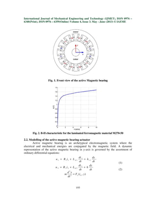
The voltage equations (1) actuates the electrical comportment of the active magnetic
bearing, wherein u1, u 3 are the sup
ones: i1 = iby + icy, i3 = iby - icy. R1, R3 are the winding’s resistances, Ld1, L d3 designate
the dynamic inductances of the windings and hv1, hv3 elucidates the velocity
voltage. The mechanical equations (2) actuates the dynamic model of the magnetically
suspended shaft.
An active magnetic bearing is identified by the nonlinear affiliation between the
attractive force and position of the rotor and windings currents.
Scrutinizing the opposing pair of the electromagnets the subsequent linear correlation for the
attractive force can be realized:
Fy= kiyicy
The current stiffness coefficient
as partial derivatives of the radial force
, )(
=
∂
∂
=
oycv
cvv
iv
i
yiF
k
The fundamental specifications of the active magnetic bearing actuator have been
enumerated using FEM analysis. Simulation of the magnetic bearing was actualized with
Matlab/Simulink software. The block diagram of the AMB model in the
circuit method is illustrated in Figure 3. The constituents of the block “Electromagnets 1 and
3” is shown in Figure 4.
Fig. 3. Block diagram
6359(Online) Volume 4, Issue 3, May - June (2013) © IAEME
194
bearing, wherein u1, u 3 are the supply voltages, the currents i1, i3 consist of bias and control
icy. R1, R3 are the winding’s resistances, Ld1, L d3 designate
the dynamic inductances of the windings and hv1, hv3 elucidates the velocity
mechanical equations (2) actuates the dynamic model of the magnetically
attractive force and position of the rotor and windings currents.
pposing pair of the electromagnets the subsequent linear correlation for the
cy ksy y
The current stiffness coefficient kiy and position stiffness coefficient ksy
of the radial force Fy, [10]:
0
, )(
,
=∂
∂
=
cvi
cvv
sv
y
yiF
k
link software. The block diagram of the AMB model in the y-axis for the field
Fig. 3. Block diagram for the analysis of the AMB dynamics in y-axis
June (2013) © IAEME
of bias and control
icy. R1, R3 are the winding’s resistances, Ld1, L d3 designate
the dynamic inductances of the windings and hv1, hv3 elucidates the velocity-induced
mechanical equations (2) actuates the dynamic model of the magnetically
pposing pair of the electromagnets the subsequent linear correlation for the
(3)
are construed
(4)
axis for the field-
axis

6340(Print), ISSN 0976 – 6359(Online) Volume 4, Issue 3, May
Fig. 4. The content
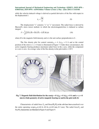
2.3. Finite element computation of AMB
Magneto static estimation of magnetic field distribution in the magnetic bearing was
executed by 2D Finite Element Method, employing the program FEMM 4.2 [8]. The problem
is formulated by Poisson’s equation:
Whereµ is the permeability of material,
potential in z direction, J is the current density. In the calcu
characteristics µ(B) of the ferromagnetic material, illustrated in
mock up of the active magnetic bearing has been discredited by 82356 standard triangular
6359(Online) Volume 4, Issue 3, May - June (2013) © IAEME
195
Fig. 4. The content of the block Electromagnets 1 and3"
2.3. Finite element computation of AMB
ecuted by 2D Finite Element Method, employing the program FEMM 4.2 [8]. The problem
is formulated by Poisson’s equation:
is the permeability of material, B is the magnetic flux density, A is the magnetic
is the current density. In the calculation incorporates nonlinear
) of the ferromagnetic material, illustrated in Figure 2. A two
JA
B
=








×∇×∇
µ
1
June (2013) © IAEME
ecuted by 2D Finite Element Method, employing the program FEMM 4.2 [8]. The problem
the magnetic vector
lation incorporates nonlinear
Figure 2. A two-dimensional

196
elements(Fig. 5a). Computation of the magnetic bearing forces by the Maxwell's stress tensor
method necessitates a closed surface that envelopes the rotor in free space [1]. For that
reason, the air gap area was split into two subareas amidst stator and rotor (Fig. 5b). In
consideration of solving equation (5) the boundary conditions have to be ascertained. As a
result, on the outer edges of the calculation area Dirichlet boundary conditions have been
assumed.
Fig. 5.Discretization of the model Fig. 6. The finite element mesh in the
subregions of stator and rotor
In light of equation (5) solution, the circulation of the Az component for magnetic vector
potential has been realized. Consequently, the vector of magnetic field distribution is
ascertained as:
(6)
Assuming the 2D field, the magnetic flux of the coils has been calculated from:
(7)
whereN connotes the number of turns of the coil, Az,i+ and Az,i- are the vector potentials on the
positive and negative sides of the coil turn, correspondingly.
The dynamic inductance is calculated as partial derivative of the flux with respect to
the current i:
ol
Ld
ψ∂
= (8)
y
z
x
z
x
A
y
A
B 11
∂
∂
−
∂
∂
=
)(.
1 1
1 −
= =
+ −==Ψ ∑∫ ∑ zj
N
i l
N
i
zj AAldlA

197
while the velocity-induced voltage is derived as partial derivative of the flux with respect to
the displacement s:
os
hv
ψ∂
= (9)
The displacement "s" connotes "y" or "x" movement. The radial force is derived by
Maxwell's stress tensor method, in which the electromagneticforce is deduced as surface
integral:
dsBHnHnBBnHF )}.().().({
2
1
−+= ∫ (10)
where H is the magnetic field intensity and n is the unit surface perpendicular to S .
The flux density plot for control currenticy = 4 A,icx = 0 A and at the central
position of the rotor (x = y = 0 mm) is illustrated in Figure 7. Under these circumstances, the
active magnetic bearing produces maximum radial force in the y-axis, while the component
in x-axis is zero. An average value of the flux density in the pole tooth is 1.30 T.
Fig. 7. Magnetic field distribution for the caseib = 4 A,icy = 4 A,icx = 0 A and x = y = 0
mm in whole geometry of active magnetic bearing (a) and in the pole teeth (b)
Characteristics of radial force Fy and fluxesΨ1,Ψ3 in the coils have been actualized over
the entire operating scopeicy∈(-4.0 A, 4.0 A), y∈(-0.3 mm, 0.3 mm). The radial forceFy and
fluxΨ1characteristicsareillustratedinFigure 8 and Figure 9.

198
Fig. 8. Radial force characteristicFy(icy,y) Fig. 9. Flux characteristicΨ1(icy,y)
Fig. 10. Dynamic inductance Fig. 11. The velocity-induced voltage
characteristicLd1(icy,y) characteristic hv1(icy,y)
2.4. Control system for the Active Magnetic Bearing
Lately there have been new developments and improvisation of various algorithms to
manipulate the active magnetic bearings. The most decisive and momentous ones are: PID
control [4], gain scheduled control [2], robust H∞ control [6], LQ control [11], fuzzy logic
control [5], feedback linearization control [7]. Regardless of comprehensive and accelerated
development of the advanced control algorithms for the active magnetic bearing, the
industrial applications of the magnetic bearing were generally grounded on digital or analog
PID controllers.
The transformation function of the current controlled active magnetic bearing in y-
axis is governed by the following equation:
sv
iv
AMB
kms
k
sG
−
= 2
)( (11)

199
The poles of the transfer function exemplifies an unstable system, since one of the
poles has a positive value. Therefore, the active magnetic bearing necessitates a control
system. Stable fuctioning can be realized with decentralized PID controller, with the transfer
function [3]:
DIpPID sKKKsG s
++=)( (12)
The block diagram of the control system with PID controller for y-axis is illustrated
in Figure 12, whereyr(t) connotes the reference value of the rotor position (generally equal to
zero),icy(t) is the reference control current and y(t) is position of the rotor.
Fig. 12. Block diagram of the control system
Laplace transfer function of the closed loop is described by the transmittance:
(13)
The closed-loop system with the PID controller has three polesλ1,λ2,λ3. To deduce the
magnitude of KP, KI, KD, the coefficients of the denominator of GCL(s) in Eq. 13 should be
evaluated against coefficients of the polynomial form:
321313221
2
321
3
)()( λλλλλλλλλλλλ +++++++ sss (14)
As a result, the specifications of the PID controller are equal to:
iv
p
k
K
)( 133221 λλλλλλ ++
= (15)
iv
I
k
m
K 321 λλλ
=
iyD kmK }){( 321 λλλ −−−=
Position of the polesλ1,λ2,λ3 in the s-plane influences the characteristicsof the transients. According to
the pole placement method [4] two poles can be determined from:
21 1 ζωζωλ −+−= nn i
22 1 ζωζωλ −+−= nn i (16)
m
kK
S
m
Kpk
S
m
kK
S
m
kK
S
m
Kpk
S
m
kK
sG
iyIiyiyD
iyIiyiyD
CL
+++
++
=
23
2
)(

200
Where inωnistheundamped naturalfrequency:
ζ
ω
s
n
t
6.4
= (17)
The third pole of transfer function of GCL(s) should be positioned outside the
dominant area. Subsiquently, the coefficients KP, KI, KD rely on the settling timetS and
damping ratioζ.
3. SIMULATION AND EXPERIMENTAL RESULTS
To stabilize the rotor two decoupled PID controllers were employed. The control
tasks have been accomplished with 32-bit microcontroller with very proficient ARM7TDMI-
S core. The sampling frequency of PID controllers are equal to 1 kHz. The location of the
rotor is measured by Turck contact-less inductive sensor with bandwidth 200 Hz. The analog to
digital converters resolution equals 2.44µm. The parameters of PID controllers were determined
according to the proposed method for the settling time tS = 50 ms and the damping
coefficientζ=0.5.The values of parameters of PID controllers are shown in Table 2.
TABLE 2
Parameters of the PID controller
KP[A/m] KI[A/ms] KD[ms/m]
11231 514080 45
Figures 13 and 14 illustrate the contrast of simulated and experimental outcomes
throughout rotor lifting. The curve characters of the properties are close to the measured ones.
It is evident that the current value in the steady state is marginally higher than in the real
system.
Fig. 13.Time response of currenti1 Fig. 14. Time response of the AMB shaft
displacement in y-axis

201
The transient state for the rotor position for both systems diversifies, owing to the fact
that the settling time in the simulated system is shorter than in the real one. Contrarieties are
result of the simplified modelling of the magnetic bearing's actuator, specifically because of
overlooking the hysteresis phenomena and the fringing effect.
4. REMARKS AND CONCLUSION
This thesis demonstrates a modus-operandi for designing control systems for active
magnetic bearings. The dynamic behavior of active magnetic bearings has been realized from a
field-circuit model. The fundamental parameters of the active magnetic bearing actuator have
been deduced using FEM analysis .
The illustrated technique for designing PID controllers makes manipulating the
controller specifications simpler and promises acceptable damping.
LITERATURE
[1.] Antila M., Lantto E., Arkkio A.: Determination of Forces and Linearized Parameters
of Radial Active Magnetic Bearings by Finite Element Technique, IEEE Transaction
On Magnetics, Vol. 34, No. 3, 1998, pp. 684-694.
[2.] Betschon F., Knospe C.R.: Reducing magnetic bearing currents via gain scheduled
adaptive control, IEEE/ASME Transactions on Mechatronics, Vol. 6, No. 4, 12.2001,
pp. 437-443.
[3.] FranklinG.: Feedback control of dynamic systems, Prentice Hall, New Jersey, 2002.
[4.] Gosiewski Z., Falkowski K.: Wielofunkcyjneło yskamagnetyczne,
BibliotekaNaukowa InstytutuLotnictwa, Warszawa, 2003.
[5.] Hung. J.Y.: Magnetic bearing control using fuzzy logic, IEEE Transactions on
Industry Applications, Vol. 31, No. 6, 11.1995, pp. 1492-1497.
[6.] Lantto E.: Robust Control of Magnetic Bearings in Subcritical Machines, PhD thesis,
Espoo, 1999.
[7.] Lindlau J., Knospe C.: Feedback Linearization of an Active Magnetic Bearing With
Voltage Control, IEEE Transactions on Control Systems Technology, Vol. 10, No.1,
01.2002, pp. 21-31.
[8.] Meeker D.: Finite Element Method Magnetics Version 4.2, User's Manual, University
of Virginia, U.S.A, 2009.
[9.] Schweitzer G., Maslen E.: Magnetic Bearings, Theory, Design and Application to
Rotating Machinery, Springer, Berlin, 2009.
[10.] Tomczuk B., Zimon J.: Filed Determination and Calculation of Stiffness Parameters in
an Active Magnetic Bearing (AMB), Solid State Phenomena, Vol. 147-149, 2009, pp.
125-130.
[11.] Zhuravlyov Y.N.: On LQ-control of magnetic bearing, IEEE Transactions On Control
Systems Technology, Vol. 8, No. 2, 03.2000, pp. 344-355.
[12.] H. Mellah and K. E. Hemsas, “Design and Simulation Analysis of Outer Stator Inner
Rotor Dfig by 2d and 3d Finite Element Methods”, International Journal of Electrical
Engineering & Technology (IJEET), Volume 3, Issue 2, 2012, pp. 457 - 470,
ISSN Print : 0976-6545, ISSN Online: 0976-6553.
[13.] Siwani Adhikari, “Theoretical and Experimental Study of Rotor Bearing Systems for
Fault Diagnosis”, International Journal of Mechanical Engineering & Technology
(IJMET), Volume 4, Issue 2, 2013, pp. 383 - 391, ISSN Print: 0976 – 6340, ISSN
Online: 0976 – 6359.

202
AUTHORS DETAIL
Madhura.S
Obtained her BE from Visveswaraya Technological University in the
year 2008, ME in Machine Design from Anna University. Coimbatore
in the year 2011.Currently Pursuing Ph.D – Failure analysis of Active
Magnetic Bearing and its correction using smart controller under the
guidance of Dr.T.V.Govindaraju.Field of interest Machine design,
FEM techniques and mechatronics.
Pradeep B Jyoti
Graduated from Karnataka University Dharwad, Karnataka in the year
1986, M.E from Gulbarga University, Gulbarga in the year 1989. He
is currently pursuing Ph.D at Jawaharlal Nehru Technological
University, Hyderabad, India. He is presently working as Professor &
Head in the Department of Electrical and Electronics ShirdiSai
Engineering College, Bangalore, Karnataka, India. His research areas
include SVPWM techniques, and Vector control of electrical drives &
machines.
Dr.T.V.Govindaraju
Obtained his Ph.D in the field of” experimental techniques (photo
elasticity)” in the year 2000 from Bangalore University. His current
field of interest are Machine design, FEM techniques and
Mechatronics. Presently involved in guiding Research scholars leading
to Ph.D program.

Fem based modelling of amb control system 2

More Related Content

What's hot

Viewers also liked

Similar to Fem based modelling of amb control system 2

More from IAEME Publication

Recently uploaded

Fem based modelling of amb control system 2