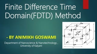
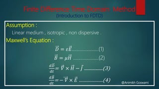
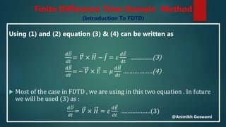
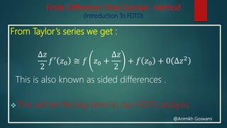
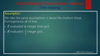
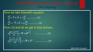
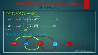
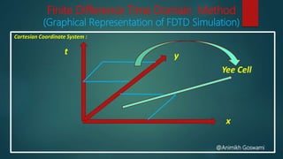
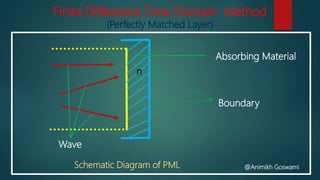
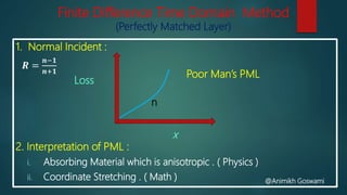
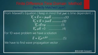
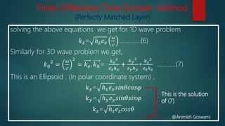
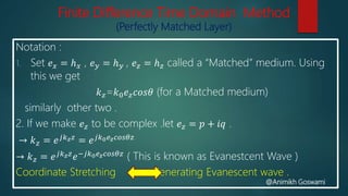
The document discusses the finite difference time domain (FDTD) method, a widely used computational electromagnetic technique foundationally developed by Yee in 1966. It covers essential topics such as the formulation in two dimensions, time stepping, and the concept of perfectly matched layers to absorb waves in simulations. Key equations from Maxwell's equations are utilized throughout, along with assumptions about the medium being linear and isotropic.

1. Finite Difference Time
Domain(FDTD) Method
- BY ANIMIKH GOSWAMI
Department of Nanoscience & Nanotechnology ,
University of Kalyani

2. Declaimer
Before going to Finite Difference Time Method (FDTD)
(FDTD) we should know about the following topic :
 Vector Algebra and Vector Calculus
 Different form of Maxwell’s equation and their
solving.
 Interpolation and Numerical Analysis
 Finite Difference Method
 Computer Programming
@Animikh Goswami

3. Finite Difference Time Domain Method
Contents :
 Introduction to FDTD
 2D Formulation
 Time Stepping
 Perfectly Matched Layer(PML)
@Animikh Goswami

4. Finite Difference Time Domain Method
(Introduction to FDTD)
History and Central Idea :
 Simplest and most widely used Computational Electromagnetic
method.
 Yee (1966) lead the foundation .
 Very useful for Time domain formulation : Wave Propagation ,
Pulsed transient phenomena . Ex. : Switching .
 Based on differential form of Maxwell’s equation .
@Animikh Goswami

5. Finite Difference Time Domain Method
(Introduction to FDTD)
Assumption :
Linear medium , isotropic , non dispersive .
Maxwell’s Equation :
𝐷 = 𝜀𝐸…………………(1)
𝐵 = 𝜇𝐻 ………………..(2)
𝑑𝐷
𝑑𝑡
= 𝛻 × 𝐻 − 𝐽 .................(3)
𝑑𝐵
𝑑𝑡
= − 𝛻 × 𝐸 ………………(4) @Animikh Goswami

6. Using (1) and (2) equation (3) & (4) can be written as
𝑑𝐷
𝑑𝑡
= 𝛻 × 𝐻 − 𝐽 = 𝜀
𝑑𝐸
𝑑𝑡
................(3)
𝑑𝐵
𝑑𝑡
= − 𝛻 × 𝐸 = 𝜇
𝑑𝐻
𝑑𝑡
………………(4)
 Most of the case in FDTD , we are using in this two equation . In future
we will be used (3) as :
𝑑𝐷
𝑑𝑡
= 𝛻 × 𝐻 = 𝜀
𝑑𝐸
𝑑𝑡
………………(3)
Finite Difference Time Domain Method
(Introduction To FDTD)
@Animikh Goswami

7. Finite Difference Time Domain Method
(Introduction To FDTD)
From Taylor’s series we get :
∆𝑧
2
𝑓′
𝑧0 ≅ 𝑓 𝑧0 +
∆𝑧
2
+ 𝑓 𝑧0 + 0 ∆𝑧2
This is also known as sided differences .
This will be the key term in our FDTD analysis .
@Animikh Goswami

8. Finite Difference Time Domain Method
(2D formulation )
Types of Polarization :
i. Transverse E𝐥𝐞𝐜𝐭𝐫𝐢𝐜 𝑬 𝒙, 𝑬 𝒚, 𝑯 𝒛 :
We are taking Electric field(E) along x and y axis and magnetic(H)
field along perpendicular of them , i.e. z axis .
ii. Transverse Magnetic 𝑯 𝒙, 𝑯 𝒚, 𝑬 𝒛 :
We are taking Magnetic field(H) along x and y axis and Electric(E)
field along perpendicular of them , i.e. z axis .
@Animikh Goswami

9. Finite Difference Time Domain Method
(2D formulation)
Firstly we are taking : TE polarization
From (3) we get: 𝜺
𝝏𝑬 𝒙
𝝏𝒕
=
𝝏𝑯 𝒛
𝝏𝒚
−
𝝏𝑯 𝒚
𝝏𝒛
𝜺
𝝏𝑬 𝒚
𝝏𝒕
=
𝝏𝑯 𝒙
𝝏𝒛
−
𝝏𝑯 𝒛
𝝏𝒙
𝜺
𝝏𝑬 𝒛
𝝏𝒕
=
𝝏𝑯 𝒚
𝝏𝒙
−
𝝏𝑯 𝒙
𝝏𝒚
 since 𝐻 𝑥 = 0 𝑎𝑛𝑑 𝐻 𝑦 = 0 in TE polarization then
𝜺
𝝏𝑬 𝒙
𝝏𝒕
=
𝝏𝑯 𝒛
𝝏𝒚
…………………(5)
𝜺
𝝏𝑬 𝒚
𝝏𝒕
=
𝝏𝑯 𝒙
𝝏𝒛
………………….(6)
@Animikh Goswami

10. Finite Difference Time Domain Method
(2D Formulation )
From (4) we get , 𝛍
𝝏𝑯 𝒛
𝝏𝒕
= − (
𝝏𝑬 𝒙
𝝏𝒚
−
𝝏𝑬 𝒚
𝝏𝒙
) ….................(7)
Convention :
 𝐸 discretized along grid lines (Boundaries )
 𝐻 at centre .
Notation : 𝐸 𝑥 → 𝐸 𝑥 𝑥 = 𝑥0 + ∆𝑥 𝑖 +
1
2
, 𝑦 = 𝑦0 + 𝑗∆𝑦
 Similar case for 𝐸 𝑦 , 𝐻𝑧 .
Grid Calculation :
𝝁𝑯 𝒛 𝒊 +
𝟏
𝟐
, 𝒋 +
𝟏
𝟐
= −
𝑬 𝒙 𝒊 +
𝟏
𝟐
, 𝒋 + 𝟏 − 𝑬 𝒙 𝒊 +
𝟏
𝟐
, 𝒋
∆𝒚
−
𝑬 𝒚 𝒊 + 𝟏, 𝒋 +
𝟏
𝟐
− 𝑬 𝒚 𝒊, 𝒋 +
𝟏
𝟐
∆𝒙
Trick : (top- bottom) and (Left- Right) @Animikh Goswami

11. Finite Difference Time Domain Method
(2D Formulation)
@Animikh Goswami
 Similar formulation can be done for TM polarization method .
TM→ ( 𝐻 𝑥 , 𝐻 𝑦 , 𝐸𝑧)

12. Finite Difference Time Domain Method
(Time Stepping)
Now we are going to Time stepping :
In this methods we are discretizing space & time . So far we are
discussed about Yee cell ( where we used ∆x and ∆y )in space . Now
there will be also a variable , i.e. Time(t). And will be denoted as ∆t .
Notation :
In space the variable was staggered by half a grid (∆x and ∆y ) .
In time variable T will also staggered by half a grid(∆t) .
@Animikh Goswami

13. Finite Difference Time Domain Method
(Time Stepping)
Assumption :
We take the same assumptions is about the medium linear,
homogeneous all of that .
 𝐸 evaluated at integer time grid .
 𝐻 evaluated
1
2
integer gird .
@Animikh Goswami

14. Finite Difference Time Domain Method
(Time Stepping)
Now we take Maxwell’s equation
𝑑𝐷
𝑑𝑡
= 𝛻 × 𝐻 = 𝜀
𝑑𝐸
𝑑𝑡
………………(3)
𝑑𝐵
𝑑𝑡
= − 𝛻 × 𝐸 = 𝜇
𝑑𝐻
𝑑𝑡
………………(4)
From (3) and (4) we get in time domain ,
𝜺
𝑬 𝒏−𝑬 𝒏−𝟏
∆𝒕
= 𝛁 × 𝑯 𝒏−
𝟏
𝟐 ……………..……(8)
μ
𝐻
𝒏+
1
2−𝐻
𝒏−
1
2
∆𝒕
= −𝛁 × 𝐸 𝒏 ……………………(9)
@Animikh Goswami

15. Finite Difference Time Domain Method
(Time Stepping)
From (5) and (6) we get ,
𝑬 𝒏 = 𝑬 𝒏−𝟏 −
∆𝒕
𝜺
𝛁 × 𝑯 𝒏−
𝟏
𝟐 …………………..(10)
𝑯 𝒏+
𝟏
𝟐 = 𝑯 𝒏−
𝟏
𝟐 −
∆𝒕
𝜺
𝛁 × 𝑬 𝒏 ……………............(11)
 Leap Frog Integration Scheme :
Present Past
𝑬 𝑛−1
𝐻 𝑛−
1
2
𝐻 𝑛+
1
2
𝐸 𝑛
𝐸 𝑛+1 t
@Animikh Goswami

16. Finite Difference Time Domain Method
(Graphical Representation of FDTD Simulation)
Cartesian Coordinate System :
yt
x
Yee Cell
@Animikh Goswami

17. Finite Difference Time Domain Method
(Perfectly Matched Layer)
Before going to Perfectly Matched Layer in FDTD ,we should know
about the following topic :
 Accuracy Condition
 Dispersive and Non Dispersive Media
 ABC Implementation in FDTD
 ABC failure in FDTD
@Animikh Goswami

18. Finite Difference Time Domain Method
(Perfectly Matched Layer)
 This is a relatively new development on the Field of FDTD, proposed
by Berenger in 1994.
Advantages (Our wish list for an Absorbing Material based PML ):
1. It observes waves at all angles , so R=0.
2. It works for evanescent waves .
@Animikh Goswami

19. Finite Difference Time Domain Method
(Perfectly Matched Layer)
Schematic Diagram of PML @Animikh Goswami
Wave
Boundary
Absorbing Material
n

20. Finite Difference Time Domain Method
(Perfectly Matched Layer)
1. Normal Incident :
𝑹 =
𝒏−𝟏
𝒏+𝟏
2. Interpretation of PML :
i. Absorbing Material which is anisotropic . ( Physics )
ii. Coordinate Stretching . ( Math ) @Animikh Goswami
Loss
x
Poor Man’s PML
n

21. Finite Difference Time Domain Method
(Perfectly Matched Layer)
From Maxwell’s Equation ( Keep in mind that 𝑗𝜔𝑡 is time dependent ) :
𝛻𝑒 × 𝐸= − j 𝜔𝜇𝐻 ………………(1)
𝛻ℎ × 𝐻 = 𝑗𝜔𝜀𝐸 .................(2)
𝛻𝑒. 𝜀𝐸=ρ …………………(3)
𝛻ℎ. 𝜇𝐻 =0 ………………..(4)
For 1D wave problem we have a solution
𝐸 = 𝐸0 𝑒±𝑗𝑘 𝑟 …………………(5)
We have to find wave propagation vector .
@Animikh Goswami

22. Finite Difference Time Domain Method
(Perfectly Matched Layer)
solving the above equations we get for 1D wave problem
𝑘 𝑧= ℎ 𝑧 𝑒 𝑧
𝜔
𝑐
…………..(6)
Similarly for 3D wave problem we get,
𝑘0
2
=
𝜔
𝑐
2
= 𝑘 𝑒. 𝑘ℎ=
𝑘 𝑥
2
𝑒 𝑥ℎ 𝑥
+
𝑘 𝑦
2
𝑒 𝑦ℎ 𝑦
+
𝑘 𝑧
2
𝑒 𝑧ℎ 𝑧
…………(7)
This is an Ellipsoid . (in polar coordinate system) ,
𝑘 𝑥= ℎ 𝑥 𝑒 𝑥 𝑠𝑖𝑛𝜃𝑐𝑜𝑠𝜑
𝑘 𝑦= ℎ 𝑦 𝑒 𝑦 𝑠𝑖𝑛𝜃𝑠𝑖𝑛𝜑
𝑘 𝑧= ℎ 𝑧 𝑒 𝑧 𝑐𝑜𝑠𝜃
@Animikh Goswami
This is the solution
of (7)

23. Finite Difference Time Domain Method
(Perfectly Matched Layer)
Notation :
1. Set 𝑒 𝑥 = ℎ 𝑥 , 𝑒 𝑦 = ℎ 𝑦 , 𝑒 𝑧 = ℎ 𝑧 called a “Matched” medium. Using
this we get
𝑘 𝑧=𝑘0 𝑒 𝑧 𝑐𝑜𝑠𝜃 (for a Matched medium)
similarly other two .
2. If we make 𝑒 𝑧 to be complex .let 𝑒 𝑧 = 𝑝 + 𝑖𝑞 .
→ 𝑘 𝑧 = 𝑒 𝑗𝑘 𝑧 𝑧 = 𝑒 𝑗𝑘0 𝑒 𝑧 𝑐𝑜𝑠𝜃𝑧
→ 𝑘 𝑧 = 𝑒 𝑗𝑘 𝑧 𝑧 𝑒−𝑗𝑘0 𝑒 𝑧 𝑐𝑜𝑠𝜃𝑧 ( This is known as Evanestcent Wave )
Coordinate Stretching Generating Evanescent wave .
@Animikh Goswami

24. Finite Difference Time Domain Method
Acknowledgement
1. Dr. Ahamed Hossian ( Faculty , Department of
Mathematics , B.K.C.College)
2. Shawon Kumar Awon ( Faculty , Department of
Mathematics , The Heritage College)
3. Subhom Mukherjee
4. Sayon Chakraborty
@Animikh Goswami

25. Finite Difference Time Domain Method
Source :
1. Optical Properties of Metallic Nanoparticles Basic Principles and
Simulation - Andreas Trügler
2. https://en.wikipedia.org/wiki/Finite-difference_time-domain_method#
3. http://www.iitg.ac.in/engfac/krs/public_html/lectures/ee340/FDTD.pdf
@Animikh Goswami

26. Finite Difference Time Domain Method
Thank You
@Animikh Goswami