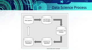
The document details an exploratory data analysis of 2017 US employment data using R, focusing on data sourced from the Bureau of Labor Statistics, encompassing 3.5 million rows. It illustrates the use of various R packages to visualize geographical distributions of wages and average employment levels across states and counties. The analysis includes data cleaning, merging, and visualization techniques to display average annual pay and jobs by industry.

1. Data Science
Exploratory data analysis
of 2017 US Employment data
using R – Use Case
Chetan Khanzode

2. Data Source
• Bureau of Labor Statistics (BLS)mission is the collection, analysis, and
dissemination of essential economic information to support public and
private decision-making.
• Data from Quarterly Census of Employment and Wages for year 2017
https://www.bls.gov/
• 3.5 million rows and 38 columns

3. Data Science Process
Source: data science cook book

4. R Packages Used
• library(data.table)
• library(plyr)
• library(dplyr)
• library(stringr)
• library(ggplot2)
• library(maps)
• library(bit64)
• library(RColorBrewer)
• library(choroplethr)

5. Import the data
Use fread function from the data.table package which is significantly faster

6. Merge the data with associated codes and Titles

7. Map package data
• Purpose is to look at the geographical distribution of
wages across the US.
• Map package has US map for both at the state-and
county-levels and the data required to make the
maps can be extracted.
• Then align our employment data with the map data
so that the correct data is represented at the right
location on the map.

8. Map package data

9. Map package data
state.fips$fips <- str_pad(state.fips$fips, width=2, pad="0“,side='left')

10. Map package data

11. Merge to main dataset
Merged data sample to main data frame

12. Geospatial data visualization
library(ggplot2)
library(RColorBrewer)
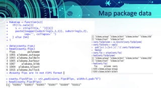
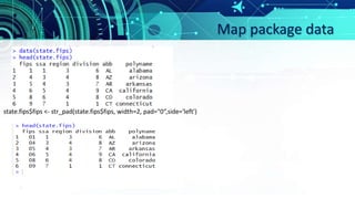
state_df <- map_data('state')
county_df <- map_data('county')
transform_mapdata <- function(x){
names(x)[5:6] <- c('state','county')
for(u in c('state','county')){
x[,u] <- sapply(x[,u],MakeCap)
}
return(x)
}
state_df <- transform_mapdata(state_df)
county_df <- transform_mapdata(county_df)
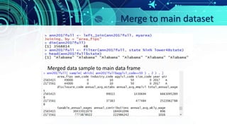
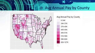
chor <- left_join(county_df, d.cty)
ggplot(chor, aes(long,lat, group=group))+
geom_polygon(aes(fill=wage))+
geom_path( color='white',alpha=0.5,size=0.2)+
geom_polygon(data=state_df, color='black',fill=NA)+
scale_fill_brewer(palette='PuRd')+
labs(x='',y='', fill='Avg Annual Pay by county')+
theme(axis.text.x=element_blank(), axis.text.y=element_blank(),
axis.ticks.x=element_blank(), axis.ticks.y=element_blank())
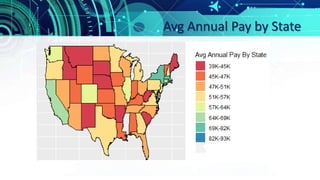
chor <- left_join(state_df, d.state)
ggplot(chor, aes(long,lat, group=group))+
geom_polygon(aes(fill=wage))+
geom_path( color='white',alpha=0.5,size=0.2)+
geom_polygon(data=state_df, color='black',fill=NA)+
scale_fill_brewer(palette='Spectral')+
labs(x='',y='', fill='Avg Annual Pay By State')+
theme(axis.text.x=element_blank(), axis.text.y=element_blank(),
axis.ticks.x=element_blank(), axis.ticks.y=element_blank())
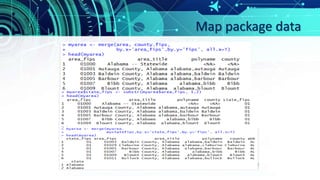
#The two functions filter and select are from dplyr.
d.cty <- filter(ann2017full, agglvl_code==70)%>%
select(state,county,abb, avg_annual_pay,
annual_avg_emplvl)%>%
mutate(wage=comDiscretize(avg_annual_pay),
empquantile=comDiscretize(annual_avg_emplvl))

13. Avg Annual Pay by County

14. Avg Annual Pay by State

15. JOBS by Industry - NIACS
d.sectors <- filter(ann2017full, industry_code %in%
c(11,21,54,52),
own_code==5, # Private sector
agglvl_code == 74 # county-level
) %>%
select(state,county,industry_code, own_code,agglvl_code,
industry_title, own_title, avg_annual_pay,
annual_avg_emplvl)%>%
mutate(wage=comDiscretize(avg_annual_pay),
emplevel=comDiscretize(annual_avg_emplvl))
d.sectors <- filter(d.sectors, !is.na(industry_code))
chor <- left_join(county_df, d.sectors)
ggplot(chor, aes(long,lat,group=group))+
geom_polygon(aes(fill=emplevel))+
geom_polygon(data=state_df, color='black',fill=NA)+
scale_fill_brewer(palette='PuBu')+
facet_wrap(~industry_title, ncol=2, as.table=T)+
labs(fill='Avg Employment Level',x='',y='')+
theme(axis.text.x=element_blank(),
axis.text.y=element_blank(),
axis.ticks.x=element_blank(),
axis.ticks.y=element_blank())

16. JOBS by Industry - NIACS

17. JOBS by Industry - NIACS

18. Thank You

19. References
https://www.bls.gov/
https://cran.r-project.org/web/packages/data.table/vignettes/datatable-intro.html
https://www.rdocumentation.org/packages/plyr/versions/1.8.4
https://cran.r-project.org/web/packages/dplyr/vignettes/dplyr.html
https://cran.r-project.org/web/packages/stringr/vignettes/stringr.html
https://www.statmethods.net/advgraphs/ggplot2.html
https://www.r-graph-gallery.com/map/
Practical data science book