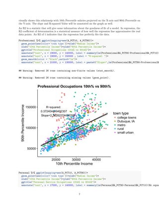
This document discusses an economic report for Iowa with a focus on Dubuque. Code is provided to import and organize labor data. Three main analyses are conducted: 1) An ANOVA test finds significant differences in median salaries between town types. 2) A chi-squared test finds no significant association between town type and occupation type. 3) A chi-squared test finds a highly significant association between occupation title and type.

1. Iowa Economic Report with Dubuque Focus
Michael Perhats
May 17, 2016
Necessary Code for the rest of the document to run:
#install.packages("readxl")
#install.packages(dplyr)
#install.packages("dplyr")
#install.packages("ggplot2")
#install.packages(cowplot)
#install.packages("gridExtra")
library(readxl)
## Warning: package 'readxl' was built under R version 3.2.5
library(dplyr)
## Warning: package 'dplyr' was built under R version 3.2.5
##
## Attaching package: 'dplyr'
## The following objects are masked from 'package:stats':
##
## filter, lag
## The following objects are masked from 'package:base':
##
## intersect, setdiff, setequal, union
library(ggplot2)
## Warning: package 'ggplot2' was built under R version 3.2.5
library(gridExtra)
## Warning: package 'gridExtra' was built under R version 3.2.5
##
## Attaching package: 'gridExtra'
## The following object is masked from 'package:dplyr':
##
## combine
1

2. library(cowplot)
## Warning: package 'cowplot' was built under R version 3.2.5
##
## Attaching package: 'cowplot'
## The following object is masked from 'package:ggplot2':
##
## ggsave
library(scales)
## Warning: package 'scales' was built under R version 3.2.5
Labor <- read_excel("C:/Users/mp518563/Documents/FINALE.xlsx")
tbl_df(Labor)
## Source: local data frame [2,635 x 17]
##
## AREA_NAME OCC_CODE
## (chr) (chr)
## 1 Ames, IA 11-0000
## 2 Ames, IA 13-0000
## 3 Ames, IA 15-0000
## 4 Ames, IA 17-0000
## 5 Ames, IA 19-0000
## 6 Ames, IA 21-0000
## 7 Ames, IA 23-0000
## 8 Ames, IA 25-0000
## 9 Ames, IA 27-0000
## 10 Ames, IA 29-0000
## .. ... ...
## Variables not shown: OCC_TITLE (chr), GROUP (chr), A_PCT10 (dbl), A_PCT25
## (dbl), A_MEDIAN (dbl), A_PCT75 (dbl), A_PCT90 (dbl), YEAR (time),
## Occupation Type (chr), total area emp for year (dbl), share of area
## employment (dbl), town type (chr), new occ title (chr), Total employment
## by town type (dbl), share of total employment by town type (dbl)
Labor<-tbl_df(Labor)
#ASSIGNING NAME TO DATA SET IN NEW TABLE FUCNTION
Labor %>% filter(`Occupation Type`=="Professional")
## Source: local data frame [1,078 x 17]
##
## AREA_NAME OCC_CODE
## (chr) (chr)
## 1 Ames, IA 11-0000
## 2 Ames, IA 13-0000
2

3. ## 3 Ames, IA 15-0000
## 4 Ames, IA 17-0000
## 5 Ames, IA 19-0000
## 6 Ames, IA 23-0000
## 7 Ames, IA 25-0000
## 8 Ames, IA 27-0000
## 9 Ames, IA 29-0000
## 10 Cedar Rapids, IA 11-0000
## .. ... ...
## Variables not shown: OCC_TITLE (chr), GROUP (chr), A_PCT10 (dbl), A_PCT25
## (dbl), A_MEDIAN (dbl), A_PCT75 (dbl), A_PCT90 (dbl), YEAR (time),
## Occupation Type (chr), total area emp for year (dbl), share of area
## employment (dbl), town type (chr), new occ title (chr), Total employment
## by town type (dbl), share of total employment by town type (dbl)
Professional <- Labor %>% filter(`Occupation Type`=="Professional")
Personal <- Labor %>% filter(`Occupation Type`=="Personal Services")
Manual <- Labor %>% filter(`Occupation Type`=="Mannual Labor")
#EXTRACTING FROM LABOR DATA SET, INFORMATION WHERE COLUMN HEADER EQUALS XYZ
rural <- Labor %>% filter(`town type`=="rural")
metro <- Labor %>% filter(`town type`=="metro")
college <- Labor %>% filter(`town type`=="college towns")
DBQ <- Labor %>% filter(`town type`=="Dubuque, IA")
small <- Labor %>% filter(`town type`=="small urban")
Introduction:
Our group studied and created visualizations for an “Economic report of Iowa with a focus on Dubuque.” We
got out data from the Bureau of Labor Statistics. As students in the state of Iowa for the next couple of
years, we wanted look for trends in the data in regards to the varying career fields that might provide us
with some generalized insight about trends in employment. Throughout our search for insight from the data
given, we noticed that there were some similar trends in the data in regards to the varying career fields that
might provide us with some generalized insight about trends in employment. In order to dive into this idea
in an accurate fashion we performed a principle components analysis with the salary data provided. When
we did this we found that the median salary was the principal component for analysis. We then proceeded to
use JMP’s clustering feature to cluster the occupation titles based on median salary. From this procedures
findings, we proceeded to collapse the 22 major Occupation Titles provided by the Bureau of Labor Statistics
into just 3 categories.
. Professional . Manual Labor . Personal Services This Process was performed in JMP (JMP is a SAS
product that is marketed as a ‘Statistical Discovery’ tool)
And, for geographical areas, collapsed 12 (the Bureau of Labor Statistics reports data for 12 separate regions
in Iowa) into 5.
These groupings permit a high level view of the Dubuque economy, how it has changed recently, and how it
compares with other areas of the state. Any of these analyses can be drilled down to a more disaggregated
level - but the reliability of the data will be reduced the more targeted the analysis (due to smaller sample
sizes).
1) Annova Test
The Null Hypothesis for our annova test is that there is no difference between Annual Median Salary and
Town Types (Dubuque, College Towns, Metro Areas, rural areas, and small urban areas) and that the means
3

4. and medians of attendance for all of these divisions are equivalent to one another. When Looking at the
results:
aov(Labor$A_MEDIAN~as.factor(Labor$`town type`))
## Call:
## aov(formula = Labor$A_MEDIAN ~ as.factor(Labor$`town type`))
##
## Terms:
## as.factor(Labor$`town type`) Residuals
## Sum of Squares 15973478269 588171751750
## Deg. of Freedom 4 2615
##
## Residual standard error: 14997.41
## Estimated effects may be unbalanced
## 15 observations deleted due to missingness
anova <- aov(Labor$A_MEDIAN~as.factor(Labor$`town type`))
summary(anova)
## Df Sum Sq Mean Sq F value Pr(>F)
## as.factor(Labor$`town type`) 4 1.597e+10 3.993e+09 17.75 2.17e-14 ***
## Residuals 2615 5.882e+11 2.249e+08
## ---
## Signif. codes: 0 '***' 0.001 '**' 0.01 '*' 0.05 '.' 0.1 ' ' 1
## 15 observations deleted due to missingness
Our p-value is less than 0.05. Hence we can conclude, for our confidence interval, the Alternative Hypothesis:
not all means are equal and that there is a relationship between town types and their median salaries. We
can also reject the null hypothesis that all of the means are the same and that there is no difference in annual
median salary between the town types.
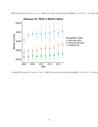
This can be depicted numerically with the following code, displaying the media
mean(DBQ$A_MEDIAN, na.rm = TRUE)
## [1] 36155.21
mean(college$A_MEDIAN, na.rm = TRUE)
## [1] 40332.53
mean(metro$A_MEDIAN, na.rm = TRUE)
## [1] 40374
mean(rural$A_MEDIAN, na.rm = TRUE)
## [1] 34782.75
4

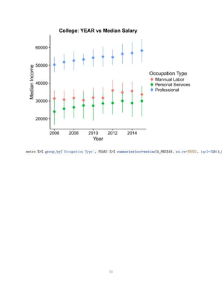
5. mean(small$A_MEDIAN, na.rm = TRUE)
## [1] 36794.75
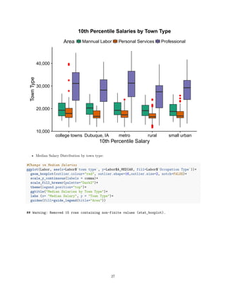
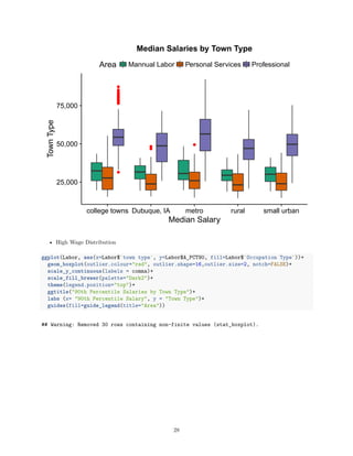
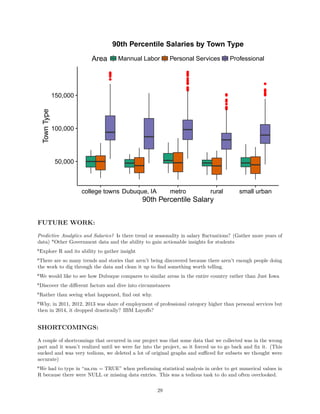
And Visually displayed with a box and whisker plot, showing the values as categorized by division:
ggplot(Labor, aes(x=Labor$`town type`, y=Labor$A_MEDIAN, fill=`town type`))+
geom_boxplot(outlier.colour="red", outlier.shape=16,outlier.size=2, notch=FALSE)+
coord_flip()+
scale_y_continuous(labels = comma)+
scale_fill_brewer(palette="Dark2")+
theme(legend.position="top")+
ggtitle("Attendance by LDiv")+
labs( x = "Median Salary", y = "Town Type")
## Warning: Removed 15 rows containing non-finite values (stat_boxplot).
college towns
Dubuque, IA
metro
rural
small urban
25,000 50,000 75,000
Town Type
MedianSalary
town type college towns Dubuque, IA metro rural small urban
Attendance by LDiv
*Note: College towns and metro areas seem to have higher annual median salaries as compared to the other
areas.
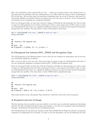
2) Chi-squared test between town type and occupation type
The Null hypothesis in the following chunk of code is that the two variables are independent and do not have
any statistically significant correlation.
5

6. Here, the calculated p-value exceeds 0.05, by a lot. . . which can be shown below in the chunk of code, so
the observation is consistent with the null hypothesis, as it falls within the range of what would happen
95% of the time. We can then reject the alternative hypothesis that we set out to discover, that there is a
statistically significant correlation between occupation type and town type in the Iowa. (I use a Chi-squared
test because we are comparing two categorical variables)
From our chi-squared table, we know that with the 8 degrees of freedom for this particular test, that in order
to reject our null hypothesis the test below would need to derive a value greater than 15.507 in order to reject
our Null hypothesis that there is no significant difference between our observed and expected frequencies
among these two variables. Our data shows a value of 0.03 which is much lower.
tbl <- table(Labor$`town type`, Labor$`Occupation Type`)
chisq.test(tbl)
##
## Pearson's Chi-squared test
##
## data: tbl
## X-squared = 0.026346, df = 8, p-value = 1
3) Chi-squared test between OCC_TITLE and Occupation Type
The Null hypothesis in the following chunk of code is that the two variables are independent and do not have
any statistically significant correlation.
Here, our chi p value is very very tiny. This means that we cannot accept our null hypothesis that there is
not any statistically significant correlation between OCC_TITLE and Occupation Type.
From our chi-squared table, we know that with the 40 degrees of freedom for this particular test, that in order
to reject our null hypothesis the test below would need to derive a value greater than 63.69 in order to reject
our Null hypothesis that there is no significant difference between our observed and expected frequencies
among these two variables. Our data shows a value of 5000 which is significantly high. . . .
tbl2 <- table(Labor$`OCC_TITLE`, Labor$`Occupation Type`)
chisq.test(tbl2)
##
## Pearson's Chi-squared test
##
## data: tbl2
## X-squared = 4944.2, df = 44, p-value < 2.2e-16
This makes intuitive sense, Occupation Type should be a reflection of the title of the occupation
4) R-squared and rate of change
The first question that we wanted to ask was whether or not there was a statistically significant relationship
between the 10th and 90th percentile wages and whether or not this was contingent upon Occupational
Category. (Professional, Personal Services and Manual Labor)
Our Null Hypothesis for this particular Analysis is that 10th and 90th Percent Wages for all three occupational
categories are independent of one another. In order to test this hypothesis, we run the following code that
6

7. visually shows this relationsip with 10th Percentile salaries projected on the X-axis and 90th Percentile on
the Y-axis. The slope and R-squared Value will be annotated on the graph as well.
An R2 is a statistic that will give some information about the goodness of fit of a model. In regression, the
R2 coefficient of determination is a statistical measure of how well the regression line approximates the real
data points. An R2 of 1 indicates that the regression line perfectly fits the data.
Professional %>% ggplot(mapping=aes(A_PCT10, A_PCT90))+
geom_point(aes(color=`town type`))+xlab("Median Income")+
xlab("10th Percentile Income")+ylab("90th Percentile Income")+
ggtitle("Professional Occupations 10th% vs 90th%")+
annotate("text", x = 19000, y = 140000, label = summary(lm(Professional$A_PCT90~Professional$A_PCT10))
annotate("text", x = 19000, y = 150000 , label = "R-squared: ")+
geom_smooth(color = "black",method="lm")+
annotate("text", x = 21000, y = 130000, label = paste0("Slope=",lm(Professional$A_PCT90~Professional$A
## Warning: Removed 26 rows containing non-finite values (stat_smooth).
## Warning: Removed 26 rows containing missing values (geom_point).
0.372404449492307
R−squared:
Slope=2.36282274458769
50000
100000
150000
20000 30000 40000
10th Percentile Income
90thPercentileIncome
town type
college towns
Dubuque, IA
metro
rural
small urban
Professional Occupations 10th% vs 90th%
Personal %>% ggplot(mapping=aes(A_PCT10, A_PCT90))+
geom_point(aes(color=`town type`))+xlab("Median Income")+
xlab("10th Percentile Income")+ylab("90th Percentile Income")+
ggtitle("Personal Service Occupations 10th% vs 90th%")+
annotate("text", x = 17000, y = 140000, label = summary(lm(Personal$A_PCT90~Personal$A_PCT10))$r.squar
7

8. annotate("text", x = 17000, y = 150000 , label = "R-squared: ")+
geom_smooth(color = "black",method="lm")+
annotate("text", x = 19000, y = 130000, label = paste0("Slope=",lm(Personal$A_PCT90~Personal$A_PCT10)$
## Warning: Removed 2 rows containing non-finite values (stat_smooth).
## Warning: Removed 2 rows containing missing values (geom_point).
0.194896906405275
R−squared:
Slope=2.41542651276843
40000
80000
120000
20000 30000 40000
10th Percentile Income
90thPercentileIncome
town type
college towns
Dubuque, IA
metro
rural
small urban
Personal Service Occupations 10th% vs 90th%
Manual %>% ggplot(mapping=aes(A_PCT10, A_PCT90))+
geom_point(aes(color=`town type`))+xlab("Median Income")+
xlab("10th Percentile Income")+ylab("90th Percentile Income")+
ggtitle("Manual Labor Occupations 10th% vs 90th%")+
annotate("text", x = 17000, y = 140000, label = summary(lm(Manual$A_PCT90~Manual$A_PCT10))$r.squared)+
annotate("text", x = 17000, y = 150000 , label = "R-squared: ")+
geom_smooth(color = "black",method="lm")+
annotate("text", x = 19000, y = 130000, label = paste0("Slope=",lm(Manual$A_PCT90~Manual$A_PCT10)$coef
## Warning: Removed 2 rows containing non-finite values (stat_smooth).
## Warning: Removed 2 rows containing missing values (geom_point).
8

9. 0.682938133320618
R−squared:
Slope=2.58596944563499
40000
80000
120000
16000 20000 24000
10th Percentile Income
90thPercentileIncome
town type
college towns
Dubuque, IA
metro
rural
small urban
Manual Labor Occupations 10th% vs 90th%
#storing code for the visualizations we want in new, easier to use variables
By the information provided by this visualization and the statistical analysis’ within, we can reject the Null
hypothesis that there is no connection between the two variables of comparison and accept the Alternative
Hypothesis that there is a connection between high wage earners and low wage earners salaries as predictors
of one another for each occupation provided by the BLS This being said, the correlation betweent the three
occupation types varies.
Highlights: * 10th Percentile salaries are fairly accurate predictors of the 90th percentile salaries for Manual
Labor Occupations * 10th Percentile Salaries are not accurate predictors of the 90th percentile salaries for
personal Services * for all three categories, the slope is fairly consistent at around 2.4.
5) Median Salary Fluctuations Over Time
The Following Visualization is a comparison of Median Salaries an dhow they have changed for each category
of occupation over the years.
For the professional category, there appears to be two groups: the college towns (Ames and Iowa City)
and the large metro areas are on one group, with the rest of the state (including Dubuque) having lower
professional salaries. Notable is the fact that professional salaries in Dubuque appear to have dropped since
2009, unlike the rest of the state. This would be something we might want to research to find reasons for.
Median incomes are highest for professional occupations, followed by the manual labor category, with personal
services the lowest in Dubuque. In the other categories, the median salaries were almost equivalent in the
last 10 years which is can be shown in the following figure
9

10. DBQ %>% group_by(`Occupation Type`, YEAR) %>% summarise(med=median(A_MEDIAN, na.rm=TRUE), iqr2=IQR(A_MED
20000
30000
40000
50000
60000
2006 2008 2010 2012 2014
Year
MedianIncome
Occupation Type
Mannual Labor
Personal Services
Professional
Dubuque, IA: YEAR vs Median Salary
college %>% group_by(`Occupation Type`, YEAR) %>% summarise(med=median(A_MEDIAN, na.rm=TRUE), iqr2=IQR(A
10

11. 20000
30000
40000
50000
60000
2006 2008 2010 2012 2014
Year
MedianIncome
Occupation Type
Mannual Labor
Personal Services
Professional
College: YEAR vs Median Salary
metro %>% group_by(`Occupation Type`, YEAR) %>% summarise(med=median(A_MEDIAN, na.rm=TRUE), iqr2=IQR(A_M
11

12. 20000
30000
40000
50000
60000
70000
2006 2008 2010 2012 2014
Year
MedianIncome
Occupation Type
Mannual Labor
Personal Services
Professional
Metro: YEAR vs Median Salary
small %>% group_by(`Occupation Type`, YEAR) %>% summarise(med=median(A_MEDIAN, na.rm=TRUE), iqr2=IQR(A_M
12

13. 20000
30000
40000
50000
60000
2006 2008 2010 2012 2014
Year
MedianIncome
Occupation Type
Mannual Labor
Personal Services
Professional
Small: YEAR vs Median Salary
rural %>% group_by(`Occupation Type`, YEAR) %>% summarise(med=median(A_MEDIAN, na.rm=TRUE), iqr2=IQR(A_M
13

14. 20000
30000
40000
50000
2006 2008 2010 2012 2014
Year
MedianIncome
Occupation Type
Mannual Labor
Personal Services
Professional
Rural: YEAR vs Median Salary
#TIME GRAPH VARIABLE ASSIGNMENTS
6) Share of Employment Dashboard
We thought that it would be advantageous to calculate what share of employment was held for each occupation
type. We did this with a simple formula, dividing the Total Employment number provided by the sum of the
Total employment across all categories for the year; leaving us with a percentage.
Using the same three occupational categories (Professional, Personal Services, Manual Labor) that we
calculated for the examples for the Dashboard representing the change in median salaries over time, we
have depicted what share of local employment falls into these three categories and how this ‘share’ has been
changing overtime.
Note that the share of employment that is “professional” has been rising throughout Iowa - in the college
towns and metro areas it has surpassed the share of employment in manual labor (which has been dropping
throughout the state).
DBQ %>% group_by(`Occupation Type`, YEAR) %>% summarise(med=median(`share of area employment`,na.rm=TRUE
14

15. 0.00
0.02
0.04
0.06
0.08
2006 2008 2010 2012 2014
Year
shareoftotalemploymentbytowntype,
Occupation Type
Mannual Labor
Personal Services
Professional
Dubuque, IA: YEAR vs share of total employment by town type
college %>% group_by(`Occupation Type`, YEAR) %>% summarise(med=median(`share of area employment`,na.rm=
15

16. 0.00
0.02
0.04
0.06
0.08
2006 2008 2010 2012 2014
Year
shareofareaemployment
Occupation Type
Mannual Labor
Personal Services
Professional
College: YEAR vs share of total employment by town type
metro %>% group_by(`Occupation Type`, YEAR) %>% summarise(med=median(`share of area employment`, na.rm=T
16

17. −0.025
0.000
0.025
0.050
0.075
2006 2008 2010 2012 2014
Year
shareofareaemployment
Occupation Type
Mannual Labor
Personal Services
Professional
Metro: YEAR vs share of total employment by town type
small %>% group_by(`Occupation Type`, YEAR) %>% summarise(med=median(`share of area employment`, na.rm=T
17

18. 0.000
0.025
0.050
0.075
2006 2008 2010 2012 2014
Year
shareofareaemployment
Occupation Type
Mannual Labor
Personal Services
Professional
Small: YEAR vs share of total employment by town type
rural %>% group_by(`Occupation Type`, YEAR) %>% summarise(med=median(`share of area employment`, na.rm=T
18

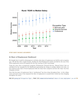
19. 0.00
0.02
0.04
0.06
0.08
2006 2008 2010 2012 2014
Year
shareofareaemployment
Occupation Type
Mannual Labor
Personal Services
Professional
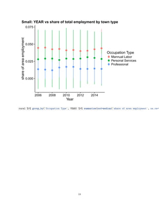
Rural: YEAR vs share of total employment by town type
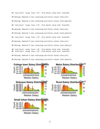
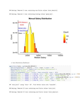
7) Histogram Distributions
A Histogram is diagram consisting of rectangles whose area is proportional to the frequency of a variable and
whose width is equal to the class interval.
• Center and Spread Statistics by town-
Dubuque:
sd(DBQ$A_MEDIAN, na.rm = TRUE)
## [1] 13975.85
median(DBQ$A_MEDIAN, na.rm = TRUE)
## [1] 32920
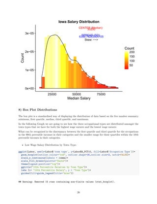
College Towns:
sd(college$A_MEDIAN, na.rm = TRUE)
## [1] 15748.84
19

20. median(college$A_MEDIAN, na.rm = TRUE)
## [1] 37985
Metro Areas:
sd(metro$A_MEDIAN, na.rm = TRUE)
## [1] 17485.75
median(metro$A_MEDIAN, na.rm = TRUE)
## [1] 36220
Rural Areas:
sd(rural$A_MEDIAN, na.rm = TRUE)
## [1] 12970.85
median(rural$A_MEDIAN, na.rm = TRUE)
## [1] 32400
Small Urban Areas:
sd(small$A_MEDIAN, na.rm = TRUE)
## [1] 14432.68
median(small$A_MEDIAN, na.rm = TRUE)
## [1] 34230
• College Towns have the highest annual median alary
• Rural towns have the lowest
• Dubuque is towards the lower end
• In regards to Salary remember, Dubuque also has less data points due to the lack of aggregation in this
category
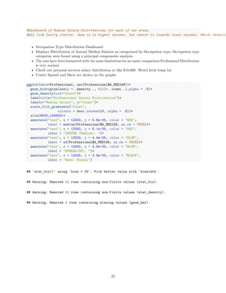
The visualization bellow depicts the statistics above (Town Type Distribution Dashboard):
DBQhist <- ggplot(data=DBQ, aes(DBQ$A_MEDIAN))+geom_histogram(aes(y =..density.., fill=..count..),alpha
Collegehist <- ggplot(data=college, aes(college$A_MEDIAN))+geom_histogram(aes(y =..density.., fill=..cou
Metrohist <- ggplot(data=metro, aes(metro$A_MEDIAN))+geom_histogram(aes(y =..density.., fill=..count..),
Smallhist <- ggplot(data=small, aes(small$A_MEDIAN))+geom_histogram(aes(y =..density.., fill=..count..),
Ruralhist <- ggplot(data=rural, aes(rural$A_MEDIAN))+geom_histogram(aes(y =..density.., fill=..count..),
grid.arrange (Collegehist, Metrohist, DBQhist, Smallhist, Ruralhist, ncol=2)
20

21. ## `stat_bin()` using `bins = 30`. Pick better value with `binwidth`.
## Warning: Removed 2 rows containing non-finite values (stat_bin).
## Warning: Removed 2 rows containing non-finite values (stat_density).
## `stat_bin()` using `bins = 30`. Pick better value with `binwidth`.
## Warning: Removed 2 rows containing non-finite values (stat_bin).
## Warning: Removed 2 rows containing non-finite values (stat_density).
## `stat_bin()` using `bins = 30`. Pick better value with `binwidth`.
## Warning: Removed 6 rows containing non-finite values (stat_bin).
## Warning: Removed 6 rows containing non-finite values (stat_density).
## `stat_bin()` using `bins = 30`. Pick better value with `binwidth`.
## `stat_bin()` using `bins = 30`. Pick better value with `binwidth`.
## Warning: Removed 5 rows containing non-finite values (stat_bin).
## Warning: Removed 5 rows containing non-finite values (stat_density).
0e+00
1e−05
2e−05
3e−05
250005000075000
Median Salary
Count
0
10
20
30
CountCollege town Salary Distribution
0e+00
1e−05
2e−05
3e−05
250005000075000
Median Salary
Count
10
20
30
40
50
CountMetro Salary Distribution
0e+00
1e−05
2e−05
3e−05
4e−05
5e−05
200004000060000
Median Salary
Count
0
5
10
15
20
CountDubuque Salary Distribution
0e+00
1e−05
2e−05
3e−05
200004000060000
Median Salary
Count
10
20
30
CountRural Salary Distribution
0e+00
1e−05
2e−05
3e−05
200004000060000
Median Salary
Count
20
40
60
CountSmall Urban Salary Distribution
21

22. #Dashboard of Median Salary Distributions for each of our areas.
#ALL look fairly similar, skew is to higher incomes, but center is towards lower incomes. Which intuitiv
• Occupation Type Distribution Dashboard
• Displays Distribution of Annual Median Salaries as categorized by Occupation type, Occupation type
categories were found using a principal components analysis.
• The axis have been formatted with the same limitations for an easier comparison Professional Distribution
is very normal.
• Check out personal services salary distribution at like $18,000. Weird little lump lol.
• Center Spread and Skew are shown on the graphs
ggplot(data=Professional, aes(Professional$A_MEDIAN))+
geom_histogram(aes(y =..density.., fill=..count..),alpha = .9)+
geom_density(col="black")+
labs(title="Professional Salary Distribution")+
labs(x="Median Salary", y="Count")+
scale_fill_gradientn("Count",
colours = heat.colors(16, alpha = .8))+
xlim(8000,100000)+
annotate("text", x = 12000, y = 5.6e-05, color = "RED",
label = median(Professional$A_MEDIAN, na.rm = TRUE))+
annotate("text", x = 12000, y = 6.1e-05, color = "RED",
label = "CENTER (Median): ")+
annotate("text", x = 12000, y = 4.4e-05, color = "BLUE",
label = sd(Professional$A_MEDIAN, na.rm = TRUE))+
annotate("text", x = 12000, y = 4.9e-05, color = "BLUE",
label = "SPREAD(SD): ")+
annotate("text", x = 12000, y = 3.9e-05, color = "BLACK",
label = "Skew: Normal")
## `stat_bin()` using `bins = 30`. Pick better value with `binwidth`.
## Warning: Removed 11 rows containing non-finite values (stat_bin).
## Warning: Removed 11 rows containing non-finite values (stat_density).
## Warning: Removed 1 rows containing missing values (geom_bar).
22

23. 50330
CENTER (Median):
13450.0891843386
SPREAD(SD):
Skew: Normal
0e+00
2e−05
4e−05
6e−05
25000 50000 75000 100000
Median Salary
Count
0
50
100
Count
Professional Salary Distribution
ggplot(data=Personal, aes(Personal$A_MEDIAN))+
geom_histogram(aes(y =..density.., fill=..count..),alpha = .9) +
geom_density(col="black")+
labs(title="Personal Services Salary Distribution")+
labs(x="Median Salary", y="Count")+
scale_fill_gradientn("Count",
colours = heat.colors(16, alpha = .8))+
xlim(8000,100000)+
annotate("text", x = 12000, y = 5.6e-05, color = "RED",
label = median(Personal$A_MEDIAN, na.rm = TRUE))+
annotate("text", x = 12000, y = 6.1e-05, color = "RED",
label = "CENTER (Median): ")+
annotate("text", x = 12000, y = 4.4e-05, color = "BLUE",
label = sd(Personal$A_MEDIAN, na.rm = TRUE))+
annotate("text", x = 12000, y = 4.9e-05, color = "BLUE",
label = "SPREAD(SD): ")+
annotate("text", x = 12000, y = 3.9e-05, color = "BLACK",
label = "Skew: -->")
## `stat_bin()` using `bins = 30`. Pick better value with `binwidth`.
## Warning: Removed 2 rows containing non-finite values (stat_bin).
## Warning: Removed 2 rows containing non-finite values (stat_density).
23

24. ## Warning: Removed 1 rows containing missing values (geom_bar).
24550
CENTER (Median):
7468.27680543114
SPREAD(SD):
Skew: −−>
0e+00
2e−05
4e−05
6e−05
25000 50000 75000 100000
Median Salary
Count
0
50
100
150
200
Count
Personal Services Salary Distribution
ggplot(data=Manual, aes(Manual$A_MEDIAN))+
geom_histogram(aes(y =..density.., fill=..count..),alpha = .9)+
geom_density(col="black")+
labs(title="Manual Salary Distribution") +
labs(x="Median Salary", y="Count")+
scale_fill_gradientn("Count",
colours = heat.colors(16, alpha = .8))+
xlim(8000,100000)+
annotate("text", x = 12000, y = 5.6e-05, color = "RED",
label = median(Manual$A_MEDIAN, na.rm = TRUE))+
annotate("text", x = 12000, y = 6.1e-05, color = "RED",
label = "CENTER (Median): ")+
annotate("text", x = 12000, y = 4.4e-05, color = "BLUE",
label = sd(Manual$A_MEDIAN, na.rm = TRUE))+
annotate("text", x = 12000, y = 4.9e-05, color = "BLUE",
label = "SPREAD (SD): ")+
annotate("text", x = 12000, y = 3.9e-05, color = "BLACK",
label = "Skew: -->")
## `stat_bin()` using `bins = 30`. Pick better value with `binwidth`.
## Warning: Removed 2 rows containing non-finite values (stat_bin).
24

25. ## Warning: Removed 2 rows containing non-finite values (stat_density).
## Warning: Removed 1 rows containing missing values (geom_bar).
30250
CENTER (Median):
6398.78263505105
SPREAD (SD):
Skew: −−>
0e+00
2e−05
4e−05
6e−05
25000 50000 75000 100000
Median Salary
Count
0
50
100
Count
Manual Salary Distribution
• Iowa Distribution Dashboard
ggplot(data=Labor, aes(Labor$A_MEDIAN))+
geom_histogram(aes(y =..density.., fill=..count..),alpha = .9)+
geom_density(col="black") +labs(title="Iowa Salary Distribution") +
labs(x="Median Salary", y="Count")+
scale_fill_gradientn("Count", colours = heat.colors(16, alpha = .8))+
annotate("text", x = 65000, y = 3.22e-05, color = "RED", label = median(Manual$A_MEDIAN, na.rm = TRUE)
annotate("text", x = 65000, y = 3.3e-05, color = "RED", label = "CENTER (Median): ")+
annotate("text", x = 65000, y = 2.82e-05, color = "BLUE", label = sd(Manual$A_MEDIAN, na.rm = TRUE))+
annotate("text", x = 65000, y = 2.9e-05, color = "BLUE", label = "SPREAD (SD): ")+
annotate("text", x = 65000, y = 2.65e-05, color = "BLACK", label = "Skew: -->")
## `stat_bin()` using `bins = 30`. Pick better value with `binwidth`.
## Warning: Removed 15 rows containing non-finite values (stat_bin).
## Warning: Removed 15 rows containing non-finite values (stat_density).
25

26. 30250
CENTER (Median):
6398.78263505105
SPREAD (SD):
Skew: −−>
0e+00
1e−05
2e−05
3e−05
25000 50000 75000
Median Salary
Count
50
100
150
200
Count
Iowa Salary Distribution
8) Box Plot Distributions
The box plot is a standardized way of displaying the distribution of data based on the five number summary:
minimum, first quartile, median, third quartile, and maximum.
In the following Graph we are going to see how the three occupational types are distributed amongst the
town types that we have for both the highest wage earners and the lowest wage earners
What can be recognized is the discrepancy between the first quartile and third quartile for the occupations
in the 90th percentile incomes in their categories and the smaller range for these quartiles within the 10th
percentile incomes in their categories.
• Low Wage Salary Distribution by Town Type:
ggplot(Labor, aes(x=Labor$`town type`, y=Labor$A_PCT10, fill=Labor$`Occupation Type`))+
geom_boxplot(outlier.colour="red", outlier.shape=16,outlier.size=2, notch=FALSE)+
scale_y_continuous(labels = comma)+
scale_fill_brewer(palette="Dark2")+
theme(legend.position="top")+
ggtitle("10th Percentile Salaries by Town Type")+
labs (x= "10th Percentile Salary", y = "Town Type")+
guides(fill=guide_legend(title="Area"))
## Warning: Removed 15 rows containing non-finite values (stat_boxplot).
26

27. 10,000
20,000
30,000
40,000
college towns Dubuque, IA metro rural small urban
10th Percentile Salary
TownType
Area Mannual Labor Personal Services Professional
10th Percentile Salaries by Town Type
• Median Salary Distribution by town type:
#Change in Median Salaries
ggplot(Labor, aes(x=Labor$`town type`, y=Labor$A_MEDIAN, fill=Labor$`Occupation Type`))+
geom_boxplot(outlier.colour="red", outlier.shape=16,outlier.size=2, notch=FALSE)+
scale_y_continuous(labels = comma)+
scale_fill_brewer(palette="Dark2")+
theme(legend.position="top")+
ggtitle("Median Salaries by Town Type")+
labs (x= "Median Salary", y = "Town Type")+
guides(fill=guide_legend(title="Area"))
## Warning: Removed 15 rows containing non-finite values (stat_boxplot).
27

28. 25,000
50,000
75,000
college towns Dubuque, IA metro rural small urban
Median Salary
TownType
Area Mannual Labor Personal Services Professional
Median Salaries by Town Type
• High Wage Distribution
ggplot(Labor, aes(x=Labor$`town type`, y=Labor$A_PCT90, fill=Labor$`Occupation Type`))+
geom_boxplot(outlier.colour="red", outlier.shape=16,outlier.size=2, notch=FALSE)+
scale_y_continuous(labels = comma)+
scale_fill_brewer(palette="Dark2")+
theme(legend.position="top")+
ggtitle("90th Percentile Salaries by Town Type")+
labs (x= "90th Percentile Salary", y = "Town Type")+
guides(fill=guide_legend(title="Area"))
## Warning: Removed 30 rows containing non-finite values (stat_boxplot).
28

29. 50,000
100,000
150,000
college towns Dubuque, IA metro rural small urban
90th Percentile Salary
TownType
Area Mannual Labor Personal Services Professional
90th Percentile Salaries by Town Type
FUTURE WORK:
Predictive Analytics and Salaries? Is there trend or seasonality in salary fluctuations? (Gather more years of
data) *Other Government data and the ability to gain actionable insights for students
*Explore R and its ability to gather insight
*There are so many trends and stories that aren’t being discovered because there aren’t enough people doing
the work to dig through the data and clean it up to find something worth telling.
*We would like to see how Dubuque compares to similar areas in the entire country rather than Just Iowa
*Discover the different factors and dive into circumstances
*Rather than seeing what happened, find out why.
*Why, in 2011, 2012, 2013 was share of employment of professional category higher than personal services but
then in 2014, it dropped drastically? IBM Layoffs?
SHORTCOMINGS:
A couple of shortcomings that occurred in our project was that some data that we collected was in the wrong
part and it wasn’t realized until we were far into the project, so it forced us to go back and fix it. (This
sucked and was very tedious, we deleted a lot of original graphs and sufficed for subsets we thought were
accurate)
*We had to type in “na.rm = TRUE” when performing statistical analysis in order to get numerical values in
R because there were NULL or missing data entries. This was a tedious task to do and often overlooked.
29

30. *Some of the data that they are starting to add, such as location quotient, in the newer BLs data is not
provided in the old data. This could have been a cool comparison
30