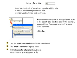
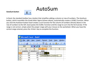
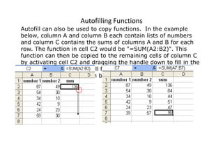
Presentation By- Manoj Jhawar, 12125027
Topics Covered…
•   MS Excel Topics
•   Ch-5 Using Formulas and Functions
•   Ch-6 Creating & Using Names
•   Ch-7 Auditing Your Work
•   Ch-8 Formatting Your Data
Formulas
Formulas are entered in the worksheet cell and must begin with an equal sign
"=". The formula then includes the addresses of the cells whose values will be
manipulated with appropriate operands placed in between. After the formula is
typed into the cell, the calculation executes immediately and the formula itself is
visible in the formula bar. See the example below to view the formula for
calculating the sub total for a number of textbooks. The formula multiplies the
quantity and price of each textbook and adds the subtotal for each book.
Formula Operators
 There are four basic Mathematical Operators when writing a formula. These operators are used to tell the
 formula what action to perform. The following table lists the operators, its symbol.

                                                Symbol
                   Operation                                 Symbol Name

                   Addition                        +         Plus Sign
                   Subtraction                     -         Dash or hyphen
                   Multiplication                  *         Asterisk
                   Division                        /         Forward slash

The next table lists the order of operation for each mathematical operator. As you begin to write your formulas,
keep in mind that information in parenthesis ( ) is always performed first while everything outside the
parenthesis is performed left to right.

            Operator               Operation                            Order of Calculation
            AND, OR, NOT           Logic Test: AND, OR, NOT             1
            + or -                 Positive or Negative Value           2
            ^                      Exponentiation                       3
            * or /                 Multiplication or Division           4
            +-                     Addition or Subtraction              5
            &                      Text Concatenation                   6
                                   Logic Test                           7
            =                      Equal to                             7
            <>                     Not Equal To                         7
            <=                     Less than or Equal to                7
            >=                     Greater than or Equal to             7
•
                                       Functions
          Built-in Excel Functions can be a faster way of doing mathematical operations than
          formulas.

•         Example- if you wanted to add the values of cells D1 through D10, you could type the
          formula "=D1+D2+D3+D4+D5+D6+D7+D8+D9+D10".

•         A shorter way would be to use the SUM function and simply type "=SUM(D1:D10)".


    Function      Example               Description
    SUM           =SUM(A1:A100)         finds the sum of cells A1 through A100
    AVERAGE       =AVERAGE(B1:B10)      finds the average of cells B1 through B10
    MAX           =MAX(C1:C100)         returns the highest number from cells C1 through C100
    MIN           =MIN(D1:D100)         returns the lowest number from cells D1 through D100
    SQRT          =SQRT(D10)            finds the square root of the value in cell D10
    TODAY         =TODAY()              returns the current date (leave the parentheses empty)


    SUM( ) function
    The SUM( ) function is probably the most common function in Excel. It adds a
    range of numbers. To build a SUM( ) function, begin by typing the = sign; all
    functions begin with the = sign. Next type the word SUM followed by an open
    parenthesis. You must now tell Excel which cells to sum. Using the mouse, click
    and drag over the range of cells you wish to add. A dotted outline will appear
    around the cells and the cell range will be displayed in the formula bar. When you
Insert Function
       Excel has hundreds of prewritten formulas which make
       it easy to do complex procedures with
       numbers, dates, times, text, and more.


                                   •Type a brief description of what you want to do
                                   in the Search for a function box. In this example,
                                   you could type "mortgage payment" or some
                                   other keywords.

                                   •Click Go.


Click the Insert Function button on the formula bar.
The Insert Function dialog box opens
In the Search for a function box, type a
description of what you want to do.
AutoSum button
                                       AutoSum
In Excel, the standard toolbar has a button that simplifies adding a column or row of numbers. The AutoSum
button, which resembles the Greek letter Sigma (shown above), automatically creates a SUM( ) function. When
you click the AutoSum button Excel creates a sum function for the column of numbers directly above or the
row of numbers to the left. Excel pastes the SUM( ) function and the range to sum into the formula bar. If the
range is not correct, simply select the proper range with your mouse on the worksheet. When you have the
correct range entered, press the <Enter> key to complete the function.
Autofilling Functions
Autofill can also be used to copy functions. In the example
below, column A and column B each contain lists of numbers
and column C contains the sums of columns A and B for each
row. The function in cell C2 would be "=SUM(A2:B2)". This
function can then be copied to the remaining cells of column C
by activating cell C2 and dragging the handle down to fill in the
remaining cells. The autofill feature will automatically update
the row numbers as shown below if the cells are reference
relatively
Names
To add borders around a
  cell or range, follow these
  steps:
   • 1. Select the cell or range.
   • 2. Click the arrow on the
     Borders button in the
     Ribbon’s Home tab. Excel
     displays the Borders menu.
   • 3. Choose a border style
     from the menu. Excel
     applies the border to your
     selection. In addition, the
     Borders button icon
     changes to reflect your
     border selection.
   Font Face: Select a font face from the font picker
    drop-down list.
   To preview the change in the selected cell or range
    before you commit to the
   change, hover the mouse pointer over a font face in
    the list.
    Font Size: Select a font size from the font picker
    drop-down list. To preview
   the change in the selected cell or range before you
    commit to the
   change, hover the mouse pointer over a font size in
    the list.
    Increase/Decrease Font Size: These buttons
    increase or decrease the
   font in the selected cell or range by 2 points.
    Font Style: The options are Bold, Italic and
    Underline. Click the arrow on
   the Underline button if you want to apply a double-
    underline to the contents
   of your selected cell or range.
   Hiding                            Unhiding
    • Select any cell(s) on the        • Select any cells on the
      worksheet in the column(s)           worksheets on either side of
      or row(s) that you want to           the column(s) or row(s) that
      hide. In the Ribbon’s Home           you want to unhide.For
      tab, choose                          example, if you want to
    • Format➪Hide &                    •   unhide columns E and
    • Unhide➪Hide Columns; or              F, select any row on the
      Format➪Hide &                        worksheet and select cells
      Unhide➪Hide Rows.                •   in columns D and G. In the
                                           Ribbon’s Home tab, choose
                                           Format➪Hide &
                                       •   Unhide➪Unhide Columns;
                                           or Format➪Hide &
                                           Unhide➪Unhide Rows.
                                       •    Select
Excel

Excel

  • 1.
    Presentation By- ManojJhawar, 12125027
  • 2.
    Topics Covered… • MS Excel Topics • Ch-5 Using Formulas and Functions • Ch-6 Creating & Using Names • Ch-7 Auditing Your Work • Ch-8 Formatting Your Data
  • 3.
    Formulas Formulas are enteredin the worksheet cell and must begin with an equal sign "=". The formula then includes the addresses of the cells whose values will be manipulated with appropriate operands placed in between. After the formula is typed into the cell, the calculation executes immediately and the formula itself is visible in the formula bar. See the example below to view the formula for calculating the sub total for a number of textbooks. The formula multiplies the quantity and price of each textbook and adds the subtotal for each book.
  • 4.
    Formula Operators Thereare four basic Mathematical Operators when writing a formula. These operators are used to tell the formula what action to perform. The following table lists the operators, its symbol. Symbol Operation Symbol Name Addition + Plus Sign Subtraction - Dash or hyphen Multiplication * Asterisk Division / Forward slash The next table lists the order of operation for each mathematical operator. As you begin to write your formulas, keep in mind that information in parenthesis ( ) is always performed first while everything outside the parenthesis is performed left to right. Operator Operation Order of Calculation AND, OR, NOT Logic Test: AND, OR, NOT 1 + or - Positive or Negative Value 2 ^ Exponentiation 3 * or / Multiplication or Division 4 +- Addition or Subtraction 5 & Text Concatenation 6 Logic Test 7 = Equal to 7 <> Not Equal To 7 <= Less than or Equal to 7 >= Greater than or Equal to 7
  • 5.
    Functions Built-in Excel Functions can be a faster way of doing mathematical operations than formulas. • Example- if you wanted to add the values of cells D1 through D10, you could type the formula "=D1+D2+D3+D4+D5+D6+D7+D8+D9+D10". • A shorter way would be to use the SUM function and simply type "=SUM(D1:D10)". Function Example Description SUM =SUM(A1:A100) finds the sum of cells A1 through A100 AVERAGE =AVERAGE(B1:B10) finds the average of cells B1 through B10 MAX =MAX(C1:C100) returns the highest number from cells C1 through C100 MIN =MIN(D1:D100) returns the lowest number from cells D1 through D100 SQRT =SQRT(D10) finds the square root of the value in cell D10 TODAY =TODAY() returns the current date (leave the parentheses empty) SUM( ) function The SUM( ) function is probably the most common function in Excel. It adds a range of numbers. To build a SUM( ) function, begin by typing the = sign; all functions begin with the = sign. Next type the word SUM followed by an open parenthesis. You must now tell Excel which cells to sum. Using the mouse, click and drag over the range of cells you wish to add. A dotted outline will appear around the cells and the cell range will be displayed in the formula bar. When you
  • 6.
    Insert Function Excel has hundreds of prewritten formulas which make it easy to do complex procedures with numbers, dates, times, text, and more. •Type a brief description of what you want to do in the Search for a function box. In this example, you could type "mortgage payment" or some other keywords. •Click Go. Click the Insert Function button on the formula bar. The Insert Function dialog box opens In the Search for a function box, type a description of what you want to do.
  • 7.
    AutoSum button AutoSum In Excel, the standard toolbar has a button that simplifies adding a column or row of numbers. The AutoSum button, which resembles the Greek letter Sigma (shown above), automatically creates a SUM( ) function. When you click the AutoSum button Excel creates a sum function for the column of numbers directly above or the row of numbers to the left. Excel pastes the SUM( ) function and the range to sum into the formula bar. If the range is not correct, simply select the proper range with your mouse on the worksheet. When you have the correct range entered, press the <Enter> key to complete the function.
  • 8.
    Autofilling Functions Autofill canalso be used to copy functions. In the example below, column A and column B each contain lists of numbers and column C contains the sums of columns A and B for each row. The function in cell C2 would be "=SUM(A2:B2)". This function can then be copied to the remaining cells of column C by activating cell C2 and dragging the handle down to fill in the remaining cells. The autofill feature will automatically update the row numbers as shown below if the cells are reference relatively
  • 9.
  • 10.
    To add bordersaround a cell or range, follow these steps: • 1. Select the cell or range. • 2. Click the arrow on the Borders button in the Ribbon’s Home tab. Excel displays the Borders menu. • 3. Choose a border style from the menu. Excel applies the border to your selection. In addition, the Borders button icon changes to reflect your border selection.
  • 11.
    Font Face: Select a font face from the font picker drop-down list.  To preview the change in the selected cell or range before you commit to the  change, hover the mouse pointer over a font face in the list.  Font Size: Select a font size from the font picker drop-down list. To preview  the change in the selected cell or range before you commit to the  change, hover the mouse pointer over a font size in the list.  Increase/Decrease Font Size: These buttons increase or decrease the  font in the selected cell or range by 2 points.  Font Style: The options are Bold, Italic and Underline. Click the arrow on  the Underline button if you want to apply a double- underline to the contents  of your selected cell or range.
  • 12.
    Hiding  Unhiding • Select any cell(s) on the • Select any cells on the worksheet in the column(s) worksheets on either side of or row(s) that you want to the column(s) or row(s) that hide. In the Ribbon’s Home you want to unhide.For tab, choose example, if you want to • Format➪Hide & • unhide columns E and • Unhide➪Hide Columns; or F, select any row on the Format➪Hide & worksheet and select cells Unhide➪Hide Rows. • in columns D and G. In the Ribbon’s Home tab, choose Format➪Hide & • Unhide➪Unhide Columns; or Format➪Hide & Unhide➪Unhide Rows. • Select