Error Estimates for Multi-Penalty Regularization under General Source Condition

Error Estimates for Multi-Penalty Regularization under
General Source Condition
Abhishake Rastogi
Department of Mathematics
Indian Institute of Technology Delhi
New Delhi 110016, India
abhishekrastogi2012@gmail.com
Abstract
In learning theory, the convergence issues of the regression problem are investigated with
the least square Tikhonov regularization schemes in both the RKHS-norm and the L 2
-norm.
We consider the multi-penalized least square regularization scheme under the general source
condition with the polynomial decay of the eigenvalues of the integral operator. One of the
motivation for this work is to discuss the convergence issues for widely considered manifold
regularization scheme. The optimal convergence rates of multi-penalty regularizer is achieved
in the interpolation norm using the concept of effective dimension. Further we also propose
the penalty balancing principle based on augmented Tikhonov regularization for the choice of
regularization parameters. The superiority of multi-penalty regularization over single-penalty
regularization is shown using the academic example and moon data set.
Keywords: Learning theory, Multi-penalty regularization, General source condition, Optimal
rates, Penalty balancing principle.
Mathematics Subject Classification 2010: 68T05, 68Q32.
1 Introduction
Let X be a compact metric space and Y ⊂ R with the joint probability measure ρ on Z = X×Y .
Suppose z = {(xi, yi)}m
i=1 ∈ Zm
be a observation set drawn from the unknown probability measure
ρ. The learning problem [1, 2, 3, 4] aims to approximate a function fz based on z such that
fz(x) ≈ y. We define the regression function fρ : X → Y by
fρ(x) :=
Y
ydρ(y|x) (1)
which is the minimizer of the generalization error
E(f) := Eρ(f) =
X Y
(f(x) − y)2
dρ(y|x)dρX(x). (2)
where ρ(y|x) and ρX(x) are conditional probability measure on Y and marginal probability measure
on X respectively. Therefore our objective becomes to estimate the regression function fρ.
Dhinaharan Nagamalai et al. (Eds) : AIS, CSIT, IPPR, IPDCA - 2017
pp. 201–216, 2017. c CS & IT-CSCP 2017 DOI : 10.5121/csit.2017.71016

202 Computer Science & Information Technology (CS & IT)
Single-penalty regularization is widely considered to infer the estimator from given set of ran-
dom samples [5, 6, 7, 8, 9, 10]. Smale et al. [9, 11, 12] provided the foundations of theoretical
analysis of square-loss regularization scheme under Hölder’s source condition. Caponnetto et al. [6]
improved the error estimates to optimal convergence rates for regularized least-square algorithm
using the polynomial decay condition of eigenvalues of the integral operator. But sometimes,
one may require to add more penalties to incorporate more features in the regularized solution.
Multi-penalty regularization is studied by various authors for both inverse problems and learning
algorithms [13, 14, 15, 16, 17, 18, 19, 20]. Belkin et al. [13] discussed the problem of manifold
regularization which controls the complexity of the function in ambient space as well as geometry
of the probability space:
f∗
= argmin
f∈HK



1
m
m
i=1
(f(xi) − yi)2
+ λA||f||2
HK
+ λI
n
i,j=1
(f(xi) − f(xj))2
ωij



, (3)
where {(xi, yi) ∈ X × Y : 1 ≤ i ≤ m} {xi ∈ X : m < i ≤ n} is given set of labeled and unlabeled
data, λA and λI are non-negative regularization parameters, ωij’s are non-negative weights, HK
is reproducing kernel Hilbert space and || · ||HK
is its norm.
Further, the manifold regularization algorithm is developed and widely considered in the vector-
valued framework to analyze the multi-task learning problem [21, 22, 23, 24] (Also see references
therein). So it motivates us to theoretically analyze this problem. The convergence issues of the
multi-penalty regularizer are discussed under general source condition in [25] but the convergence
rates are not optimal. Here we are able to achieve the optimal minimax convergence rates using
the polynomial decay condition of eigenvalues of the integral operator.
In order to optimize regularization functional, one of the crucial problem is the parameter
choice strategy. Various prior and posterior parameter choice rules are proposed for single-penalty
regularization [26, 27, 28, 29, 30] (also see references therein). Many regularization parameter se-
lection approaches are discussed for multi-penalized ill-posed inverse problems such as discrepancy
principle [15, 31], quasi-optimality principle [18, 32], balanced-discrepancy principle [33], heuristic
L-curve [34], noise structure based parameter choice rules [35, 36, 37], some approaches which
require reduction to single-penalty regularization [38]. Due to growing interest in multi-penalty
regularization in learning, multi-parameter choice rules are discussed in learning theory frame-
work such as discrepancy principle [15, 16], balanced-discrepancy principle [25], parameter choice
strategy based on generalized cross validation score [19]. Here we discuss the penalty balancing
principle (PB-principle) to choose the regularization parameters in our learning theory framework
which is considered for multi-penalty regularization in ill-posed problems [33].
1.1 Mathematical Preliminaries and Notations
Definition 1.1. Reproducing Kernel Hilbert Space (RKHS). For non-empty set X, the
real Hilbert space H of functions from X to Y is called reproducing kernel Hilbert space if for any
x ∈ X, the linear functional which maps f ∈ H to f(x) is continuous.
For each reproducing kernel Hilbert space H there exists a mercer kernel K : X × X → R such
that for Kx : X → R, defined as Kx(y) = K(x, y), the span of the set {Kx : x ∈ X} is dense in
H. Moreover, there is one to one correspondence between mercer kernels and reproducing kernel
Hilbert spaces [39]. So we denote the reproducing kernel Hilbert space H by HK corresponding to

Computer Science & Information Technology (CS & IT) 203
a mercer kernel K and its norm by || · ||K.
Definition 1.2. The sampling operator Sx : HK → Rm
associated with a discrete subset x =
{xi}m
i=1 is defined by
Sx(f) = (f(x))x∈x.
Then its adjoint is given by
S∗
xc =
1
m
m
i=1
ciKxi
, ∀c = (c1, · · · , cm) ∈ Rm
.
For each (xi, yi) ∈ Z, yi = fρ(xi) + ηxi
, where the probability distribution of ηxi
has mean 0 and
variance σ2
xi
. Denote σ2
:= 1
m
m
i=1
σ2
xi
< ∞ and κ := sup
x∈X
K(x, x) < ∞.
Learning Scheme. The optimization functional (3) can be expressed as
f∗
= argmin
f∈HK
||Sxf − y||2
m + λA||f||2
K + λI||(S∗
x LSx )1/2
f||2
K , (4)
where x = {xi ∈ X : 1 ≤ i ≤ n}, ||y||2
m = 1
m
m
i=1 y2
i , L = D − W with W = (ωij) is a weight
matrix with non-negative entries and D is a diagonal matrix with Dii =
n
j=1
ωij.
Here we consider a more general regularized learning scheme based on two penalties:
fz,λ := argmin
f∈HK
||Sxf − y||2
m + λ1||f||2
K + λ2||Bf||2
K , (5)
where B : HK → HK is a bounded operator and λ1, λ2 are non-negative parameters.
Theorem 1.1. If S∗
xSx + λ1I + λ2B∗
B is invertible, then the optimization functional (4) has
unique minimizer:
fz,λ = ∆SS∗
xy, where ∆S := (S∗
B)−1
.
We can obtain the explicit form of fz,λ by taking the functional derivative of the expression:
||Sxf − y||2
m + λ1||f||2
K + λ2||Bf||2
K= (S∗
B)f, f K − 2 S∗
xy, f K + ||y||2
m.
Define fx,λ as the minimizer of the optimization problem:
fx,λ := argmin
f∈HK
1
m
m
i=1
(f(xi) − fρ(xi))2
+ λ1||f||2
K + λ2||Bf||2
K (6)
which gives
fx,λ = ∆SS∗
xSxfρ. (7)
The data-free version of the considered regularization scheme (5) is
fλ := argmin
f∈HK
||f − fρ||2
ρ + λ1||f||2
K + λ2||Bf||2
K , (8)

where the norm || · ||ρ := || · ||L 2
ρX
. Then we get the expression of fλ,
fλ = (LK + λ1I + λ2B∗
B)−1
LKfρ (9)
and
fλ1
:= argmin
f∈HK
||f − fρ||2
ρ + λ1||f||2
K . (10)
which implies
fλ1
= (LK + λ1I)−1
LKfρ, (11)
where the integral operator LK : L 2
ρX
→ L 2
ρX
is a self-adjoint, non-negative, compact operator,
defined as
LK(f)(x) :=
X
K(x, t)f(t)dρX(t), x ∈ X.
The integral operator LK can also be defined as a self-adjoint operator on HK. We use the same
notation LK for both the operators.
Using the singular value decomposition LK =
∞
i=1
ti ·, ei Kei for orthonormal system {ei} in
HK and sequence of singular numbers κ2
≥ t1 ≥ t2 ≥ . . . ≥ 0, we define
φ(LK) =
∞
i=1
φ(ti) ·, ei Kei,
where φ is a continuous increasing index function defined on the interval [0, κ2
] with the assumption
φ(0) = 0.
We require some prior assumptions on the probability measure ρ to achieve the uniform con-
vergence rates for learning algorithms.
Assumption 1. (Source condition) Suppose
Ωφ,R := {f ∈ HK : f = φ(LK)g and ||g||K ≤ R} ,
Then the condition fρ ∈ Ωφ,R is usually referred as general source condition [40].
Assumption 2. (Polynomial decay condition) We assume the eigenvalues tn’s of the integral
operator LK follows the polynomial decay: For fixed positive constants α, β and b > 1,
αn−b
≤ tn ≤ βn−b
∀n ∈ N.
Following the notion of Bauer et al. [5] and Caponnetto et al. [6], we consider the class of
probability measures Pφ which satisfies the source condition and the probability measure class Pφ,b
satisfying the source condition and polynomial decay condition.
The effective dimension N(λ1) can be estimated from Proposition 3 [6] under the polynomial
decay condition as follows,
N(λ1) := Tr (LK + λ1I)−1
LK ≤
βb
b − 1
λ
−1/b
1 , for b > 1. (12)
where Tr(A) :=
∞
k=1
Aek, ek for some orthonormal basis {ek}∞
k=1.

Shuai Lu et al. [41] and Blanchard et al. [42] considered the logarithm decay condition of the
effective dimension N(λ1),
Assumption 3. (logarithmic decay) Assume that there exists some positive constant c > 0
such that
N(λ1) ≤ c log
1
λ1
, ∀λ1 > 0. (13)
2 Convergence Analysis
In this section, we discuss the convergence issues of multi-penalty regularization scheme on
reproducing kernel Hilbert space under the considered smoothness priors in learning theory frame-
work. We address the convergence rates of the multi-penalty regularizer by estimating the sample
error fz,λ − fλ and approximation error fλ − fρ in interpolation norm.
Proposition 2.1. Let z be i.i.d. samples drawn according to the probability measure ρ with the
hypothesis |yi| ≤ M for each (xi, yi) ∈ Z. Then for 0 ≤ s ≤ 1
2 and for every 0 < δ < 1 with prob.
1 − δ,
||Ls
K(fz,λ − fx,λ)||K ≤ 2λ
s− 1
2
1 Ξ 1 + 2 log
2
δ
+
4κM
3m
√
λ1
log
2
δ
,
where Nxi
(λ1) = Tr (LK + λ1I)−1
Kxi
K∗
xi
and Ξ = 1
m
m
i=1 σ2
xi
Nxi
(λ1) for the variance σ2
xi
of the probability distribution of ηxi
= yi − fρ(xi).
Proof. The expression fz,λ − fx,λ can be written as ∆SS∗
x(y − Sxfρ). Then we find that
||Ls
K(fz,λ − fx,λ)||K ≤ I1||Ls
K(LK + λ1I)−1/2
|| ||(LK + λ1I)1/2
∆S(LK + λ1I)1/2
||
≤ I1I2||Ls
K(LK + λ1I)−1/2
||, (14)
where I1 = ||(LK +λ1I)−1/2
S∗
x(y−Sxfρ)||K and I2 = ||(LK +λ1I)1/2
(S∗
xSx+λ1I)−1
(LK +λ1I)1/2
||.
For sufficiently large sample size m, the following inequality holds:
8κ2
√
m
log
2
δ
≤ λ1 (15)
Then from Theorem 2 [43] we have with confidence 1 − δ,
I3 = ||(LK + λ1I)−1/2
(LK − S∗
xSx)(LK + λ1I)−1/2
|| ≤
||S∗
xSx − LK||
λ1
≤
4κ2
√
mλ1
log
2
δ
≤
1
2
.
Then the Neumann series gives
I2 = ||{I − (LK + λ1I)−1/2
(LK − S∗
xSx)(LK + λ1I)−1/2
}−1
|| (16)
= ||
∞
i=0
{(LK + λ1I)−1/2
(LK − S∗
xSx)(LK + λ1I)−1/2
}i
|| ≤
∞
i=0
Ii
3 =
1
1 − I3
≤ 2.

Now we have,
||Ls
K(LK + λ1I)−1/2
|| ≤ sup
0<t≤κ2
ts
(t + λ1)1/2
≤ λ
s−1/2
1 for 0 ≤ s ≤
1
2
. (17)
To estimate the error bound for ||(LK + λ1I)−1/2
S∗
x(y − Sxfρ)||K using the McDiarmid inequality
(Lemma 2 [12]), deﬁne the function F : Rm
→ R as
F(y) = ||(LK + λ1I)−1/2
S∗
x(y − Sxfρ)||K
=
1
m
(LK + λ1I)−1/2
m
i=1
(yi − fρ(xi))Kxi
K
.
So F2
(y) = 1
m2
m
i,j=1
(yi − fρ(xi))(yj − fρ(xj)) (LK + λ1I)−1
Kxi
, Kxj K.
The independence of the samples together with Ey(yi − fρ(xi)) = 0, Ey(yi − fρ(xi))2
= σ2
xi
implies
Ey(F2
) =
1
m2
m
i=1
σ2
xi
Nxi
(λ1) ≤ Ξ2
,
where Nxi
(λ1) = Tr (LK + λ1I)−1
Kxi
K∗
xi
and Ξ = 1
m
m
i=1 σ2
xi
Nxi
(λ1). Since Ey(F) ≤
Ey(F2). It implies Ey(F) ≤ Ξ.
Let yi
= (y1, . . . , yi−1, yi, yi+1, . . . , ym), where yi is another sample at xi. We have
|F(y) − F(yi
)| ≤ ||(LK + λ1I)−1/2
S∗
x(y − yi
)||K
=
1
m
||(yi − yi)(LK + λ1I)−1/2
Kxi
||K ≤
2κM
m
√
λ1
.
This can be taken as B in Lemma 2(2) [12]. Now
Eyi |F(y) − Eyi (F(y))|2
≤
1
m2
Y Y
|yi − yi| ||(LK + λ1I)−1/2
Kxi
||Kdρ(yi|xi)
2
dρ(yi|xi)
≤
1
m2
Y Y
(yi − yi)
2
Nxi
(λ1)dρ(yi|xi)dρ(yi|xi)
≤
2
m2
σ2
xi
Nxi (λ1)
which implies
m
i=1
σ2
i (F) ≤ 2Ξ2
.
In view of Lemma 2(2) [12] for every ε > 0,
Prob
y∈Y m
{F(y) − Ey(F(y)) ≥ ε} ≤ exp −
ε2
4(Ξ2 + εκM/3m
√
λ1)
= δ. (let)
In terms of δ, probability inequality becomes
Prob
y∈Y m
F(y) ≤ Ξ 1 + 2 log
1
δ
+
4κM
3m
√
λ1
log
1
δ
≤ 1 − δ.
Incorporating this inequality with (16), (17) in (14), we get the desired result.

Proposition 2.2. Let z be i.i.d. samples drawn according to the probability measure ρ with the
hypothesis |yi| ≤ M for each (xi, yi) ∈ Z. Suppose fρ ∈ Ωφ,R. Then for 0 ≤ s ≤ 1
2 and for every
0 < δ < 1 with prob. 1 − δ,
||Ls
K(fz,λ − fλ)||K ≤
2λ
s− 1
2
1
√
m
3M N(λ1) +
4κ
√
λ1
||fλ − fρ||ρ +
√
λ1
6
||fλ − fρ||K
+
7κM
√
mλ1
log
4
δ
.
Proof. We can express fx,λ − fλ = ∆S(S∗
xSx − LK)(fρ − fλ), which implies
||Ls
K(fx,λ − fλ)||K ≤ I4
1
m
m
i=1
(fρ(xi) − fλ(xi))Kxi − LK(fρ − fλ)
K
.
where I4 = ||Ls
K∆S||. Using Lemma 3 [12] for the function fρ − fλ, we get with confidence 1 − δ,
||Ls
K(fx,λ − fλ)||K≤I4
4κ||fλ − fρ||∞
3m
log
1
δ
+
κ||fλ − fρ||ρ
√
m
1 + 8log
1
δ
. (18)
For sufficiently large sample (15), from Theorem 2 [43] we get
||(LK − S∗
xSx)(LK + λ1I)−1
|| ≤
||S∗
xSx − LK||
λ1
≤
4κ2
√
mλ1
log
2
δ
≤
1
2
with confidence 1 − δ, which implies
||(LK + λ1I)(S∗
xSx + λ1I)−1
|| = ||{I − (LK − S∗
xSx)(LK + λ1I)−1
}−1
|| ≤ 2. (19)
We have, ||Ls
K(LK + λ1I)−1
|| ≤ sup
0<t≤κ2
ts
(t + λ1)
≤ λs−1
1 for 0 ≤ s ≤ 1. (20)
Now equation (19) and (20) implies the following inequality,
I4≤||Ls
K(S∗
xSx + λ1I)−1
||≤||Ls
K(LK + λ1I)−1
|| ||(LK + λ1I)(S∗
xSx + λ1I)−1
||≤2λs−1
1 . (21)
Let ξ(x) = σ2
xNx(λ1) be the random variable. Then it satisfies |ξ| ≤ 4κ2
M2
/λ1, Ex(ξ) ≤ M2
N(λ1)
and σ2
(ξ) ≤ 4κ2
M4
N(λ1)/λ1. Using the Bernstein inequality we get
Prob
x∈Xm
m
i=1
σ2
xi
Nxi
(λ1) − M2
N(λ1) > t ≤ exp −
t2
/2
4mκ2M4N (λ1)
λ1
+ 4κ2M2t
3λ1
which implies
Prob
x∈Xm
Ξ ≤
M2N(λ1)
m
+
8κ2M2
3m2λ1
log
1
δ
≥ 1 − δ. (22)
We get the required error estimate by combining the estimates of Proposition 2.1 with inequalities
(18), (21), (22).
Proposition 2.3. Suppose fρ ∈ Ωφ,R. Then under the assumption that φ(t) and t1−s
/φ(t) are

nondecreasing functions, we have
||Ls
K(fλ − fρ)||K ≤ λs
1 Rφ(λ1) + λ2λ
−3/2
1 M||B∗
B|| . (23)
Proof. To realize the above error estimates, we decomposes fλ − fρ into fλ − fλ1
+ fλ1
− fρ. The
first term can be expressed as
fλ − fλ1
= −λ2(LK + λ1I + λ2B∗
B)−1
B∗
Bfλ1
.
Then we get
||Ls
K(fλ − fλ1
)||K ≤ λ2||Ls
K(LK + λ1I)−1
|| ||B∗
B|| ||fλ1
||K (24)
≤ λ2λs−1
1 ||B∗
B|| ||fλ1
||K ≤ λ2λ
s−3/2
1 M||B∗
B||.
||Ls
K(fλ1
− fρ)|| ≤ R||rλ1
(LK)Ls
Kφ(LK)|| ≤ Rλs
1φ(λ1), (25)
where rλ1 (t) = 1 − (t + λ1)−1
t.
Combining these error bounds, we achieve the required estimate.
Theorem 2.1. Let z be i.i.d. samples drawn according to probability measure Pφ,b. Suppose
φ(t) and t1−s
/φ(t) are nondecreasing functions. Then under parameter choice λ1 ∈ (0, 1], λ1 =
Ψ−1
(m−1/2
), λ2 = (Ψ−1
(m−1/2
))3/2
φ(Ψ−1
(m−1/2
)) where Ψ(t) = t
1
2 + 1
2b φ(t), for 0 ≤ s ≤ 1
2 and
for all 0 < δ < 1, the following error estimates holds with confidence 1 − δ,
Prob
z∈Zm
||Ls
K(fz,λ − fρ)||K ≤ C(Ψ−1
(m−1/2
))s
φ(Ψ−1
(m−1/2
)) log
4
δ
≥ 1 − δ,
where C = 14κM + (2 + 8κ)(R + M||B∗
B||) + 6M βb/(b − 1) and
lim
τ→∞
lim sup
m→∞
sup
ρ∈Pφ,b
Prob
z∈Zm
||Ls
K(fz,λ − fρ)||K > τ(Ψ−1
(m−1/2
))s
φ(Ψ−1
(m−1/2
)) =0.
Proof. Let Ψ(t) = t
1
2 + 1
2b φ(t). Then Ψ(t) = y follows,
lim
t→0
Ψ(t)
√
t
= lim
y→0
y
Ψ−1(y)
= 0.
Under the parameter choice λ1 = Ψ−1
(m−1/2
) we have lim
m→∞
mλ1 = ∞. Therefore for sufficiently
large m,
1
mλ1
=
λ
1
2b
1 φ(λ1)
√
mλ1
≤ λ
1
2b
1 φ(λ1).
Under the fact λ1 ≤ 1 from Proposition 2.2, 2.3 and eqn. (12) follows that with confidence 1 − δ,
||Ls
K(fz,λ − fρ)||K ≤ C(Ψ−1
(m−1/2
))s
φ(Ψ−1
(m−1/2
)) log
4
δ
, (26)
where C = 14κM + (2 + 8κ)(R + M||B∗
B||) + 6M βb/(b − 1).

Now defining τ := C log 4
δ gives δ = δτ = 4e−τ/C
. The estimate (26) can be reexpressed as
Prob
z∈Zm
{||Ls
K(fz,λ − fρ)||K > τ(Ψ−1
(m−1/2
))s
φ(Ψ−1
(m−1/2
))} ≤ δτ . (27)
Corollary 2.1. Under the same assumptions of Theorem 2.1 for Hölder’s source condition fρ ∈
Ωφ,R, φ(t) = tr
, for 0 ≤ s ≤ 1
2 and for all 0 < δ < 1, with confidence 1 − δ, for the parameter
choice λ1 = m− b
2br+b+1 and λ2 = m− 2br+3b
4br+2b+2 we have the following convergence rates:
||Ls
K(fz,λ − fρ)||K ≤ Cm−
b(r+s)
2br+b+1 log
4
δ
for 0 ≤ r ≤ 1 − s.
Corollary 2.2. Under the logarithm decay condition of effective dimension N(λ1), for Hölder’s
source condition fρ ∈ Ωφ,R, φ(t) = tr
, for 0 ≤ s ≤ 1
2 and for all 0 < δ < 1, with confidence
1 − δ, for the parameter choice λ1 = log m
m
1
2r+1
and λ2 = log m
m
2r+3
4r+2
we have the following
convergence rates:
||Ls
K(fz,λ − fρ)||K ≤ C
log m
m
s+r
2r+1
log
4
δ
for 0 ≤ r ≤ 1 − s.
Remark 2.1. The upper convergence rates of the regularized solution is estimated in the interpola-
tion norm for the parameter s ∈ [0, 1
2 ]. In particular, we obtain the error estimates in ||·||HK
-norm
for s = 0 and in || · ||L 2
ρX
-norm for s = 1
2 . We present the error estimates of multi-penalty
regularizer over the regularity class Pφ,b in Theorem 2.1 and Corollary 2.1. We can also obtain
the convergence rates of the estimator fz,λ under the source condition without the polynomial
decay of the eigenvalues of the integral operator LK by substituting N(λ1) ≤ κ2
λ1
. In addition,
for B = (S∗
x LSx )1/2
we obtain the error estimates of the manifold regularization scheme (29)
considered in [13].
Remark 2.2. The parameter choice is said to be optimal, if the minimax lower rates coincide with
the upper convergence rates for some λ = λ(m). For the parameter choice λ1 = Ψ−1
(m−1/2
) and
λ2 = (Ψ−1
(m−1/2
))3/2
φ(Ψ−1
(m−1/2
)), Theorem 2.1 share the upper convergence rates with the
lower convergence rates of Theorem 3.11, 3.12 [44]. Therefore the choice of parameters is optimal.
Remark 2.3. The results can be easily generalized to n-penalty regularization in vector-valued
framework. For simplicity, we discuss two-parameter regularization scheme in scalar-valued func-
tion setting.
Remark 2.4. We can also address the convergence issues of binary classification problem [45] using
our error estimates as similar to discussed in Section 3.3 [5] and Section 5 [9].
The proposed choice of parameters in Theorem 2.1 is based on the regularity parameters which
are generally not known in practice. In the proceeding section, we discuss the parameter choice
rules based on samples.
3 Parameter Choice Rules
Most regularized learning algorithms depend on the tuning parameter, whose appropriate choice
is crucial to ensure good performance of the regularized solution. Many parameter choice strategies

are discussed for single-penalty regularization schemes for both ill-posed problems and the learning
algorithms [27, 28] (also see references therein). Various parameter choice rules are studied for
multi-penalty regularization schemes [15, 18, 19, 25, 31, 32, 33, 36, 46]. Ito el al. [33] studied
a balancing principle for choosing regularization parameters based on the augmented Tikhonov
regularization approach for ill posed inverse problems. In learning theory framework, we are
discussing the fixed point algorithm based on the penalty balancing principle considered in [33].
The Bayesian inference approach provides a mechanism for selecting the regularization parame-
ters through hierarchical modeling. Various authors successfully applied this approach in different
problems. Thompson et al. [47] applied this for selecting parameters for image restoration. Jin et
al. [48] considered the approach for ill-posed Cauchy problem of steady-state heat conduction.
The posterior probability density function (PPDF) for the functional (4) is given by
P(f, σ2
, µ, z) ∝
1
σ2
n/2
exp −
1
2σ2
||Sxf − y||2
m µ
n1/2
1 exp −
µ1
2
||f||2
K µ
n2/2
2
· exp −
µ2
2
||Bf||2
K µα −1
1 e−β µ1
µα −1
2 e−β µ2
1
σ2
αo−1
e−βo( 1
σ2 )
.
where (α , β ) are parameter pairs for µ = (µ1, µ2), (αo, βo) are parameter pair for inverse variance
1
σ2 . In the Bayesian inference approach, we select parameter set (f, σ2
, µ) which maximizes the
PPDF. By taking the negative logarithm and simplifying, the problem can be reformulated as
J (f, τ, µ) = τ||Sxf − y||2
m + µ1||f||2
K + µ2||Bf||2
K
+β(µ1 + µ2) − α(logµ1 + logµ2) + βoτ − αologτ,
where τ = 1/σ2
, β = 2β , α = n1 + 2α − 2, βo = 2βo, αo = n2 + 2αo − 2. We assume that
the scalars τ and µi’s have Gamma distributions with known parameter pairs. The functional is
pronounced as augmented Tikhonov regularization.
For non-informative prior βo = β = 0, the optimality of a-Tikhonov functional can be reduced to



fz,λ = arg min
f∈HK
||Sxf − y||2
m + λ1||f||2
K + λ2||Bf||2
K
µ1 = α
||fz,λ||2
K
, µ2 = α
||Bfz,λ||2
K
τ = αo
||Sxfz,λ−y||2
m
where λ1 = µ1
τ , λ2 = µ2
τ , γ = αo
α , this can be reformulated as



fz,λ = arg min
f∈HK
||Sxf − y||2
m + λ1||f||2
K + λ2||Bf||2
K
λ1 = 1
γ
||Sxfz,λ−y||2
m
||fz,λ||2
K
, λ2 = 1
γ
||Sxfz,λ−y||2
m
||Bfz,λ||2
K
which implies
λ1||fz,λ||2
K = λ2||Bfz,λ||2
K.
It selects the regularization parameter λ in the functional (5) by balancing the penalty with
the fidelity. Therefore the term “Penalty balancing principle” follows. Now we describe the fixed
point algorithm based on PB-principle.

Algorithm 1 Parameter choice rule “Penalty-balancing Principle”
1. For an initial value λ = (λ0
1, λ0
2), start with k = 0.
2. Calculate fz,λk and update λ by
λk+1
1 =
||Sxfz,λk − y||2
m + λk
2||Bfz,λk ||2
K
(1 + γ)||fz,λk ||2
K
,
λk+1
2 =
||Sxfz,λk − y||2
m + λk
1||fz,λk ||2
K
(1 + γ)||Bfz,λk ||2
K
.
3. If stopping criteria ||λk+1
− λk
|| < ε satisﬁed then stop otherwise set k = k + 1 and GOTO
(2).
4 Numerical Realization
In this section, the performance of single-penalty regularization versus multi-penalty regular-
ization is demonstrated using the academic example and two moon data set. For single-penalty
regularization, parameters are chosen according to the quasi-optimality principle while for two-
parameter regularization according to PB-principle.
We consider the well-known academic example [28, 16, 49] to test the multi-penalty regulariza-
tion under PB-principle parameter choice rule,
fρ(x) =
1
10
x + 2 e−8( 4π
3 −x)2
− e−8( π
2 −x)2
− e−8( 3π
2 −x)2
, x ∈ [0, 2π], (28)
which belongs to reproducing kernel Hilbert space HK corresponding to the kernel K(x, y) =
xy +exp (−8(x − y)2
). We generate noisy data 100 times in the form y = fρ(x)+δξ corresponding
to the inputs x = {xi}m
i=1 = { π
10 (i − 1)}m
i=1, where ξ follows the uniform distribution over [−1, 1]
with δ = 0.02.
We consider the following multi-penalty functional proposed in the manifold regularization
[13, 15],
argmin
f∈HK
1
m
m
i=1
(f(xi) − yi)2
+ λ1||f||2
K + λ2||(S∗
x LSx )1/2
f||2
K , (29)
where x = {xi ∈ X : 1 ≤ i ≤ n} and L = D − W with W = (ωij) is a weight matrix with
non-negative entries and D is a diagonal matrix with Dii =
n
j=1
ωij.
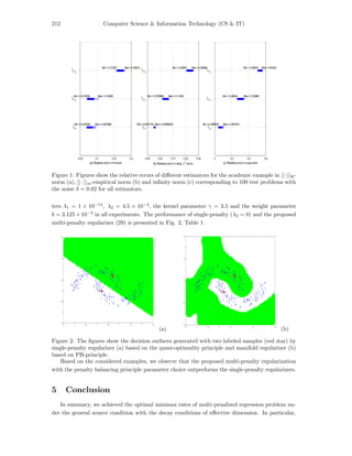
In our experiment, we illustrate the error estimates of single-penalty regularizers f = fz,λ1
,
f = fz,λ2
and multi-penalty regularizer f = fz,λ using the relative error measure
||f−fρ||
||f|| for the
academic example in sup norm, HK-norm and || · ||m-empirical norm in Fig. 1 (a), (b) & (c)
respectively.
Now we compare the performance of multi-penalty regularization over single-penalty regular-
ization method using the well-known two moon data set (Fig. 2) in the context of manifold
learning. The data set contains 200 examples with k labeled example for each class. We perform
experiments 500 times by taking l = 2k = 2, 6, 10, 20 labeled points randomly. We solve the man-
ifold regularization problem (29) for the mercer kernel K(xi, xj) = exp(−γ||xi − xj||2
) with the
exponential weights ωij = exp(−||xi − xj||2
/4b), for some b, γ > 0. We choose initial parame-

Figure 1: Figures show the relative errors of different estimators for the academic example in ||·||H-
norm (a), || · ||m-empirical norm (b) and infinity norm (c) corresponding to 100 test problems with
the noise δ = 0.02 for all estimators.
ters λ1 = 1 × 10−14
, λ2 = 4.5 × 10−3
, the kernel parameter γ = 3.5 and the weight parameter
b = 3.125 × 10−3
in all experiments. The performance of single-penalty (λ2 = 0) and the proposed
multi-penalty regularizer (29) is presented in Fig. 2, Table 1.
(a) (b)
Figure 2: The figures show the decision surfaces generated with two labeled samples (red star) by
single-penalty regularizer (a) based on the quasi-optimality principle and manifold regularizer (b)
based on PB-principle.
Based on the considered examples, we observe that the proposed multi-penalty regularization
with the penalty balancing principle parameter choice outperforms the single-penalty regularizers.
5 Conclusion
In summary, we achieved the optimal minimax rates of multi-penalized regression problem un-
der the general source condition with the decay conditions of effective dimension. In particular,

Single-penalty Regularizer Multi-penalty Regularizer
(SP %) (WC) Parameters (SP %) (WC) Parameters
m = 2 76.984 89 λ1 = 1.2 × 10−14
100 0 λ1 = 1.1103 × 10−14
λ2 = 5.9874 × 10−4
m = 6 88.249 112 λ1 = 1.2 × 10−14
100 0 λ1 = 9.8784 × 10−15
λ2 = 5.7020 × 10−4
m = 10 93.725 77 λ1 = 1.2 × 10−14
100 0 λ1 = 1.0504 × 10−14
λ2 = 7.3798 × 10−4
m = 20 98.100 40 λ1 = 1.2 × 10−14
100 0 λ1 = 1.0782 × 10−14
λ2 = 7.0076 × 10−4
Table 1: Statistical performance interpretation of single-penalty (λ2 = 0) and multi-penalty regu-
larizers of the functional
Symbols: labeled points (m); successfully predicted (SP); maximum of wrongly classified points
(WC)
the convergence analysis of multi-penalty regularization provide the error estimates of manifold
regularization problem. We can also address the convergence issues of binary classification problem
using our error estimates. Here we discussed the penalty balancing principle based on augmented
Tikhonov regularization for the choice of regularization parameters. Many other parameter choice
rules are proposed to obtain the regularized solution of multi-parameter regularization schemes.
The next problem of interest can be the rigorous analysis of different parameter choice rules of
multi-penalty regularization schemes. Finally, the superiority of multi-penalty regularization over
single-penalty regularization is shown using the academic example and moon data set.
Acknowledgements: The authors are grateful for the valuable suggestions and comments of
the anonymous referees that led to improve the quality of the paper.
References
[1] O. Bousquet, S. Boucheron, and G. Lugosi, “Introduction to statistical learning theory,” in
Advanced lectures on machine learning, pp. 169–207, Berlin/Heidelberg: Springer, 2004.
[2] F. Cucker and S. Smale, “On the mathematical foundations of learning,” Bull. Amer. Math.
Soc. (NS), vol. 39, no. 1, pp. 1–49, 2002.
[3] T. Evgeniou, M. Pontil, and T. Poggio, “Regularization networks and support vector ma-
chines,” Adv. Comput. Math., vol. 13, no. 1, pp. 1–50, 2000.
[4] V. N. Vapnik and V. Vapnik, Statistical Learning Theory, vol. 1. New York: Wiley, 1998.
[5] F. Bauer, S. Pereverzev, and L. Rosasco, “On regularization algorithms in learning theory,”
J. Complexity, vol. 23, no. 1, pp. 52–72, 2007.
[6] A. Caponnetto and E. De Vito, “Optimal rates for the regularized least-squares algorithm,”
Found. Comput. Math., vol. 7, no. 3, pp. 331–368, 2007.
[7] H. W. Engl, M. Hanke, and A. Neubauer, Regularization of Inverse Problems, vol. 375. Dor-
drecht, The Netherlands: Math. Appl., Kluwer Academic Publishers Group, 1996.

[8] L. L. Gerfo, L. Rosasco, F. Odone, E. De Vito, and A. Verri, “Spectral algorithms for super-
vised learning,” Neural Computation, vol. 20, no. 7, pp. 1873–1897, 2008.
[9] S. Smale and D. X. Zhou, “Learning theory estimates via integral operators and their approx-
imations,” Constr. Approx., vol. 26, no. 2, pp. 153–172, 2007.
[10] A. N. Tikhonov and V. Y. Arsenin, Solutions of Ill-posed Problems, vol. 14. Washington, DC:
W. H. Winston, 1977.
[11] S. Smale and D. X. Zhou, “Shannon sampling and function reconstruction from point values,”
Bull. Amer. Math. Soc., vol. 41, no. 3, pp. 279–306, 2004.
[12] S. Smale and D. X. Zhou, “Shannon sampling II: Connections to learning theory,” Appl.
Comput. Harmonic Anal., vol. 19, no. 3, pp. 285–302, 2005.
[13] M. Belkin, P. Niyogi, and V. Sindhwani, “Manifold regularization: A geometric framework for
learning from labeled and unlabeled examples,” J. Mach. Learn. Res., vol. 7, pp. 2399–2434,
2006.
[14] D. Düvelmeyer and B. Hofmann, “A multi-parameter regularization approach for estimating
parameters in jump diffusion processes,” J. Inverse Ill-Posed Probl., vol. 14, no. 9, pp. 861–
880, 2006.
[15] S. Lu and S. V. Pereverzev, “Multi-parameter regularization and its numerical realization,”
Numer. Math., vol. 118, no. 1, pp. 1–31, 2011.
[16] S. Lu, S. Pereverzyev Jr., and S. Sivananthan, “Multiparameter regularization for construction
of extrapolating estimators in statistical learning theory,” in Multiscale Signal Analysis and
Modeling, pp. 347–366, New York: Springer, 2013.
[17] Y. Lu, L. Shen, and Y. Xu, “Multi-parameter regularization methods for high-resolution
image reconstruction with displacement errors,” IEEE Trans. Circuits Syst. I: Regular Papers,
vol. 54, no. 8, pp. 1788–1799, 2007.
[18] V. Naumova and S. V. Pereverzyev, “Multi-penalty regularization with a component-wise
penalization,” Inverse Problems, vol. 29, no. 7, p. 075002, 2013.
[19] S. N. Wood, “Modelling and smoothing parameter estimation with multiple quadratic penal-
ties,” J. R. Statist. Soc., vol. 62, pp. 413–428, 2000.
[20] P. Xu, Y. Fukuda, and Y. Liu, “Multiple parameter regularization: Numerical solutions and
applications to the determination of geopotential from precise satellite orbits,” J. Geodesy,
vol. 80, no. 1, pp. 17–27, 2006.
[21] Y. Luo, D. Tao, C. Xu, D. Li, and C. Xu, “Vector-valued multi-view semi-supervsed learning
for multi-label image classification.,” in AAAI, pp. 647–653, 2013.
[22] Y. Luo, D. Tao, C. Xu, C. Xu, H. Liu, and Y. Wen, “Multiview vector-valued manifold
regularization for multilabel image classification,” IEEE Trans. Neural Netw. Learn. Syst.,
vol. 24, no. 5, pp. 709–722, 2013.

[23] H. Q. Minh, L. Bazzani, and V. Murino, “A unifying framework in vector-valued reproducing
kernel Hilbert spaces for manifold regularization and co-regularized multi-view learning,” J.
Mach. Learn. Res., vol. 17, no. 25, pp. 1–72, 2016.
[24] H. Q. Minh and V. Sindhwani, “Vector-valued manifold regularization,” in International Con-
ference on Machine Learning, 2011.
[25] Abhishake and S. Sivananthan, “Multi-penalty regularization in learning theory,” J. Com-
plexity, vol. 36, pp. 141–165, 2016.
[26] F. Bauer and S. Kindermann, “The quasi-optimality criterion for classical inverse problems,”
Inverse Problems, vol. 24, p. 035002, 2008.
[27] A. Caponnetto and Y. Yao, “Cross-validation based adaptation for regularization operators
in learning theory,” Anal. Appl., vol. 8, no. 2, pp. 161–183, 2010.
[28] E. De Vito, S. Pereverzyev, and L. Rosasco, “Adaptive kernel methods using the balancing
principle,” Found. Comput. Math., vol. 10, no. 4, pp. 455–479, 2010.
[29] V. A. Morozov, “On the solution of functional equations by the method of regularization,”
Soviet Math. Dokl, vol. 7, no. 1, pp. 414–417, 1966.
[30] J. Xie and J. Zou, “An improved model function method for choosing regularization parame-
ters in linear inverse problems,” Inverse Problems, vol. 18, no. 3, pp. 631–643, 2002.
[31] S. Lu, S. V. Pereverzev, and U. Tautenhahn, “A model function method in regularized total
least squares,” Appl. Anal., vol. 89, no. 11, pp. 1693–1703, 2010.
[32] M. Fornasier, V. Naumova, and S. V. Pereverzyev, “Parameter choice strategies for multi-
penalty regularization,” SIAM J. Numer. Anal., vol. 52, no. 4, pp. 1770–1794, 2014.
[33] K. Ito, B. Jin, and T. Takeuchi, “Multi-parameter Tikhonov regularization–An augmented
approach,” Chinese Ann. Math., vol. 35, no. 3, pp. 383–398, 2014.
[34] M. Belge, M. E. Kilmer, and E. L. Miller, “Eﬃcient determination of multiple regularization
parameters in a generalized L-curve framework,” Inverse Problems, vol. 18, pp. 1161–1183,
2002.
[35] F. Bauer and O. Ivanyshyn, “Optimal regularization with two interdependent regularization
parameters,” Inverse problems, vol. 23, no. 1, pp. 331–342, 2007.
[36] F. Bauer and S. V. Pereverzev, “An utilization of a rough approximation of a noise covariance
within the framework of multi-parameter regularization,” Int. J. Tomogr. Stat, vol. 4, pp. 1–
12, 2006.
[37] Z. Chen, Y. Lu, Y. Xu, and H. Yang, “Multi-parameter Tikhonov regularization for linear
ill-posed operator equations,” J. Comp. Math., vol. 26, pp. 37–55, 2008.
[38] C. Brezinski, M. Redivo-Zaglia, G. Rodriguez, and S. Seatzu, “Multi-parameter regularization
techniques for ill-conditioned linear systems,” Numer. Math., vol. 94, no. 2, pp. 203–228, 2003.
[39] N. Aronszajn, “Theory of reproducing kernels,” Trans. Amer. Math. Soc., vol. 68, pp. 337–404,
1950.

[40] P. Mathé and S. V. Pereverzev, “Geometry of linear ill-posed problems in variable Hilbert
scales,” Inverse problems, vol. 19, no. 3, pp. 789–803, 2003.
[41] S. Lu, P. Mathé, and S. Pereverzyev, “Balancing principle in supervised learning for a general
regularization scheme,” RICAM-Report, vol. 38, 2016.
[42] G. Blanchard and P. Mathé, “Discrepancy principle for statistical inverse problems with ap-
plication to conjugate gradient iteration,” Inverse problems, vol. 28, no. 11, p. 115011, 2012.
[43] E. De Vito, L. Rosasco, A. Caponnetto, U. De Giovannini, and F. Odone, “Learning from
examples as an inverse problem,” J. Mach. Learn. Res., vol. 6, pp. 883–904, 2005.
[44] A. Rastogi and S. Sivananthan, “Optimal rates for the regularized learning algorithms under
general source condition,” Front. Appl. Math. Stat., vol. 3, p. 3, 2017.
[45] S. Boucheron, O. Bousquet, and G. Lugosi, “Theory of classification: A survey of some recent
advances,” ESAIM: probability and statistics, vol. 9, pp. 323–375, 2005.
[46] S. Lu and S. Pereverzev, Regularization Theory for Ill-posed Problems: Selected Topics, vol. 58.
Berlin: Walter de Gruyter, 2013.
[47] A. M. Thompson and J. Kay, “On some choices of regularization parameter in image restora-
tion,” Inverse Problems, vol. 9, pp. 749–761, 1993.
[48] B. Jin and J. Zou, “Augmented Tikhonov regularization,” Inverse Problems, vol. 25, no. 2,
p. 025001, 2008.
[49] C. A. Micchelli and M. Pontil, “Learning the kernel function via regularization,” J. Mach.
Learn. Res., vol. 6, no. 2, pp. 1099–1125, 2005.

Error Estimates for Multi-Penalty Regularization under General Source Condition

Recommended

Recommended

More Related Content

What's hot

What's hot (20)

Similar to Error Estimates for Multi-Penalty Regularization under General Source Condition

Similar to Error Estimates for Multi-Penalty Regularization under General Source Condition (20)

Recently uploaded

Recently uploaded (20)

Error Estimates for Multi-Penalty Regularization under General Source Condition