Downloaded 10 times


![List of Tables
1.1 Some two-dimensional Poisson solvers with arithmetic complexity
[92]. N is the number of unknowns . . . . . . . . . . . . . . . . . 11
2.1 Number of grid points employed, related to the wavenumber, so
that kh = 0.625. . . . . . . . . . . . . . . . . . . . . . . . . . . . 20
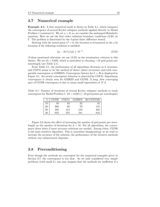
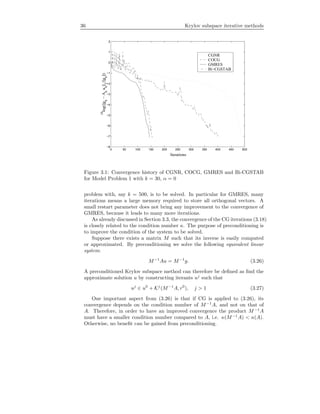
3.1 Number of iterations of several Krylov subspace methods to reach
convergence for Model Problem 1. kh = 0.625 (∼ 10 grid points
per wavelength) . . . . . . . . . . . . . . . . . . . . . . . . . . . . 35
3.2 Number of iterations of several preconditioned Krylov subspace
methods for Model Problem 1. The preconditioner is ILU(0).
kh = 0.625 (∼ 10 grid points per wavelength) . . . . . . . . . . . 39
3.3 Number of iterations of several preconditioned Krylov subspace
methods for Model Problem 1. The preconditioner is ILU(0.01).
kh = 0.625 (∼ 10 grid points per wavelength). COCG stagnates
for k ≥ 20 . . . . . . . . . . . . . . . . . . . . . . . . . . . . . . . 39
4.1 Computational performance of GMRES to reduce the relative
residual by order 7. for 2D closed-off problem. The precondi-
tioner is the shifted Laplace operator. 10 grid points per wave-
length are used (kh = 0.625). The preconditioners are inverted
by using a direct solver . . . . . . . . . . . . . . . . . . . . . . . . 54
4.2 Computational performance of preconditioned GMRES to solve
Model Problem 1. The preconditioner is the shifted Laplace pre-
conditioners: Mh,(0,0), Mh,(−1,0) and Mh,(0,1). 10 grid points per
wavelength are used (kh = 0.625) . . . . . . . . . . . . . . . . . . 55
4.3 Computational performance of GMRES (in terms of number of
iterations) to solve the “close-off” problem (see Example 4.1) with
different grid resolutions . . . . . . . . . . . . . . . . . . . . . . . 63
4.4 Computational performance (in terms of number of iterations)
of GMRES, CGNR, and Bi-CGSTAB to solve the three-layer
problem. The preconditioner is the shifted Laplace operator; 30
grid points per kref are used . . . . . . . . . . . . . . . . . . . . . 64](https://image.slidesharecdn.com/erlangga-160128071050/85/Erlangga-11-320.jpg)

![Chapter 1
Introduction
We are concerned with the numerical solution of wave problems in two and three
dimensions. The wave problems to be considered are modeled by means of the
Helmholtz equation, which represents time-harmonic wave propagation in the
frequency domain.
The Helmholtz equation finds its applications in many fields of science and
technology. For example, the Helmholtz equation has been used to investigate
acoustic phenomena in aeronautics [64] and underwater acoustics [41, 4]. The
Helmholtz equation is also solved in electromagnetic applications, e.g. in pho-
tolithography [96]. Due to recently increased interest in a more efficient solver
for migration in 3D geophysical applications the use of the Helmholtz equation
is also investigated in that field [75, 80].
In this thesis we will focus on the application of the Helmholtz equation in
geophysics. The method which is proposed and explained in this thesis can,
however, be used for any class of problems related to the Helmholtz equation.
1.1 Motivation: seismic applications
In geophysical applications, seismic information on the earth’s subsurface struc-
tures is very important. In the petroleum industry, e.g., accurate seismic in-
formation for such a structure can help in determining possible oil reservoirs
in subsurface layers. This information, or in particular an image of the earth’s
subsurface, is gathered by measuring the times required for a seismic wave to re-
turn to the surface after reflection from the interfaces of layers of different local
physical properties. The seismic wave is usually generated by shots of known
frequencies, placed on the earth’s surface, and the returning wave is recorded
by instruments located along the earth’s surface. Variations in the reflection
times from place to place on the surface usually indicate structural features of
the strata up to 6,000 m below the earth’s surface. One technique, which is
popular nowadays, to postprocess the seismic data and construct the image of
the earth’s subsurface is migration.](https://image.slidesharecdn.com/erlangga-160128071050/85/Erlangga-15-320.jpg)
![2 Introduction
Migration is a technique to focus the seismic waves such that the exact
information of the reflector/secondary sources on the subsurface is correctly
known. A modern migration technique is based on the wave equation, originally
proposed by Claerbout in the early 1970s, which is based on the finite-difference
approach [16].
To keep the computational cost acceptable, the wave equation is usually
replaced by a one-way or paraxial approximation [10, 17, 25, 28, 60]. This
approximation is in most cases valid for not too large velocity contrasts and not
too wide angles of incidence. With the continuing increase in computer power,
it may be worthwhile to develop finite-difference two-way or full wave-equation
migration techniques, without making the approximations needed for ray-based
or one-way migration methods [107].
Nowadays, for the imaging of seismic data, the industry is gradually moving
from 1D models based on ray-based techniques to 2D/3D finite-difference wave-
equation migration. Ray-based methods are difficult to use or may even fail in
complex earth models and in the presence of large velocity contrasts. Wave-
equation migration can better handle these situations.
In two-dimensional space, two-way wave-equation migration can be carried
out efficiently by working in the frequency domain. In that case, the linear
system arising from the discretization of the two-way wave equation is solved
once with a direct solution method for each frequency. The result can be used
for the computation of all the wave fields for all shots and also for the back-
propagated receiver wave fields. The latter correspond to the reverse-time wave
fields in the time domain [72, 75, 80]. This makes the 2D method an order of
magnitude faster than its time-domain counterpart when many shots need to
be processed.
Time-domain reverse-time migration requires the storage of the forward and
time-reversed wave fields at time intervals to avoid aliasing. These wave fields
are correlated to obtain a partial migration image for each shot. Adding over all
shots provides the desired result. In the frequency domain, only one forward and
one back-propagated wave field need to be stored. They are simply multiplied
to obtain a partial migration image. The summation over shots and frequencies
produces the final migration image. In this way, a substantial reduction of
storage requirement is obtained.
Because direct solvers are computationally out of reach in 3D, a suitable iter-
ative method for the two-way wave equation is needed. This iterative method,
however, must be applied for each shot and each back-propagated wave field
computation. Differently, a direct method is employed only once to compute an
LU-decomposition of the linear system. Once this costly step has been carried
out, the computation of wave fields for all shots and receiver wave fields can be
carried at a small computational cost [72]. This attractive feature, that makes
the frequency-domain approach so efficient in 2D is lost when we use an iterative
method.
If we ignore storage requirements and only consider computational time, a
frequency-domain formulation can only compete with the time-domain approach
if the work involved in the iterations times the number of frequencies is signifi-](https://image.slidesharecdn.com/erlangga-160128071050/85/Erlangga-16-320.jpg)
![1.2 The Helmholtz equation 3
cantly less than the work needed for doing all the time steps in the time-domain
method [36]. We will return to this issue in Section 1.5.
From its formulation, the time-harmonic Helmholtz equation looks easy and
straightforward to solve as it can be considered as the Poisson equation with ze-
roth order perturbation. Many efficient numerical methods have been developed
for the Poisson equation. This extra term, however, appears in the Helmholtz
equation with the wrong sign. Therefore, the Helmholtz equation does not in-
herit the same nice properties the Poisson equation has. This perturbation is
actually the source of complications when one tries to numerically solve the
Helmholtz equation.
In the last three decades attempts to iteratively solve the Helmholtz equation
have been made by many authors. The paper of Bayliss, Goldstein and Turkel
[12], that appeared in the early 1980s, can be considered as the first publication
which shows efficient implementation of an iterative method (i.e. conjugate gra-
dients) on the Helmholtz equation. The follow-up paper by Gozani, Nochshon
and Turkel [51] includes multigrid as a preconditioner in the conjugate gradient
algorithm. Because the methods are not of highest efficiency for high wavenum-
ber (or frequency) problems, many contributions have been made since. Work
in [12] and [51], however, gives cause for optimism that a well-designed iterative
method can be used to solve the Helmholtz equation with a greater efficiency
than a traditional direct solver, especially in three-dimensional space.
Ideally, the performance of an iterative method for the Helmholtz equation
should be independent of both the grid size and the wavenumber. As inde-
pendence of the grid size can sometimes be easily achieved, the dependence
on the wavenumber is the difficult part to tackle. Iterative methods typically
suffer from efficiency degradation when the wavenumber is increased. The re-
search in this thesis is geared towards an iterative method whose performance
is independent of grid size and (only mildly) of the wavenumber.
1.2 The Helmholtz equation
In this section we derive the Helmholtz equation, which is used in the frequency-
domain wave equation migration. The discussion is given for fluids and solids,
the media which are present in the earth subsurface. For fluids, the Helmholtz
equation can be obtained from the Euler equations, after applying a lineariza-
tion; see [29, 49]. We, however, show a different approach to derive the Helmholtz
equation, as used in [16]. This approach is unified approach, that can be applied
to fluids and solids. Furthermore, the relationship between the wave equation
for fluids and solids is clearly seen.
The basic equations used for the derivation of the wave equation are the
equation of motion (governed by Newton’s second law) and the Hooke law,
which relates particle velocity in space and pressure in time. We first discuss
the wave equation for fluids.
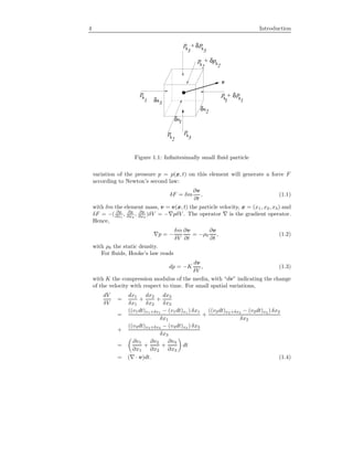
Consider an infinitesimally small fluid element with a volume δV in a domain
Ω = R3
, as depicted in Figure 1.1. By assuming zero viscosity, the spatial](https://image.slidesharecdn.com/erlangga-160128071050/85/Erlangga-17-320.jpg)
![8 Introduction
with 0 ≤ α 1 indicating the fraction of damping in the medium. In geophysical
applications, that are of our main interest, this damping can be set up to 5%;
(α = 0.05).
The “damped” Helmholtz equation expressed by (1.26) is more general than
(1.23) and (1.25). Therefore, due to its generality we prefer to use the Helmholtz
equation (1.26) throughout the presentation. Whenever necessary, the “stan-
dard” Helmholtz equation can be recovered from (1.26) by setting α = 0.
Remark 1.2.4 Scaling. Assume that the physical domain has a characteristic
length l and consider a nondimensional domain [0, 1]3
. The nondimensional
length is determined as x1 = x1/l, x2 = x2/l and x3 = x3/l. Thus,
∂
∂x1
=
1
l
∂
∂x1
,
∂2
∂x2
1
=
1
l
2
∂2
∂x2
1
, and so on.
Substituting these relations into (1.26) results in
−∆u(x) − (1 − αˆj)k
2
(x)u(x) = g(x), x = (x1, x2, x2), in Ω = (0, 1)3
,
with the wavenumber in the non-dimensional domain, denoted by k, can be re-
lated to the physical quantities in the physical domain by the relation
k = 2πfl/c. (1.27)
In the discussion to follow we will use the notation k for wavenumbers regardless
of the domain we are considering. However, the meaning should be clear from the
context. If we consider a unit domain, the wavenumber should be dimensionless.
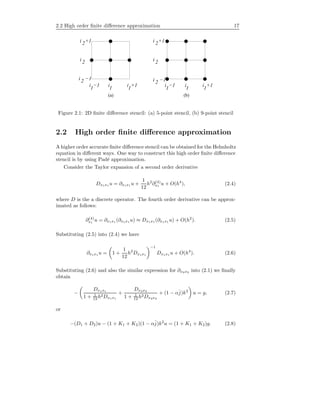
1.3 Boundary conditions
For a partial differential equation, of the form (1.23), (1.25) or (1.26), proper
boundary conditions are required. These boundary conditions should be chosen
such that the resulting problem is well-posed. In general, one can identify two
types of boundary conditions. The first type is a boundary condition for waves
propagating to infinite distance. The second type is related to waves scattered
by obstacles in a medium.
A boundary condition at infinity can be derived by considering the phys-
ical situation at infinity [49]. This situation can be viewed directly from the
Helmholtz equation (1.23) if we consider a domain Ω with a homogeneous
medium. Assume spherical symmetric waves propagating from a source or a
scatterer in the domain Ω. In most cases, close to the source/scatterer this
assumption is easily violated; there the waves are arbitrary and more complex
than just spherical. We assume, however, that at infinity these complex waves
are disentangled and become spherical. Under this assumption, the problem](https://image.slidesharecdn.com/erlangga-160128071050/85/Erlangga-22-320.jpg)
![10 Introduction
The radiation condition (1.30) is only satisfied at infinity. In a numerical
model, this condition is approximately satisfied, as an infinite domain is always
truncated to a finite region. Therefore, a numerical radiation condition is re-
quired for boundaries at finite distance, which mimics the radiation condition
at infinity. This will be addressed in Chapter 2.
In the scattering situation, additional boundary conditions inside Ω repre-
senting the presence of the obstacles should be added. Consider an impenetrable
obstacle D in Ω with boundary Γs = ∂D. We distinguish two types of bound-
ary conditions commonly used for scattering problems. In the case of sound-soft
obstacles, the velocity of the total wave (i.e. the sum of the incoming wave φi
and the scattered wave φs
) vanishes at Γs, i.e. φ = 0 on Γs. This is known
as the Dirichlet boundary condition. For the case of sound-hard obstacles, the
condition on Γs leads to a Neumann condition: ∂φ/∂n = 0, implying a condition
of a vanishing normal velocity on the scatterer surface.
1.4 Direct methods and iterative methods
Numerical approximations based on finite differences/volumes/elements require
the solution of a sparse, large linear system of equations. There are in general
two classes of methods to solve a linear system: direct methods and iterative
methods.
Direct methods are basically derived from Gaussian elimination. They are
well-known for their robustness for general problems. However, Gaussian elimi-
nation is not favorable for sparse linear systems. During the elimination process,
zero elements in the matrix may be filled by non-zero entries. This is called fill-
in and gives rise to two complications: (i) extra computer storage required to
store the additional non-zero entries, (ii) extra computational work during the
elimination process.
In many problems, a reordering strategy or pre-processing (e.g. nested dis-
section) technique can be used to modify the structure of the matrix such that
Gaussian elimination can be performed more efficiently (see e.g. [48]). Never-
theless, it is also possible that the pre-processing adds some more computational
work.
Iterative methods, on the other hand, rely primarily on matrix-vector multi-
plications. An example of a simple iterative method is the Jacobi iteration. In
the Jacobi iteration, the solution of linear system is iteratively obtained from a
recursion consisting of one matrix-vector multiplication, starting with a given
initial solution. A matrix-vector multiplication is a cheap process, requiring only
O(N) arithmetic operations per iteration with N the number of unknowns. If
the method converges after a finite small number of iterations, the method would
be efficient.
Iterative methods, however, are not always guaranteed to have fast conver-
gence. In fact there are many situations for iterative methods to diverge. In
such cases, iterative methods do not offer any advantage as compared to direct
methods.](https://image.slidesharecdn.com/erlangga-160128071050/85/Erlangga-24-320.jpg)
![1.5 Time-domain vs. frequency-domain solver 11
Table 1.1 compares the typical complexities of different solvers for a banded
linear system obtained from a finite difference discretization of the 2D Poisson
equation. The size of the linear system to solve is N ×N, where N is the number
of unknowns. The iterative methods converge to a tolerance . Conjugate
gradients and multigrid, two advanced iterative methods, are later discussed in
this thesis.
Table 1.1: Some two-dimensional Poisson solvers with arithmetic complexity
[92]. N is the number of unknowns
Method Complexity
Gauss elimination O(N2
)
Jacobi/Gauss-Seidel iteration O(N2
log )
Successive over relaxation (SOR) O(N3/2
log )
Conjugate gradient O(N3/2
log )
Nested dissection [48] O(N3/2
)
Alternating-direction iteration (ADI) [101] O(N log N log )
Multigrid (iterative) O(N log )
Multigrid (FMG) O(N)
For a sparse, large linear system, direct methods become impractical. This is
typical for problems in three-dimensional space. The complexity of the method
becomes O(N3
) and storage requirement can be up to O(N2
) due to fill-in.
Therefore, for three-dimensional problems iterative methods are the method of
choice. In the case of slow convergence or even divergence remedies based on
theory often exist.
The Helmholtz equation is one of the problems for which iterative methods
typically result in an extremely slow convergence. For reasons explained system-
atically in Chapters 2 and 3, the Helmholtz equation is inherently unfavorable
for iterative methods. However, with a proper remedy, e.g. with a good pre-
conditioner (to be discussed in Chapters 4 and 5), an efficient iterative method
can be designed.
Conjugate gradients and conjugate-gradient-like methods have been used in
[12], [51], [47] and [64] to solve the Helmholtz equation. ADI is used in [32].
Multigrid implementations are found in [22], [100], [65], [33] and [63].
1.5 Time-domain vs. frequency-domain solver
As mentioned in Section 1.1, to make a frequency-domain solver competitive
with the time-domain approach for geophysical applications, we require that
the work for the iterations times the number of frequencies is significantly less
than the work needed for doing all the time steps in the time-domain method.
In this section we elaborate on this subject, based on a complexity analysis [36].](https://image.slidesharecdn.com/erlangga-160128071050/85/Erlangga-25-320.jpg)
![12 Introduction
The basis for the performance prediction is the well-known time-domain
approach complexity. With ns the number of shots and nt the number of time
steps, the time-domain complexity is ns nt O(N), with N again the number
of unknowns. Stability requirements usually dictate nt = O(N1/d
), with d =
1, . . . , 3 the dimension. So, the overall complexity of the time-domain method
is ns O(N1+1/d
) for ns shots.
Suppose that there exists in frequency domain an efficient iterative method
for the Helmholtz equation with a complexity of order O(N) per iteration step.
With nf the number of frequencies, the overall complexity of the iterative solver
is ns nf nit O(N), with nit the number of iteration. The choice of the grid spac-
ing is determined by the maximum wavelength that can be accurately repre-
sented by the discretization. This implies that nf = O(N1/d
) if the maximum
frequency in the data is adapted to the grid spacing, whereas nf is indepen-
dent of N as soon as the grid is finer than required to accurately represent the
highest frequency in the data. In practice, one generally operates in the first
regime where nf = O(N1/d
). With these considerations, the complexity of the
iterative frequency-domain solver is ns nit O(N1+1/d
). From this estimate, the
optimal iterative frequency-domain solver would have the same complexity as
the time-domain solver if nit = O(1).
For a comparison between two solvers, however, the actual multiplicative
constants in the cost estimates also play an important role. The complexity of
the time-domain solver is Ct ns N1+1/d
and of the iterative frequency-domain
solver Cf ns nit N1+1/d
, with constants Ct and Cf . If one constant is several
orders of magnitude smaller than the other, a cost comparison of the meth-
ods cannot be based on considerations that involve O(n), O(nf ), etc., only.
This is observed in 2D migration problems presented in [74], where nested
dissection is used in the frequency domain. From complexity analysis, the
time-domain approach shows a better asymptotic behavior than the frequency
domain approach. Actual computations reveal, however, that the frequency-
domain method is about one order of magnitude faster than the time-domain
approach. The multiplicative constant for the frequency-domain direct solver
is apparently far smaller than the one for the time-domain solver. The reason
is that the number of frequencies needed is smaller than the number of time
steps imposed by the stability condition of the time-domain solver [75]. This
result gives an indication that if an iterative method with complexity of O(N)
can be made convergent after an O(1) number of iterations, the method can be
competitive. As in 3D direct methods become out of question, the importance
of an efficient iterative method becomes more obvious.
1.6 Scope of the thesis
This thesis deals with numerical methods for solving the Helmholtz equation in
two and three dimensions, with the following characteristics:
(i) the property of the medium (in terms of the local speed of sound, c) can
vary; i.e, heterogeneity is present in the medium,](https://image.slidesharecdn.com/erlangga-160128071050/85/Erlangga-26-320.jpg)
![1.7 Outline of the thesis 13
(ii) the wavenumber k can be very large, e.g. ∼ 1000 in a unit square domain.
We focus on iterative methods within the classes of Krylov subspace and
multigrid methods. As already mentioned, we aim at a method whose perfor-
mance is independent of grid size and wavenumber. By using a proper precon-
ditioner, the performance of the method can be made grid-independent. The
method presented in this thesis shows linear dependence on the wavenumber,
with only small constant.
Furthermore, we focus on linear systems obtained from finite difference dis-
cretizations. This is, however, not a limitation of the iterative method discussed
here. The method can handle different types of discretizations without losing
its efficiency and robustness.
Numerical results presented in this thesis are based on problems arising from
geophysical applications with extremely high wavenumbers. But, the method
developed in this thesis can also be used in other applications governed by the
Helmholtz equation.
1.7 Outline of the thesis
The outline of the thesis is as follows.
• In Chapter 2, discretization methods for the Helmholtz equation are dis-
cussed. The discussion emphasizes finite differences suitable for geophys-
ical applications.
• In Chapter 3 iterative methods are introduced for solving the resulting
linear systems. These include the basic iterative (Jacobi and Gauss-Seidel)
and Krylov subspace methods, which are the important and principal
methods in our solver. Some preconditioners which are relevant for Krylov
subspace methods are also discussed.
• Chapter 4 is devoted to a novel class of preconditioners for the Helmholtz
equation, called complex shifted Laplace preconditioners, which is an im-
portant ingredient in the method presented in this thesis and introduced
by us in a series of papers [37, 38, 40]. Discussions include the spectral
properties which are helpful to evaluate the convergence of the Krylov
subspace methods.
• In Chapter 5 the multigrid method is introduced. In particular, we discuss
the use of multigrid to approximately invert the complex shifted-Laplace
operator.
• In Chapter 6 a multigrid-based preconditioner especially designed for the
Helmholtz equation is introduced and discussed. Numerical tests for two-
dimensional problems are presented.
• Chapter 7 discusses the extension of the method to three dimensions and
shows results for three-dimensional problems.](https://image.slidesharecdn.com/erlangga-160128071050/85/Erlangga-27-320.jpg)
![14 Introduction
• In Chapter 8 we draw some conclusions and give remarks and suggestions
for future work.
1.8 About numerical implementations
In this thesis computations are performed for a variety of model problems. In
the early stages of the research a not-the-fastest computer was used to produce
the convergence results. As a new, faster computer has replaced the old one, the
numerical results are updated to have more impressing CPU times. Therefore,
one finds that some results here differ with the results that appeared in early
publications, e.g. in [38].
To reproduce the numerical results presented in this thesis, we have used
a LINUX machine with one Intel Pentium 4, 2.40 GHz CPU. This machine is
equipped with 2 GByte of RAM and 512 KByte of cache memory. For small
problems, MATLAB has been used for coding. GNU’s Fortran 77 compiler is
used mainly for large problems.](https://image.slidesharecdn.com/erlangga-160128071050/85/Erlangga-28-320.jpg)
![Chapter 2
Finite differences for the
Helmholtz equation
The standard procedure for obtaining a numerical solution of any partial differ-
ential equation (PDE) is first replacing the equation by its discrete formulation.
For the Helmholtz equation, there are many methods to realize this, including
the boundary element method (BEM) and the finite element method (FEM).
BEM, which typically results in a small but full linear system after discretiza-
tion, will not be discussed here. References [57], [58], [59], [7], [8], [9] and
[31], amongst others, discuss FEM for the Helmholtz equation. We focus on
finite difference methods (FDM). All numerical results presented in this thesis
are obtained from a finite difference approximation of the Helmholtz equation.
Furthermore, structured equidistant grids are employed.
A general discussion on finite difference methods for partial differential equa-
tions can be found, e.g. in [88]. The development of a high order FDM is given,
e.g. in [68], [13], [66] and [90]. There exist different finite difference approx-
imations for the Helmholtz equation (see e.g. [54], [85] and [61]). Here we
consider two of them: the pointwise representation and a high order representa-
tion. The pointwise representation is usually related to the so-called five-point
stencil. Dispersion and anisotropy properties of the two representations are
briefly discussed in Section 2.3.
In geophysical applications finite differences are widely used. One practical
reason is that the domains used in these applications are often simple (e.g. rect-
angular or box shape) and can be well fitted by regular finite difference meshes.
For Helmholtz problems with a complex geometry arising from scattering prob-
lems, finite elements are often the method of choice.
For ease of presentation, we consider the “damped” Helmholtz equation
(1.26) in Ω ⊂ R2
. Extension to three-dimensional space is straightforward.](https://image.slidesharecdn.com/erlangga-160128071050/85/Erlangga-29-320.jpg)
![18 Finite differences for the Helmholtz equation
where
D1 = Dx1x1 + Dx2x2 (2.9)
D2 =
h2
6
Dx1x1 Dx2x2 (2.10)
K1 =
h2
12
(Dx1x1 + Dx2x2 ) (2.11)
K2 =
h4
144
Dx1x1 Dx2x2 (2.12)
Equation (2.8) is called the point-wise Pad´e approximation of the Helmholtz
equation. Harari and Turkel [54] (and also Singer and Turkel in [85]) propose
a generalization to this approximation by introducing a free parameter γ ∈ R.
This parameter is tuned such that the dispersion or the anisotropy is minimal.
The following 9-point stencil is due to Harari and Turkel [54], for α = 0:
Ah,9p
∧
= −
1
h2
1
6 + γ (kh)2
144
2
3 + (6−γ)(kh)2
72
1
6 + γ (kh)2
144
2
3 + (6−γ)(kh)2
72 −10
3 + (24+γ)(kh)2
36
2
3 + (6−γ)(kh)2
72
1
6 + γ (kh)2
144
2
3 + (6−γ)(kh)2
72
1
6 + γ (kh)2
144
. (2.13)
It can be shown that this scheme is consistent for kh → 0 and O(h4
) accurate for
constant wavenumber and uniform grids. The scheme, however, is only O(h3
)
for nonconstant wavenumber and non-uniform grids.
Remark 2.2.1 The Pad´e approximation for the 3D Helmholtz equation is given
in Appendix A.
Remark 2.2.2 A non standard 9-point finite difference approximation is also
proposed by [61]. The approach is based on a splitting of the Laplacian term
into two parts: one in grid line direction and one in cell-diagonal direction,
with some weights. It can be shown that the dispersion and anisotropy can also
be minimized in this case.
2.3 Dispersion and anisotropy
In order to illustrate the dispersion and anisotropy properties of a discretization
scheme, we define two parameters which characterize wave propagations [54]:
cp =
ωw
k
, cg =
∂ωw
∂k
, (2.14)
which are called the phase velocity and the group velocity, respectively. For
homogeneous and isotropic continuous media, cp = cg = c0; i.e. the media is
non-dispersive.
In a discrete formulation the non-dispersive property no longer holds. In-
stead, we have that
ch
p =
ωw
kh
=
k
kh
c0, ch
g =
∂ωw
∂kh
=
∂kh
∂k
−1
c0, (2.15)](https://image.slidesharecdn.com/erlangga-160128071050/85/Erlangga-32-320.jpg)
![2.3 Dispersion and anisotropy 19
where kh
= f(kh), depending on the discretization. For the 5-point stencil, we
have that [54]:
ch
p
c0
=
kh
arccos(1 − (kh)2/2)
, (2.16)
ch
g
c0
= 1 − (kh)2/4. (2.17)
Thus, for the 5-point stencil the phase and group velocity are slower than the
speed of sound c0.
For the 9-point stencil (2.13), the phase and group velocity along the grid
lines are determined respectively as:
ch
p
c0
=
kh
arccos((1 − 5(kh)2/12)/(1 + (kh)2/12))
, (2.18)
ch
g
c0
= 1 − (kh)2/6 (1 + (kh)2
/12). (2.19)
Along the grid line, for a resolution up to a minimum of 4 grid points per
wavelength (i.e. kh < 1.57), the 9-point stencil is less dispersive compared to the
5-point stencil. In fact, the error of the 9-point stencil falls within 7 % compared
to non-dispersion solution. The 5-point stencil, however, is still accurate if more
than 10 grid points per wavelength are used (or, equivalently, if kh < 0.625).
Similarly, one can derive the phase and group velocity of discrete cases for
plane waves oriented at an angle θ with respect to the grid lines. An extreme
case occurs when the wave is in the direction of the cell’s diagonal (θ = π/4).
For the 5-point stencil we then have
ch
p
c0
=
kh
√
2 arccos(1 − (kh)2/4)
, (2.20)
ch
g
c0
= 1 − (kh)2/8, (2.21)
and for the 9-point stencil, the phase and group velocities can be determined
from the relation
kh
h =
√
2 arccos
6 1 + (1 − γ)(kh)4/144 − (4 + (6 − γ)(kh)2
/12)
2 + γ(kh)2/12
. (2.22)
In both cases, the phase and group velocity are slower than the speed of
sound c0. For the 5-point stencil, however, the scheme is less dispersive for waves
oriented in the direction of cell diagonals compared to waves in the direction
of grid lines. The value γ = 2/5 results in a 9-point discretization stencil with
minimal dispersion in the direction of cell diagonals. If γ = 14/5 the difference
between dispersion in the direction of cell diagonals and grid lines is minimal.
Thus, γ = 14/5 leads to a 9-point stencil with minimal anisotropy. We refer the
reader to [54] for a more detailed discussion on this subject.](https://image.slidesharecdn.com/erlangga-160128071050/85/Erlangga-33-320.jpg)
![20 Finite differences for the Helmholtz equation
Remark 2.3.1 For the second order scheme, however, the quantity kh is not
sufficient to determine the accuracy of the numerical solution of the Helmholtz
equation [13]. The quantity k3
h2
is also found important in determining the
accuracy in the L2
norm, especially at high wavenumbers.
Remark 2.3.2 In our numerical tests we often use the five-point finite differ-
ence stencil on the minimum allowable grid resolution kh = 0.625. Table 2.1
displays the number of grid points for kh = 0.625.
Table 2.1: Number of grid points employed, related to the wavenumber, so that
kh = 0.625.
k: 10 20 30 40 50 80 100 150 200 500 600
N(= 1/h): 8 16 32 64 80 128 160 240 320 800 960
2.4 Numerical boundary conditions
In Chapter 1 we have formulated a condition for the radiation boundary. This
condition, however, is only satisfied in an infinite domain. For computational
purposes extending the domain to infinity is not practical due to, e.g., restricted
hardware resources. Therefore, we often truncate the domain in such away
that a physically and computationally acceptable compromise is reached. In
this truncated domain, the non-reflecting boundary condition given in (1.30) is,
however, no longer valid.
In [70] and [67] non-local boundary conditions are proposed to mimic the
radiation condition at infinity. Despite their accuracy for any direction of wave
incidence, the inclusion of this type of boundary condition in the discretization
is not practical because of the non-locality. Enquist et al in [34] proposed local
boundary conditions for a truncated domain; see also [26], [27]. Different types
of local boundary conditions have also been proposed elsewhere; see, e.g., in [56],
[50] and the references therein. In this thesis, we limit ourselves to the local
boundary conditions proposed in [34], either in the first order or the second
order formulation.
In our case we consider a rectangular domain which is typically used in
geophysics. We distinguish on a boundary Γ: faces, edges and corners. For each
part of Γ we have the following boundary conditions (see [26, 34, 55, 11]):
Faces:
B2u|face := ±
∂u
∂xi
− ˆjku −
ˆj
2k
3
j=1,j=i
∂2
u
∂x2
j
= 0, i = 1, . . . , 3. (2.23)
Here xi is the coordinate perpendicular to the face.](https://image.slidesharecdn.com/erlangga-160128071050/85/Erlangga-34-320.jpg)
![2.5 The properties of the linear system 21
Edges:
B2u|edge := −
3
2
k2
u − ˆjk
3
j=1,j=i
±
∂u
∂xj
−
1
2
∂2
u
∂x2
i
= 0, i = 1, . . . , 3, (2.24)
with xi the coordinate parallel to the edge.
Corners:
B2u|corner := −2ˆjku +
3
i=1
±
∂u
∂xi
= 0. (2.25)
In (2.23)–(2.25) the ± sign is determined such that for out going waves the
non-reflecting condition is satisfied.
For the second order derivatives, to retain the same order of accuracy as in
the interior the same discretization is used as for the Helmholtz operator.
In Chapters 4 and 5 we implement the first order boundary condition on the
faces described by [34]
B1u|face :=
∂
∂η
− ˆjk u = 0, (2.26)
with η the outward normal component to the boundary. This boundary con-
dition (2.26) is straightforward to discretize (either with one-sided or central
schemes), but it is not accurate for inclined outgoing waves. In Chapter 6
boundary conditions of the form (2.23)–(2.25) are implemented.
Remark 2.4.1 In practice the use of the second order radiation conditions
sometimes is not sufficient to reduce reflections. In the last decade a new and ac-
curate boundary condition for wave equations, called the perfectly matched layer
(PML) has attracted many researchers. PML is first introduced in Berenger’s
two papers [14] and [15]. Contributions to the well-posedness of PML are given
by Abarbanel et al in [1] (and also [2]). Applications of PML in wave problems
can be found, e.g. in [95] and [93]. In our research, the use of PML is not
investigated in detail.
Instead, we will use in some of numerical tests (in Chapter 6) a classical
method similar to PML, which is dubbed as “sponge” layers (or absorption lay-
ers). These layers are added around the physical domain whose functions is
to damp the out going waves. Therefore, the “damped” Helmholtz equation is
used in this layer. On the boundaries of the absorption layers, the first order
Sommerfeld radiation condition is imposed.
2.5 The properties of the linear system
Discretization of the Helmholtz equation (2.1) and boundary conditions (2.23)–
(2.25) (or (2.26)) leads to a linear system
Ahuh = gh, Ah ∈ CN×N
, uh, gh ∈ CN
. (2.27)](https://image.slidesharecdn.com/erlangga-160128071050/85/Erlangga-35-320.jpg)
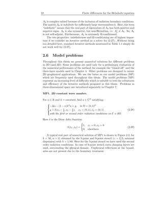
![2.6 Model problems 23
x−axis
y−axis
0 0.2 0.4 0.6 0.8 1
0
0.2
0.4
0.6
0.8
1
x−axis
y−axis
0 0.2 0.4 0.6 0.8 1
0
0.2
0.4
0.6
0.8
1
Figure 2.2: Numerical solution (real part) at k = 50, α = 0 for the model
problem MP1 with k constant. Left: 5-point stencil with 2nd order radiation
boundary conditions. Right: 9-point stencil (γ = 2/5) and 1st order radiation
boundary conditions imposed on the damping layer
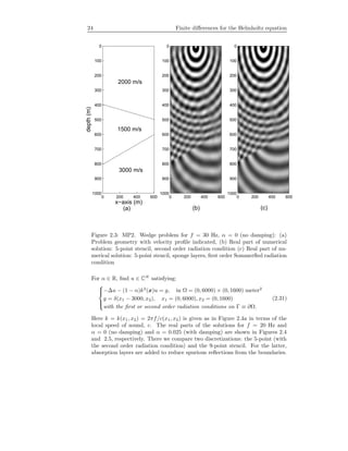
MP2. 2D wedge problem.
This is a problem which mimics three layers with a simple heterogeneity, taken
from [81].
For α ∈ R, find u ∈ CN
satisfying:
−∆u − (1 − α)k2
(x)u = g, in Ω = (0, 600) × (0, 1000) meter2
g = δ(x1 − 300, x2), x1 = (0, 600), x2 = (0, 1000)
with the first or second order radiation conditions on Γ ≡ ∂Ω.
(2.30)
So, k = k(x1, x2) = 2πf/c(x1, x2) is given as in Figure 2.3a in terms of the local
speed of sound, c. The real parts of the solutions for f = 30, h = 2.6 m and with
α = 0 are shown in Figure 2.3b and 2.3c. In Figure 2.3b the 5-point stencil
is used with the second order radiation conditions. In Figure 2.3c the 5-point
stencil is used with sponge layers added. At the boundaries of the sponge layers,
the first order Sommerfeld radiation condition is imposed.
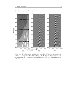
MP3. 2D Marmousi problem.
This problem mimics the earth’s subsurface layer with a complex heterogeneity
[18, 81]. It represents a part of the full Marmousi problem, a relevant and diffi-
cult test in geophysics.](https://image.slidesharecdn.com/erlangga-160128071050/85/Erlangga-37-320.jpg)
![28 Krylov subspace iterative methods
Thus,
uj
= F−1
g + (I − F−1
A)uj−1
= uj−1
+ F−1
rj−1
, (3.4)
with rj−1
:= g − Auj−1
the residual after the (j − 1)-th iteration, and I the
identity matrix. Equation (3.4) is called the basic iterative method.
The basic iteration is distinguished by the way the splitting is chosen. If
the splitting is defined by A = D − E, where D = diag(A), the Jacobi iteration
results, namely
uj
= uj−1
+ D−1
rj−1
. (3.5)
The Gauss-Seidel iteration is obtained from the splitting A = L − U, where L
and U are lower and upper triangular matrices, respectively. This iteration is
written as
uj
= uj−1
+ L−1
rj−1
. (3.6)
3.2 Krylov subspace methods
The Krylov subspace iteration methods are developed based on a construction
of consecutive iterants in a Krylov subspace, i.e. a subspace of the form
Kj
(A, r0
) = span r0
, Ar0
, A2
r0
, . . . , Aj−1
r0
, (3.7)
where r0
:= g − Au0
is the initial residual, with u0
the initial solution. The
dimension of Kj
is equal to j and increases by one at each step of the approxi-
mation process.
The idea of Krylov subspace methods can be outlined as follows. For an
initial solution u0
, approximations uj
to the solution u are computed every step
by iterants uj
of the form
uj
∈ u0
+ Kj
(A, r0
), j > 1. (3.8)
The Krylov subspace Kj
is constructed by the basis v1
, v2
, . . . , vj
, where
V j
= [v1
, v2
, . . . , vj
] ∈ Kj
. (3.9)
With residual rj
= g − Auj
, (3.7) gives an expression for the residual at the
j-th step
rj
= r0
− AV j
yj
, (3.10)
where yj
∈ CN
and uj
= u0
+ V j
yj
. From (3.10) we observe that Krylov
subspace methods rely on constructing the basis of V j
and the vector yj
. In
general we identify two methods that can be used for constructing the basis of](https://image.slidesharecdn.com/erlangga-160128071050/85/Erlangga-42-320.jpg)
![3.3 Conjugate gradient 29
V j
: Arnoldi’s method and Lanczos’ method. The vector yj
can be constructed
by a residual projection or by a residual norm minimization method.
In the following subsections, we present some Krylov subspace algorithms,
that are used in numerical simulations in this thesis. In particular, we discuss
the Conjugate Gradient (CG) (see e.g. [83]), GMRES [84] and Bi-CGSTAB
[97] algorithms. CG can be used to derive CGNR (which can be used for the
Helmholtz equation) and as a basis for COCG [98], a CG-like method for com-
plex, symmetric matrices.
Some authors, e.g. [47] have also used QMR [46] and its symmetric version
SQMR [44] for the Helmholtz equation.
3.3 Conjugate gradient
Here we assume the matrix A to be symmetric, positive definite (SPD). In CG
one constructs a vector uj
∈ Kj
(A, r0
) such that u − uj
A is minimal, where
u A = (Au, u)
1
2 . For this purpose, the vector uj+1
is expressed as
uj+1
= uj
+ αj
pj
, (3.11)
where pj
is the search direction. The residual vectors satisfy the recurrence
rj+1
= rj
− αj
Apj
. (3.12)
For all rj
’s to be orthogonal, the necessary condition is that (rj+1
, rj
) = 0. Here
(a, b) denotes the standard Hermitian inner product a∗
b, which reduces to the
transposed inner product aT
b if a, b ∈ RN
. Thus,
(rj+1
, rj
) = 0 → (rj
− αj
Apj
, rj
) = 0, (3.13)
which gives
αj
=
(rj
, rj
)
(Apj, rj )
. (3.14)
Since the next search direction pj+1
is a linear combination of rj+1
and pj
, i.e.,
pj+1
= rj+1
+ βj
pj
, (3.15)
the denominator in (3.14) can be written as (Apj
, pj
− βj−1
pj−1
) = (Apj
, pj
),
since (Apj
, pj−1
) = 0. Also because (Apj+1
, pj
) = 0, we find that
βj
=
rj+1
, rj+1
rj , rj
. (3.16)
The CG algorithm is summarized as follows:](https://image.slidesharecdn.com/erlangga-160128071050/85/Erlangga-43-320.jpg)
![30 Krylov subspace iterative methods
Algorithm 3.1. Conjugate gradient, CG
1. Set the initial guess: u0
. Compute r0
= g − Au0
. Set p0
= r0
.
2. Do j = 0, 1, . . .
3. αj
= (rj
, rj
)/(Apj
, pj
).
4. uj+1
= uj
+ αj
pj
. If accurate then quit.
5. rj+1
= rj
− αj
Apj
.
6. βj
= (rj+1
, rj+1
)/(rj
, rj
).
7. pj+1
= rj+1
+ βj
pj
.
8. Enddo
It can be shown that this algorithm minimizes u − uj
A over Kj
(A, r0
).
Algorithm 3.1 has the nice properties that it requires only short recurrences,
one matrix/vector multiplication and a few vector updates. However, for general
matrices the algorithm may not converge, because the orthogonality condition
cannot be satisfied. In case the definiteness of A (like for the Helmholtz equa-
tion) is not guaranteed, the product (V j
)∗
AV j
=: Tj
is possibly singular or
nearly singular. Since xj
= V j
Tj
βe1, for Tj
nearly/possibly singular, xj
is
poorly determined then, see [79].
One simple remedy for the indefiniteness is to apply the CG algorithm to
the normal equations A∗
A. In this case one considers the linear system
A∗
Au = A∗
g. (3.17)
For u = 0, u∗
A∗
Au = (Ax, Ax) > 0. Hence, the product A∗
A is positive
definite. Furthermore, if A ∈ CN×N
, the product A∗
A is Hermitian, because
(A∗
A)∗
= A∗
A. Therefore, Algorithm 3.1 can be applied to the linear system
(3.17).
Direct implication of Algorithm 3.1 applied on (3.17) results in the following
algorithm, called CGNR.
Algorithm 3.2. CGNR
1. Set the initial guess: u0
. Compute r0
= g − Au0
.
2. Compute z0
= A∗
r0
. Set p0
= r0
.
3. Do j = 0, 1, . . .
4. wj
= Apj
.
5. αj
= (zj
, zj
)/(Apj
, Apj
).
6. uj+1
= uj
+ αj
pj
. If accurate then quit.
7. rj+1
= rj
− αj
Apj
.
8. zj+1
= A∗
rj+1
.
9. βj
= (zj+1
, zj+1
)/(zj
, zj
).
10. pj+1
= zj+1
+ βj
pj
.
11. Enddo
In general, Algorithm 3.2. is twice as expensive as Algorithm 3.1. Further-
more, A∗
is sometimes not readily available, meaning one has to compute A∗
each time it is required. In this situation, it is better to have an algorithm for
general matrices where A∗
needs not necessarily be computed explicitly. This](https://image.slidesharecdn.com/erlangga-160128071050/85/Erlangga-44-320.jpg)
![3.4 Conjugate orthogonal-conjugate gradient 31
is one of the two main reasons why Bi-CGSTAB (discussed in Section 3.6) is
more preferable for our problems. The other reason will be explained shortly
when we discuss the convergence of CG iterations.
For algorithms with optimality properties, like CG (and also GMRES), con-
vergence estimates can be derived. This property is essential, especially in
Chapter 4, when we are considering the convergence behavior of Krylov subspace
iterations for the Helmholtz equation. Here, we present one of the convergence
estimates of CG. We refer the reader to, e.g., [83] for more details.
Given κ = λmax/λmin, the l2 condition number of an SPD matrix A, where
λmax and λmin represent the maximum and the minimum eigenvalues of A,
respectively. The error between the exact solution uh and the approximate
solution after the j-th CG iteration can be bounded by the following upper
bound:
u − uj
A ≤ 2
√
κ − 1
√
κ + 1
j
u − u0
A. (3.18)
It is clear that CG converges faster for a matrix A with a smaller condition
number κ.
For the normal equations and A an SPD matrix, κ(A∗
A) = κ2
(A). Thus
one can immediately conclude that CGNR (Algorithm 3.2) is far less efficient
than CG. (This conclusion is generally not true for a non SPD matrix. For A
indefinite, CG may diverge, whereas CGNR will still converge, even though the
convergence is very slow.)
3.4 Conjugate orthogonal-conjugate gradient
The next short recurrence algorithm which requires only one matrix/vector mul-
tiplication can also be derived for a complex, symmetric but non-Hermitian ma-
trix A by replacing the orthogonality condition (3.13) by the so-called conjugate
orthogonality condition [98]:
(rj
, ri
) = 0 if j = i. (3.19)
Since A = AT
we have that (u, Ay) = (A
T
u, y) = (Au, y) = (y, Au). One can
prove that the vectors {r0
, . . . , rj
) form a basis for Kj+1
(A, r0
). Furthermore,
the vectors rj
are conjugate orthogonal.
Based on rj
, the solution uj+1
can be constructed in Kj+1
(A, r0
) that satis-
fies the condition that the residual rj+1
= g − Auj+1
is conjugate orthogonal to
Kj+1
(A, r0
). This results in an algorithm which is similar to CG, but with the
(Hermitian) inner product being replaced by the standard inner product. The
algorithm, called conjugate orthogonal-conjugate gradient (COCG) is coded as
follows:
Algorithm 3.3. Conjugate orthogonal-conjugate gradient (COCG)
1. Set the initial guess: u0
. Compute r0
= g − Au0
. Set p0
= r0
.
2. Do j = 0, 1, . . .](https://image.slidesharecdn.com/erlangga-160128071050/85/Erlangga-45-320.jpg)
![32 Krylov subspace iterative methods
3. αj
= (rj
, rj
)/(Apj, pj
).
4. uj+1
= uj
+ αj
pj
. If accurate then quit.
5. rj+1
= rj
− αj
Apj
.
6. βj
= (rj+1
, rj+1
)/(rj
, rj
).
7. pj+1
= rj+1
+ βj
pj
.
8. Enddo
Algorithm 3.3, however, has several drawbacks. First of all, the algorithm
is no longer optimal. This is because the error u − uj
A at every step is
not minimal. The error, therefore, is not monotonically decreasing. In many
cases, the lack of optimality condition for COCG is characterized by an erratic
convergence behavior. Residual smoothing [110] can be used to obtain a rather
monotonic decreasing convergence.
Secondly, the COCG algorithm may suffer from two kinds of breakdown. The
first breakdown is related to the quasi null-space formed in the algorithm. The
quasi null-space is characterized by the situation that for rj
= 0, (rj
, rj
) = 0.
This breakdown can be overcome by restarting the process or by switching to
another algorithm. The second breakdown is due to the rank deficiency of the
linear system for computing the coefficients yj
. This type of breakdown is,
however, uncured.
Thirdly, the condition A = AT
is often too restrictive for preconditioning.
We postpone the discussion of this issue until Section 3.8, where we introduce
preconditioners to enhance the convergence of Krylov subspace methods.
3.5 Generalized Minimal Residual, GMRES
The GMRES method is an iterative method for nonsymmetric matrices, which
minimizes the residual norm over the Krylov subspace. The GMRES algorithm
is given as follows (see Saad [83] and Saad and Schultz [84]).
Algorithm 3.4. Generalized Minimum Residual, GMRES
1. Choose u0
. Compute r0
= g − Au0
, β := r0
2 and v1
:= r0
/β
2. For j = 1, 2, . . ., m do:
3. Compute wj
:= Avj
4. For i = 1, 2, . . ., m do:
5. hi,j := (wj
, vi
), wj
:= wj
− hi,jvi
6. Enddo
7. hj+1,j = wj
2.
8. vj+1
= wj
/hj+1,j
9. Enddo
10. Compute ym
: the minimizer of βe1 − ¯Hmy 2 and um
= u0
+ V m
ym
Line 2 to 9 represent the Arnoldi algorithm for orthogonalization. In line
10, we define a minimalization process by solving a least squares problem
J(y) = g − Au 2, (3.20)](https://image.slidesharecdn.com/erlangga-160128071050/85/Erlangga-46-320.jpg)
![3.6 Bi-CGSTAB 33
where
u = u0
+ V k
y (3.21)
is any vector in Kk
. Except for line 10, the GMRES algorithm is almost identical
with the Full Orthogonalization Method (FOM) [82]. (In FOM, we compute
ym
= H−1
m (βe1), where e1 is the first unit vector.) Inserting the expression of u
(3.21) to (3.20) and making use of the following property:
AV j
= V j+1 ¯Hj (3.22)
(see Preposition 6.5 in [83]), we arrive at the following result:
J(y) = βe1 − ¯Hmy 2, (3.23)
which is subjected to minimization. In (3.23), β = r0
, and e1 ≡ {1, 0, · · · , 0}T
.
The GMRES algorithm may break down if at iteration step j, hj+1,j = 0 (see
line 8). However, this situation implies that residual vector is zero and therefore,
the algorithm gives the exact solution at this step. Hence, examination of value
hj+1,j in algorithm step 7 becomes important. For the convergence of GMRES,
the following theorem is useful.
Theorem 3.5.1 Convergence of GMRES [84]. Suppose that A is diago-
nalizable so that A = XΛX, where Λ = diag{λ1, . . . , λN } with positive real
parts. Assume that all eigenvalues are enclosed by a circle centered at Cc > 0
and having radius Rc < Cc (so the circle does not enclose the origin). Then the
residual norm at the j-th GMRES iteration satisfies the inequality
rj
2 ≤
Rc
Cc
j
κ(X) r0
2. (3.24)
If iteration number m is large, the GMRES algorithm becomes impractical
because of memory and computational requirements. This is understandable
from the fact that during the Arnoldi steps the number of vectors requiring
storage increases. To remedy this problem, the algorithm can be restarted. The
restarted GMRES follows the idea of the original GMRES except that after the
l-th step, the algorithm is repeated by setting l = 0.
The restarted GMRES algorithm may, however, lead to difficulties if A is
not positive definite [83]. For such a type of matrix, the algorithm can stag-
nate, which is not the case for the non-restarted GMRES algorithm (that is
guaranteed to converge in at most N steps [84]).
3.6 Bi-CGSTAB
For non-symmetric matrices an iterative method can be developed based on the
non-symmetric Lanczos algorithm. The basis of this algorithm is the construc-
tion of two biorthogonal bases for two Krylov subspaces: K(A, r0
) and L(A∗
, r0
).](https://image.slidesharecdn.com/erlangga-160128071050/85/Erlangga-47-320.jpg)
![34 Krylov subspace iterative methods
As shown by Fletcher [42], the resulting algorithm also has short recurrences.
The algorithm, called BiCG, solves not only the original linear system Au = g,
but also the dual system A∗
u = g, which is usually not required. Sonneveld [87]
makes the observation that throughout the BiCG process until convergence,
only {rj
} is exploited. He further notices that the vectors rj
can be constructed
from BiCG polynomials φ(A). They can be recovered during the BiCG process,
by the relation rj
= φ2
j (A)r0
. This results in an algorithm, called CGS, which
does not require multiplication by A∗
. CGS, however, suffers from an irregular
convergence.
A smoothly converging variant of CGS is proposed by van der Vorst [97] by
introducing another polynomial relation for rj
of the form rj
= φj(A)ψj (A)r0
.
The residual polynomial φj is associated with the BiCG iteration while ψj is
another polynomial determined from a simple recurrence in order to stabilize the
convergence behavior. The Bi-CGSTAB algorithm is then written as follows:
Algorithm 3.5. Bi-CGSTAB
1. Compute r0
:= g − Au0
; r arbitrary.
2. p0
:= r0
3. For j = 1, 2, · · · , until convergence do:
4. αj
:= (rj
, r/(Apj
, r)
5. sj
:= rj
− αj
Apj
6. ωj
:= (Asj
, sj
)/(Asj
, Asj
)
7. uj+1
:= uj
+ αj
pj
+ ωj
sj
8. rj+1
:= sj
− ωj
Asj
9. βj
:= (rj+1
, r)/(rj
, r) × αj
/ωj
10. pj+1
:= rj+1
+ βj
(pj
− ωj
Apj
)
11. Enddo
Bi-CGSTAB is an attractive alternative to CGS. However, if parameter ωj
in step 6 gets very close to zero the algorithm may stagnate or break down.
Numerical experiments confirm that this is likely to happen if A is real and
has complex eigenvalues with an imaginary part larger than the real part. In
such a case, one may expect that the situation where ω is very close to zero can
be better handled by the minimum-residual polynomial ψ(A) of higher order.
Improvements to Bi-CGSTAB have been proposed, e.g., by Gutknecht [52] and
Sleijpen and Fokkema [86]. Gutknecht [52] proposed the use of a second order
polynomial for ψ(A) in his BiCGSTAB2 algorithm. However, it becomes clear
from experiments that for the same situation in which BiCGSTAB breaks down,
BiCGSTAB2 stagnates or also breaks down. Sleijpen and Fokkema [86] proposed
a modification by forming a general l-th order polynomial for ψ(A), resulting in
the BiCGSTAB(l) algorithm. For l = 1, the algorithm resembles van der Vorst’s
BiCGSTAB.
Numerical experiments reveal that BiCGSTAB(l) improves BiCGSTAB in
the case of stagnation or breakdown. It is also known that a large l can be
chosen to improve the convergence. In general, BiCGSTAB(l) is superior to
BiCGSTAB or BiCGSTAB2, but it is also more costly.](https://image.slidesharecdn.com/erlangga-160128071050/85/Erlangga-48-320.jpg)
![38 Krylov subspace iterative methods
factors [83], where L and U are lower and upper triangular matrices, respectively.
This is achieved by applying an incomplete LU factorization to A. The degree
of approximation of LU depends on the number of fill-in elements allowed in
the LU factors. The simplest one is the so-called ILU(0), wherein the same
non-zero structure as A is retained in ILU.
A more accurate approximation can be obtained by increasing the level of
fill-in. Two scenarios exist. The first is more structure-oriented, and is done
by adding more off-diagonals in the LU factors. We denote this as ILU(nlev),
which nlev > 0 is a reasonably small integer, indicating the level of fill-in. This
scenario will result in a structured linear system for L and U. The second
scenario is related to a drop tolerance of fill-in. So, this scenario is more value-
oriented. If during an LU factorization the value of an element falls below a
prescribed tolerance , which is small, this element is set to zero. We denote this
incomplete LU decomposition as ILU( ), with the drop tolerance. An ILU( )
process often leads to unstructured L and U matrices. We refer to [83] for a
more detailed discussion on incomplete LU preconditioners.
The inclusion of a preconditioner in the CGNR, COCG, GMRES and Bi-
CSGTAB algorithms is straightforward.
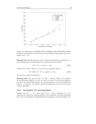
Example 3.2. Tables 3.2 and 3.3 show convergence results for Model Problem
1 as in Section 3.7 Example 3.1, obtained after the inclusion of a preconditioner
in the COCG, GMRES and Bi-CGSTAB algorithms. (Here we do not com-
pute the solution by CGNR). The preconditioners are ILU(0) and ILU( ) with
= 0.01 (thus, denoted by ILU(0.01)). We take kh = 0.625. Compared to the
unpreconditioned case, the use of ILU(0) and ILU(0.01) as preconditioners ac-
celerates the convergence significantly, with more fill-in, in general, giving faster
convergence for small wavenumber. For large wavenumber, for example k = 100,
all methods show a slow convergence, with ILU(0.01) becoming ineffective as
compared to ILU(0). Since A is not an M-matrix, an ILU factorization applied
to A is not a stable process. This may lead to an inaccurate LU approximation
of A, and, therefore, lead to a bad preconditioner for A.
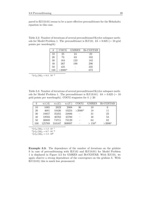
Different from the case without preconditioners, COCG turns out to con-
verge slower than the other methods, and does not converge (after 10,000 iter-
ations, Table 3.3) for high wavenumbers if ILU(0.01) is used as preconditioner.
This is because ILU(0.01) does not lead to a symmetric preconditioner. Thus,
the preconditioned linear system is not guaranteed to be symmetric. GMRES
and Bi-CGSTAB result in a comparable convergence in terms of the number of
iterations. As Bi-CGSTAB requires two matrix-vector products and two pre-
conditioner solves, the overall performance of Bi-CGSTAB is not better than
GMRES. GMRES may, however, suffer from storage problems if larger problems
(for an increasing k, as indicated by “–” in Table 3.2 for k = 50 and 100) have
to be solved, which tend to require too many iterations to reach convergence.
In Table 3.3 we measure the number of nonzero elements in the L and U
matrices for ILU(0.01). For increasing k, and thus N, the number of nonzero
elements becomes unacceptably large. ILU(0), which results in far less nonzero
elements (similar to the nonzero elements of A) in the L and U matrices com-](https://image.slidesharecdn.com/erlangga-160128071050/85/Erlangga-52-320.jpg)
![40 Krylov subspace iterative methods
0 10 20 30 40 50 60 70
0
50
100
150
200
250
Gridpoint per wavelength
No.Iterations
ILU(0)
ILU(0.01)
Figure 3.3: Performance (in number of iterations) of GMRES (dashed line)
and Bi-CGSTAB (solid line) for Model Problem 1 with respect to an increasing
number of grid points per wavelength. The upper part is for preconditioning
with ILU(0). The lower part is for ILU(0.01).
3.8.2 Incomplete factorization-based preconditioner
An ILU factorization may not be stable if A is not an M-matrix, which is the
case for the discrete Helmholtz equation. This is particularly observed from
numerical results in Section 3.8.1 with ILU(0.01) as preconditioner. In the
remainder of this chapter we discuss some preconditioners which are suitable
for the Helmholtz equation. Therefore, A should now be considered as a matrix
which is obtained from a discretization of the Helmholtz equation.
For the indefinite Helmholtz equation, various types of preconditioners have
been proposed. Evaluations of incomplete Cholesky factorization applied to
“less-indefinite” Helmholtz matrices are given in [69]. Reference [47] shows that
a parabolic factorization of the Helmholtz equation on a semi-discrete level can
be used as a preconditioner. Reference [81] proposes a separation-of-variables
technique to approximately factorize the linear system. The factorization is
exact for constant wavenumbers, but becomes somewhat cumbersome in the
presence of heterogeneities, that may even lead to divergence of the iterative
methods.
In [69] a modification of A is proposed such that ILU factorizations can be
constructed safely. For the approximation of A−1
, denoted by M−1
I , a constraint](https://image.slidesharecdn.com/erlangga-160128071050/85/Erlangga-54-320.jpg)
![3.8 Preconditioning 41
is set such that the preconditioned system AM−1
I is definite or “less indefinite”
than the original system. Here the term “indefiniteness” is related to the real
part of spectrum of the given linear system: one demands that Re σ(AM−1
I ) >
0 (or Re σ(AM−1
I ) < 0).
For A ∈ CN×N
, a matrix A can be extracted from A where the real part of
A is a non-singular symmetric M-matrix [101]. In the situation of interest here
(i.e., the Helmholtz equation discretized by the 5-point stencil), if one introduces
a parameter γ ≥ 1 and defines
Re(ai,j ) =
Re(ai,j) if i = j,
Re(ai,j) − γ min{0, Re((Ae)i)} if i = j,
it can be proven that Re(A) is a non-singular symmetric M-matrix [69]. Then,
Re(A) can be considered as a real perturbation of Re(A). Since Re(A) is a
symmetric M-matrix, ILU can be applied safely. For the imaginary part, one
simply sets
Im(aij) = Im(aij ), ∀i, j.
In [69] several possible strategies for this preconditioner are proposed. In
this thesis, we only describe one of them, namely
MI ≡ A = A0 + ˆjIm(A), A0 = Re(A) + Q, (3.30)
with
qii = − min{0, Re((Ae)i)}. (3.31)
We use (3.30)–(3.31) in Chapter 5, in combination with ILU(nlev), nlev = 0, 1.
Reference [69] evaluates the preconditioner for a finite element discretization of
the Helmholtz equation. In principle, one could also use a multigrid method for
approximating M−1
I , but since MI is constructed based on matrix modifications,
the multigrid method should preferably be an algebraic multigrid method (see,
for example, [92]).
3.8.3 Separation-of-variables preconditioner
It is well known that a separation of variables technique can be used to analyt-
ically solve the Laplace equation with special boundary conditions. The zeroth
order term k2
(x1, x2)u prevents the use of this technique in the same way for the
Helmholtz operator. An approximation can, however, be made in the separation
of variables context. This approximation can then be used as a preconditioner
for the Helmholtz equation.
For k2
(x1, x2) an arbitrary twice integrable function, the following decom-
position can be made,
k2
(x1, x2) = k2
x1
(x1) + k2
x2
(y) + ˜k2
(x1, x2), in Ω = [x1a , x1b
] × [x2a , x2b
],(3.32)](https://image.slidesharecdn.com/erlangga-160128071050/85/Erlangga-55-320.jpg)
![42 Krylov subspace iterative methods
satisfying the conditions
x1b
x1a
˜k2
(x1, x2)dx1 = 0, ∀x2,
x2b
x2a
˜k2
(x1, x2)dx2 = 0, ∀x1.
It can be proven that the decomposition (3.32) is unique [81]. Denoting by K,
a matrix representation of the zero-th order term, and L∆, the Laplace term,
matrix A can be written as
A = L∆ − K2
= X1 + X2 − K2
,
where
X1 = Ix2 ⊗ Ax1 , X2 = Ax2 ⊗ Ix1 , and K2
= Ix2 ⊗ K2
x1
+ K2
x2
⊗ Ix1 + K2,
with ⊗ the Kronecker product, Ix1 , Ix2 identity matrices and K2
x1
, K2
x2
, K2 di-
agonal matrices related to (3.32).
It is ˜k in (3.32) which prevents a complete decomposition of A. If we neglect
this term, K2
can be decomposed in the same way as L∆. This results in the
following separated variables formulation
A := X1 + X2 − K2 = Ix2 ⊗ (Ax1 − K2
x1
) + (Ax2 − K2
x2
) ⊗ Ix1 , (3.33)
where A approximates A up to the term K2. If wavenumber k is constant then
decomposition (3.32) is exact. As A can be further decomposed into a block
tridiagonal matrix, it is motivating to use A as a preconditioner for A. We
denote this preconditioner throughout this paper by MSV := A.
The construction of a block tridiagonal decomposition of MSV involves the
singular value decomposition in one direction, e.g. in the x1-direction. We refer
to [81] for more details.](https://image.slidesharecdn.com/erlangga-160128071050/85/Erlangga-56-320.jpg)
![Chapter 4
Shifted Laplace
preconditioner
We have seen in Chapter 3 that standard Krylov subspace methods converge
too slowly for the 2D Helmholtz equation. Furthermore, the convergence was
strongly dependent on the gridsize. Preconditioning based on an incomplete LU
factorization of the discrete Helmholtz equation does not effectively improve the
convergence for general cases. ILU(0.01) requires an unacceptably large storage,
but is still not effective in improving the convergence. ILU(0), on the other hand,
only requires a moderate storage. Its convergence is, however, not impressive
and sensitive to the gridsize.
In the last three decades efficient preconditioners for indefinite linear systems
have attracted attention of many researchers. The linear algebra theory for
indefinite linear systems, however, is not as well-developed as the theory for
definite linear systems.
For definite, elliptic boundary value problems, theoretical guidelines for pre-
conditioning are provided in [71] which justify the usual suggestion of choosing
the leading parts of an elliptic operator as the preconditioner. Reference [5]
analyzes preconditioners for an M-matrix, with the rate of convergence of the
conjugate gradient method given in [6]. For indefinite linear systems, theoretical
analysis of preconditioners can be found in [108]. Implementation of incomplete
factorization and block SSOR as preconditioners for indefinite problems is dis-
cussed in [45].
In [12],[51] and [64] preconditioners based on definite elliptic operators are
used in the context of Krylov subspace methods accelerated by multigrid.
Here we introduce a special class of preconditioners for the Helmholtz equa-
tion [37, 38, 102] to effectively improve the convergence of Krylov subspace
methods. This class of preconditioners is constructed by discretization of the
following operator
M(β1,β2) := −∆ − (β1 − ˆjβ2)k2
, β1, β2 ∈ R, (4.1)](https://image.slidesharecdn.com/erlangga-160128071050/85/Erlangga-57-320.jpg)
![44 Shifted Laplace preconditioner
which is called “shifted Laplace operator”. The preconditioners used in [12] and
[64] also belong to this class of preconditioners. They can be recovered from
(4.1) by setting (β1, β2) = (0, 0) and (β1, β2) = (−1, 0), respectively.
In this chapter we discuss the shifted Laplace preconditioner in detail. To
get insight in this class of preconditioners we first look at a 1D analysis for the
continuous operator with a “real” shift as used in [12] and [64], followed by a
purely “imaginary” shift (introduced in [37, 38]). Then, spectral analysis on
the discrete level is given in Section 4.2 under the restriction that the discrete
formulation of M(β1,β2) (4.1) should result in a (complex) symmetric, positive
definite matrix (CSPD). A convergence analysis which is based on the conver-
gence rate of GMRES is derived in Section 4.3. We then show in Section 4.4 that
the convergence is gridsize-independent. Some preliminary numerical results are
presented in Section 4.5, to show the effectiveness of this class of preconditioners
for a simple heterogeneous Helmholtz problem.
4.1 1D analysis for constant wavenumbers
In this section some analysis which motivates the development of the shifted
Laplace preconditioners is given. For simplicity and clarity we provide the anal-
ysis for the “undamped”, one-dimensional Helmholtz equation in this section.
Thus, α = 0 in (1.26).
4.1.1 Real shift
We consider here a 1D Helmholtz equation in a unit domain Ω = (0, 1):
−
d2
u
dx2
1
− k2
u = 0, (4.2)
with Dirichlet boundary conditions u(0) = u(1) = 0. For simplicity we only
consider problems with constant k over Ω. A non-trivial solution for the related
continuous eigenvalue problem
−
d2
dx2
1
+ k2
u = λu. (4.3)
is a general solution of the form u = sin(ax1). This solution satisfies the condi-
tions at x1 = 0 and x1 = 1. By substituting this solution in (4.3) we arrive at
the following relation:
(k2
1
− k2
) sin(π 1x1) = λ sin(π 1x1) → λ 1
= k2
1
− k2
, (4.4)
where k 1 = π 1, 1 ∈ N/{0}. Thus, for large wavenumbers k the eigenvalues
change sign, indicating the indefiniteness of the problem.
In 1D the preconditioning operator (4.1) reads
Mβ1 := −
d2
dx2
1
− β1k2
, with β ≤ 0. (4.5)](https://image.slidesharecdn.com/erlangga-160128071050/85/Erlangga-58-320.jpg)
![4.1 1D analysis for constant wavenumbers 45
We restrict ourselves to the preconditioning operator with β1 ≤ 0, since in this
case a finite difference discretization of (4.5) leads to a symmetric, positive defi-
nite matrix (SPD). Numerous efficient methods exist for solving such a matrix.
In particular, β1 = 0 and β1 = −1 give preconditioners used by Bayliss et al.
[12] and Laird et al. [64], respectively. In relation with the continuous eigenvalue
problem, the preconditioned (generalized) eigenvalue problem reads
−
d2
dx2
1
− k2
u 1
= λ 1
r −
d2
dx2
1
− β1k2
u 1
. (4.6)
By assuming a solution of the form u = sin(ax1), the eigenvalues are found
to be
λ 1
r =
k2
1
− k2
k2
1
− β1k2
=
1 − (k/k 1 )2
1 − β1(k/k 1 )2
, (4.7)
where k 1 = π 1, 1 ∈ N/{0}. For 1 → ∞, λ 1
r → 1, i.e., the eigenvalues are
bounded above by one. For 1 → 0, the low eigenmodes, we have λ 1
r → 1/β1.
The modulus of this eigenvalue remains bounded unless −1 ≤ β1 ≤ 0. The
maximum eigenvalue can therefore be written as
|(λ 1
r )max| = max
1
β1
, 1 . (4.8)
To estimate the smallest eigenvalue, we use a simple but rough analysis as
follows. It is assumed that the minimum eigenvalue is very close (but not equal)
to zero. This assumption implies a condition k 1 ≈ k as obtained from (4.7). To
be more precise, let k 1 = k + , where is any small number. By substituting
this relation into (4.7), and by neglecting the higher order terms and assuming
that k k2
, we find that
(λ 1
r )min =
2
1 − β1 k
. (4.9)
From (4.9), the minimum eigenvalue can be very close to zero as β1 goes to
infinity. The condition number of the preconditioned Helmholtz operator now
reads
κ =
1
2 (1 − β1)k/ if β1 ≤ −1,
1
2|β1| (1 − β1)k/ if − 1 ≤ β1 ≤ 0.
(4.10)
If β1 ≤ −1, κ is a monotonically increasing function with respect to |β1|.
The best choice is β1 = −1, which gives the minimal κ in this context. If
−1 ≤ β1 ≤ 0, κ is a monotonically increasing function with respect to β1. κ is
minimal in this range if β1 = −1. In the limit we find that
lim
β1↓−1
κ = lim
β2↑−1
κ = k/ , (4.11)](https://image.slidesharecdn.com/erlangga-160128071050/85/Erlangga-59-320.jpg)
![46 Shifted Laplace preconditioner
−6 −5 −4 −3 −2 −1 0
0
0.5
1
1.5
2
2.5
3
3.5
4
β
1
κεk
−1
Figure 4.1: Condition number κ of M−1
A vs. coefficient β1 for the real shifted
Laplace preconditioner
which is the minimum value of κ for β1 ≤ 0 ∈ R (see Figure 4.1).
The relation (4.10) tells us that taking the leading part of the Helmholtz
equation (i.e. the Laplacian term, β1 = 0) is generally advisable for high
wavenumbers, as advocated in [71]. However, this is no longer true for small
wavenumbers, for which the condition number of the preconditioned linear sys-
tem may become very large. From the convergence bound of CG (3.18) the
result (4.10) also gives an indication that setting β1 = −1 in (4.5) leads to a
fast converging preconditioned iterative method for the Helmholtz equation.
4.1.2 Generalization to complex shift
The basic analysis on 1D shifted Laplace preconditioners for β1 ≤ 0 in Sec-
tion 4.1.1 gives β1 = −1 as the optimum case. A nice property of the real
shifted Laplace operator, at least in 1D, is that the eigenvalues have an upper
bound. However, this property does not guarantee that the eigenvalues are fa-
vorably distributed. There is the possibility that one or more eigenvalues lie
very close to zero. For example, setting β1 = −1 gives the minimal condition
number κ but, at the same time, results in λmin which is not better than for
β1 = 0. We can improve the preconditioner by preserving the boundedness and
at the same time shifting the minimum eigenvalue as far as possible from zero.
Consider the minimum eigenvalue λmin obtained from the 1D problem (4.2).
We may shift this eigenvalue away from zero by adding some real value to λ.
In general, this addition will shift all eigenvalues, which is undesirable. An
alternative is to multiply the eigenvalues by a factor. From (4.7) the relation](https://image.slidesharecdn.com/erlangga-160128071050/85/Erlangga-60-320.jpg)
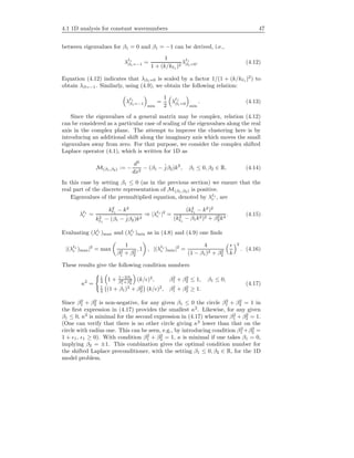
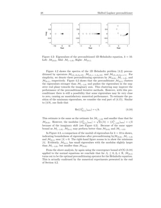
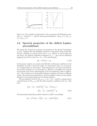
![50 Shifted Laplace preconditioner
with uh the eigenvector corresponding to the discrete eigenvalue λ.
Both systems (4.19) and (4.20) are indefinite if k2
is larger than the smallest
eigenvalue of Lh. In this case, the convergence properties of (4.20) are difficult
to estimate. Therefore, for analysis purposes the subsequent analysis will be
based on a normal equations formulation of the preconditioned matrix system
(as in [64]).
Denote the ordered eigenvalues of Lh as 0 < µ1 ≤ · · · ≤ µN , and the normal
equations A∗
hAh, (M−1
h,(0,0)Ah)∗
(M−1
h,(0,0)Ah), (M−1
h,(−1,0)Ah)∗
(M−1
h,(−1,0)Ah) and
(M−1
h,(0,1)Ah)∗
(M−1
h,(0,1)Ah) as QA, Q(0,0), Q(−1,0) and Q(0,1), respectively. We
find the eigenvalues in the four following cases as:
λ (QA) = µm − k2 2
, (4.22)
λ Q(0,0) =
µm − k2
µm
2
= 1 −
k2
µm
2
, (4.23)
λ Q(−1,0) =
µm − k2
µm + k2
2
= 1 −
2k2
µm + k2
2
, (4.24)
λ Q(0,1) =
µm − k2
µm + ˆjk2
µm − k2
µm + ˆjk2
= 1 −
2µmk2
µ2
m + k4
. (4.25)
We first consider the case where k is small such that 0 < k2
< µ1, where µ1
the smallest eigenvalue of −Lh. Using (4.22)–(4.25), we find the minimal and
maximal eigenvalues as follows:
λ (QA)min = µ1 − k2 2
, λ (QA)max = µN − k2 2
,
λ Q(0,0) min
= 1 −
k2
µ1
2
, λ Q(0,0) max
= 1 −
k2
µN
2
,
λ Q(−1,0) min
= 1 −
2k2
µ1 + k2
2
, λ Q(−1,0) max
= 1 −
2k2
µN + k2
2
,
λ Q(0,1) min
= 1 −
2µ1k2
µ2
1 + k4
, λ Q(0,1) max
= 1 −
2µN k2
µ2
N + k4
.
Since k2
/µ1 < 1, one easily sees that
λ Q(0,0) min
> λ Q(−1,0) min
.
As m → ∞, one finds also that
lim
µN →∞
λ Q(0,0) max
= lim
µN →∞
λ Q(−1,0) max
= 1.
With respect to the l2-condition number, it becomes evident that for k <
√
µ1,
preconditioning with Mh,(0,0) gives a lower condition number than precondition-
ing with Mh,(−1,0). Hence, for small k, Mh,(0,0) is more effective than Mh,(−1,0).](https://image.slidesharecdn.com/erlangga-160128071050/85/Erlangga-64-320.jpg)
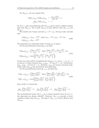
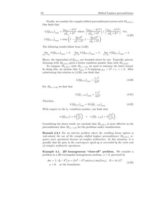
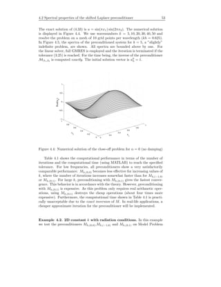
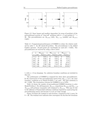
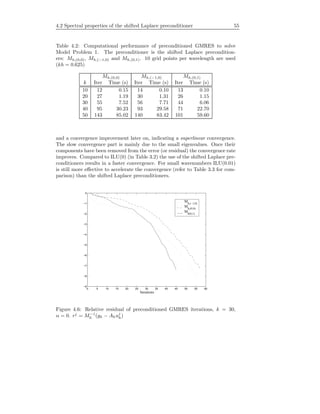
![56 Shifted Laplace preconditioner
4.3 Bound of convergence rate of GMRES
In this section we apply GMRES convergence analysis for the discrete 2D
Helmholtz equation, preconditioned by the shifted Laplace preconditioner. In
particular, we consider Mh,(0,1) as the preconditioner. We first provide the
spectral properties of a Helmholtz problem with Dirichlet boundary conditions
(which is called “closed-off problem”). In Section 4.3.2, we use the results to ob-
tain a bound for the GMRES convergence rate with radiation conditions (2.26).
Again, for simplicity we set wavenumber k to be constant over Ω, and α = 0
(undamped). We have presented these results in [40].
4.3.1 Closed-off problem
The two-dimensional, “closed-off” Helmholtz problem to be analyzed is defined
as follows:
Au := −
∂2
u
∂x2
1
−
∂2
u
∂x2
2
− k2
u = 0, in Ω = (0, 1)2
, (4.34)
u(0, x2) = u(1, x2) = 0, u(x1, 0) = u(x1, 1) = 0. (4.35)
The eigenvalue problem related to (4.34)–(4.35) reads
−
∂2
∂x2
−
∂2
∂y2
− k2
u 1, 2
= λ 1, 2
u 1, 2
, 1, 2 ∈ N (4.36)
u 1, 2
(0, x2) = u 1, 2
(1, x2) = 0, (4.37)
u 1, 2
(x1, 0) = u 1, 2
(x1, 1) = 0, (4.38)
where u 1, 2
and λ 1 2
are the eigenfunctions and eigenvalues, respectively. The
eigenfunctions
u 1, 2
= sin( 1πx) sin( 2πy), for 1, 2 ∈ N. (4.39)
satisfy (4.36)-(4.38). Substituting these eigenfunctions in (4.36) yields
λ 1, 2
= k2
1
+ k2
2
− k2
, k 1 = 1π, k 2 = 2π. (4.40)
In this case k 1 , k 2 are the natural frequencies. Resonance occurs if the
wavenumber (or reduced frequency), k, is equal to k 1 2 := k2
1
+ k2
2
. It
resembles the condition λ 1, 2
= 0.
Now, the complex shifted Laplace preconditioner M(0,1) in 2D is used to
speed up the convergence. We can write the preconditioned eigenvalue problem
as
−
∂2
∂x2
1
+
∂2
∂x2
2
+ k2
u 1, 2
= λ 1, 2
p −
∂2
∂x2
1
−
∂2
∂x2
2
+ ˆjk2
u 1, 2
. (4.41)](https://image.slidesharecdn.com/erlangga-160128071050/85/Erlangga-70-320.jpg)
![58 Shifted Laplace preconditioner
Re
Im
Im
Re
θ
θ
θ
Figure 4.7: Rotation of the z-plane.
or
λ 1, 2
p,− π
4
−
1
2
√
2 =
1
2
√
2, (4.50)
which leads to the following lemma.
Lemma 4.3.2 Let the 2D Helmholtz problem (4.34) with boundary conditions
(4.35) be preconditioned by M(0,1) and assume that resonance does not occur.
Furthermore, let the spectrum be rotated according to (4.44). For θ = −π/4,
the spectrum has the following properties:
(i) All eigenvalues lie on a circle with center zc,−π
4
= 1
2
√
2 and radius r =
1
2
√
2. There are no zero eigenvalues.
(ii) This circle is independent of wavenumber k.
Figure 4.8 illustrates Lemma 4.3.2, for k = 10. The grid size affects the
position of the small eigenvalues, which asymptotically move closer to the origin.
As the circle contains the origin, the classical convergence bound for GMRES
cannot be used to estimate the convergence. Therefore, a closer look at the
eigenvalues in the vicinity of the origin is required, if one wants to estimate the
rate of convergence. On the other hand, the result implies that if an eigenvalue
close to the origin is well approximated by a Ritz value during the GMRES
process, the convergence of GMRES becomes superlinear [99], which is indeed
observed in our numerical experiments in Section 4.2 (see Figure 4.6).
From Lemma 4.3.2, we get the following corollary.
Corollary 4.3.3 Let the 2D Helmholtz problem (4.34) with boundary conditions
(4.35) be preconditioned by operator M(0,1). Then, the spectrum lies on the
circle |z − zc| = 1
2
√
2, with zc = 1
2 (1 + ˆj) the center of circle.
Proof The proof can be obtained by back transformation of the result in
Lemma 4.3.2 by using the rotation matrix (4.44) with θ = π/4.](https://image.slidesharecdn.com/erlangga-160128071050/85/Erlangga-72-320.jpg)
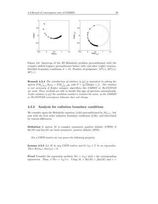
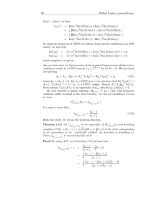
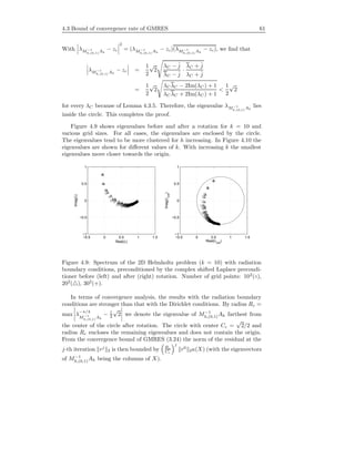
![4.5 Extension to heterogeneous media 63
where |µc
m −k2
| = min 1 |µc
1
−k2
|. Combining this limit with the analysis given
in Section 4.2, for Mh,(0,1) we can show that [102]
lim
h→0
λmin(Q(0,1)) =
|µc
m − k2
|2
2k4
. (4.55)
Since the maximal eigenvalues of Q(0,1) are bounded by 1, we conclude that the
convergence behavior of this preconditioners is independent of h (see also [71]).
Only initially there can be dependence of the smallest eigenvalue on h. In a
similar way, for Mh,(−1,0) we find that
lim
h→0
λmin(Q(1,0)) =
|µc
m − k2
|2
4k4
, (4.56)
which also indicates an h-independent convergence.
Example 4.3. h-independence convergence. To show the convergence be-
havior with respect to the gridsize, h, we consider the problem described in
Example 4.1 and solve it on different gridsizes using GMRES. The convergence
results are shown in Table 4.3 and confirm the h-independent convergence be-
havior. Similar results are obtained for Bi-CGSTAB.
Table 4.3: Computational performance of GMRES (in terms of number of it-
erations) to solve the “close-off” problem (see Example 4.1) with different grid
resolutions
Mh,(0,0) Mh,(−1,0) Mh,(0,1)
h−1
h−1
h−1
k 50 100 150 50 100 150 50 100 150
10 13 14 14 17 17 17 15 15 16
20 26 26 28 29 30 32 25 26 26
30 52 57 57 54 59 60 44 47 49
40 99 96 98 96 96 99 79 78 80
4.5 Extension to heterogeneous media
In the analysis and numerical tests given so far, we only treated problems in
homogeneous media. In real applications we typically encounter problems with
heterogeneous properties of the media. Extension of the method to problems
with heterogeneity is straightforward. The analysis, however, is much harder.
Example 4.4. Three-layer problems. We show numerical results for a 2D
problem in Ω = (0, 1)2
with three layers wherein a simple heterogeneity in k is](https://image.slidesharecdn.com/erlangga-160128071050/85/Erlangga-77-320.jpg)
![4.5 Extension to heterogeneous media 65
From Table 4.4, we also see that preconditioned Bi-CGSTAB does not per-
form well for Mh,(0,0) and Mh,(−1,0), as already indicated in [64], but per-
forms satisfactorily for Mh,(0,1), with a comparable performance as compared
to COCG (in terms of matrix/vector multiplications). Compared to GMRES,
Bi-CGSTAB and COCG preconditioned by Mh,(0,1) show a better convergence
performance for increasing wavenumbers (despite the fact that Bi-CGSTAB
requires two preconditioning steps per iteration). If Mh,(0,1) is used as the pre-
conditioner, Bi-CGSTAB and COCG can replace full GMRES.
From Table 4.4, one also concludes that CGNR may not be a good iterative
method to solve the Helmholtz problem with the shifted Laplace precondition-
ers. This is due to the squaring of the original eigenvalues in the case of the
normal equations, causing too many small eigenvalues. With such a spectrum,
CG-type methods often exhibit very slow convergence. However, since our anal-
ysis for the preconditioners is based on the normal equations, the results of
CGNR are included and are in accordance with the analysis with respect to
other preconditioners.](https://image.slidesharecdn.com/erlangga-160128071050/85/Erlangga-79-320.jpg)

![Chapter 5
Multigrid for the
preconditioner solve
In the previous chapter we have shown that for high wavenumbers the shifted
Laplace preconditioners were able to effectively accelerate the convergence of
Krylov subspace methods. Furthermore, we have also shown that the shifted
Laplace preconditioner with an imaginary shift, denoted by Mh,(0,1), leads to
the preferred choice. Therefore, for the time being, we will restrict ourselves to
a purely complex symmetric, positive definite (CSPD) preconditioner. In Chap-
ter 6, we will loosen this requirement. We have also shown that the convergence
of the preconditioned Krylov subspace method (in that case GMRES) is inde-
pendent of gridsize h. In the numerical examples that are given in Chapter 4
we have used, however, a direct solution method to invert the preconditioner in
the Krylov subspace method algorithms. This is too expensive, and even more
expensive than solving the original problem.
There exist methods to efficiently solve a CSPD system. One idea is to solve
the preconditioner by means of other iterative methods. One of the techniques
is by using GMRESR [99], which combines GCR as the outer iteration with
GMRES as the inner iteration. This algorithm is, however, expensive in actual
tests if compared with Bi-CGSTAB. An attractive approach is to approximately
solve the preconditioner by using multigrid [20, 53, 92, 105].
Multigrid is known for its efficiency and robustness when it is applied to a
discrete elliptic operator. A multigrid method exhibits fast convergence inde-
pendent of gridsize, h, and with a complexity of O(N log N). To achieve such a
convergence, however, requires a careful design involving many components in
a multigrid method.
This chapter deals with multigrid for solving the preconditioner in the pre-
conditioned Krylov subspace method. We first discuss the principles of multigrid
methods and the actual implementation of these principles. We then explain in
Section 5.2 why the application of multigrid directly to the Helmholtz equation
leads to convergence difficulties. In Section 5.4 we review Fourier analysis which](https://image.slidesharecdn.com/erlangga-160128071050/85/Erlangga-81-320.jpg)
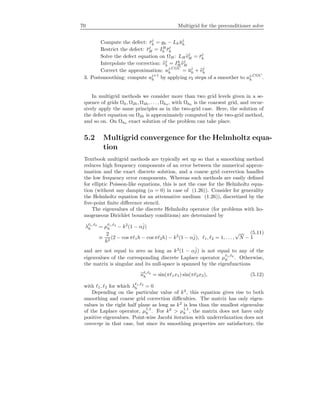
![5.3 Multigrid components 71
multigrid convergence will deteriorate only gradually for k2
increasing. By the
time k2
approaches the 6th eigenvalue µ 1, 2
h (k2
≈ 150), standard multigrid
diverges. The Jacobi relaxation now diverges for smooth eigenfrequencies u 1, 2
h
with µ 1, 2
h < k2
. Consequently, multigrid will still converge as long as the
coarsest level used is fine enough to represent these smooth eigenfrequencies
sufficiently. So, the coarsest level chosen limits the convergence. When k2
gets
larger more variables need to be represented on the coarsest level for standard
multigrid convergence. Eventually, this does not result in an O(N log N) itera-
tive method.
In addition to this feature, the Helmholtz equation also brings a multigrid
coarse grid correction difficulty. Eigenvalues close to the origin may undergo a
sign change after discretization on a coarser grid. If a sign change occurs the
coarse grid solution does not give a convergence acceleration to the finer grid
problem, but a severe convergence degradation (or even divergence) instead.
In [33] this phenomenon is analyzed and a remedy for the coarse grid correction
related to these problematic eigenvalues is proposed. The efficient treatment
in [33] is that multigrid is combined with Krylov subspace iteration methods.
GMRES is proposed as a smoother and as a cure for the problematic coarse grid
correction. The convergence results achieved are impressive.
Standard multigrid will also fail for k2
-values very close to eigenvalues. In
that case subspace correction techniques should be employed [23].
An advanced multigrid based solution method for the Helmholtz equation is
the wave-ray multigrid method [22]. The method has been adapted for a first-
order system least-squares version of the Helmholtz equation in [65]. Wave-ray
multigrid has been developed for Helmholtz problems with constant or smoothly
varying wavenumbers. A thorough overview for the numerical solution of the
Helmholtz equation is presented in [94].
5.3 Multigrid components
In this section, we detail the multigrid components that can be specified for
approximately inverting a discrete version of the preconditioning operator M
(4.1). We consider the 5-point discretization and denote the discrete precondi-
tioner as Mh. Furthermore, we consider the right preconditioned system. Thus,
we solve the equivalent system
AhM−1
h wh = gh, Mhuh = wh, (5.13)
with Mhuh = wh solved by one multigrid iteration. Standard multigrid coars-
ening, i.e., doubling the mesh size h in every direction is chosen. Since we are
now applying multigrid to Mh, the discrete operator Lh (and LH ) in Algorithm
4.1 are replaced by Mh (and MH).](https://image.slidesharecdn.com/erlangga-160128071050/85/Erlangga-85-320.jpg)
![72 Multigrid for the preconditioner solve
5.3.1 Smoothers
Classical iteration methods like Jacobi with underrelaxation and Gauss-Seidel
iterations can be used as smoothers. We denote the two smoothers by ωr-
JAC and ωr-GS, respectively. In principle one can choose the underrelaxation
parameter ωr ∈ C, but the Fourier analysis (discussed in Section 5.4) indicates
that there is no real benefit for the problems considered later in this chapter
and in Chapter 6. So, we choose ωr ∈ R.
For the Poisson equation, setting ωr = 1 in Jacobi smoother does not lead
to an iterative method with smoothing properties. For Gauss-Seidel, ωr = 1 al-
ready results in good smoothing in combination with lexicographical ordering.
This smoothing property improves if red-black ordering is used. We denote the
Gauss-Seidel relaxation with red-black ordering by ωr-GS-RB. Fourier smooth-
ing analysis of these two relaxation methods is explained in [92].
5.3.2 Prolongation and restriction operators
For the intergrid transfer of the grid functions two (linear) transfer operators
(5.8) and (5.9) are required. There are several ways to construct the transfer
operators.
A frequently used prolongation operator is based on bilinear interpolation
(denoted by BI) from GH to Gh. This interpolation is defined as (see Figure 5.1)
Ih
H vH (x, y) =
vH (x, y) for A
1
2 [vH (x1, x2 + h) + vH (x1, x2 − h)] for q
1
2 [vH (x1 + h, x2) + vH (x1 − h, x2)] for p
1
4 [vH (x1 + h, x2 + h) + vH (x1 + h, x2 − h)
+vH (x1 − h, x2 + h) + vH (x1 − h, x2 − h) for r
(5.14)
We also consider a prolongation operator which is based on operator-dependent
interpolation (denoted by MD) based on de Zeeuw’s transfer operators [109], for
example, for heterogeneous Helmholtz problems. Originally, this prolongation
was set up for general (possibly unsymmetric) real-valued matrices with a split-
ting of matrix M into a symmetric and an antisymmetric part, see [109]
Mh,s =
1
2
(Mh + MT
h ), Mh,t = Mh − Mh,s.
However, since the discretization here leads to a complex symmetric matrix,
the prolongation is adapted and briefly explained for such matrices with nine
diagonals [35].
The notation in a stencil for the explanation of the prolongation is as in
Figure 5.2 (left side). The right picture in Figure 5.2 shows one coarse and
four fine grid cells with indices for the explanation of the interpolation weights.
Capital letters denote coarse grid, lower case letters fine grid points. Operator
element mw
p , for example, denotes the west element of operator Mh at point p
on the fine grid.](https://image.slidesharecdn.com/erlangga-160128071050/85/Erlangga-86-320.jpg)

![74 Multigrid for the preconditioner solve
• for fine grid points q in Fig. 5.2: eh,q = wAeH,A + wCeH,C.
wA = min(1, max(0, ws)); wC = min(1, max(0, wn)),
with
dn = max(|mnw
q + mn
q + mne
q |, |mnw
q |, |mne
q |) (5.18)
ds = max(|msw
q + ms
q + mse
q |, |msw
q |, |mse
q |) (5.19)
ws =
ds
ds + dn
, wn =
dn
ds + dn
(5.20)
On the remaining points the prolongation is defined as follows
• On fine grid points that are also coarse points: eh(A) = eH (A)
• On points r: eh(r) is determined so that MhIh
H eH = 0 at r.
The interpolation weights are the same as in [109], but especially tailored
to the symmetric complex Helmholtz equation. |.| denotes the modulus, in
this case. As for symmetric problems with jumping coefficients, the prolon-
gation operator by de Zeeuw [109] is very similar to the original operator-
dependent prolongation in [3] and [62]. In [3], for dw, for example, the lumped
sum of three elements, msw
p + mw
p + mnw
p is chosen. For satisfactory conver-
gence it is, however, important to use the modulus of the operator elements, as
in (5.15), (5.16), (5.18),(5.19) in the definition of the interpolation weights.
For the restriction, the simplest choice is injecting the value on a fine grid
points to the corresponding coarse grid points. This is called injection. A
commonly used restriction operator is called the full weighting (FW) operator,
which can be considered as a nine-point weighted average of a (fine) grid function
on a coarse grid. For full weighting, the restriction operator reads
dH (x1, x2) = IH
h dh(x1, x2)
=
1
16
[4dh(x1, x2) + 2dh(x1 + h, x2) + 2dh(x1 − h, x2)
+ 2dh(x1, x2 + h) + 2dh(x1, x2 − h) + dh(x1 + h, x2 + h)
+ dh(x1 − h, x2 + h) + dh(x1 + h, x2 − h) + dh(x1 − h, x2 − h)],
(5.21)
or, in stencil notation,
IH
h =
1
16
1 2 1
2 4 2
1 2 1
H
h
. (5.22)
In general, we do not choose for the adjoint of the prolongation operator,
which is commonly used but not absolutely necessary (as already stated in [3]
and an example where the restriction is not the adjoint of the prolongation
operator has been given in [30]), unless a combination of bilinear interpolation
and full weighting is evaluated. In this case the adjoint of bilinear interpola-
tion operator equals the full weighting operator. Choosing the combination of a](https://image.slidesharecdn.com/erlangga-160128071050/85/Erlangga-88-320.jpg)
![5.4 Fourier analysis 75
full weighting restriction and the operator-dependent interpolation brings to a
robust convergence for a variety of Helmholtz problems with constant and non-
constant coefficients. For constant coefficients and mildly varying wavenumbers,
bilinear interpolation (in combination with full weighting) also gives very sat-
isfactory convergence results, but for strongly varying coefficients, as in Model
Problem 3: the Marmousi problem, a robust and efficient convergence on differ-
ent grid sizes and for many frequencies is observed for the combination of the
transfer operators chosen.
5.3.3 Coarse grid operator, multigrid cycle
A natural choice for the coarse grid operator is to use a direct discretization of
the partial differential operator on the coarse grid ΩH . A different approach is
found in the so-called Galerkin coarse grid operator, which is defined by
M2h := I2h
h MhIh
2h, M4h := I4h
2h M2hI2h
4h , etc. (5.23)
In the Fourier analysis results in Chapter 6, this discretization is compared to a
direct coarse grid discretization of M. The Galerkin coarse grid discretization
seems a natural choice for heterogeneous problems. Also with boundary con-
ditions containing first and second derivatives it is more convenient to choose
the Galerkin coarse grid discretization, as it defines the appropriate coarse grid
boundary stencils automatically. The transfer operators in building the coarse
grid operators are the same as those used for transferring coarse and fine grid
quantities to fine and coarse grids, respectively.
In a two-grid method, we have only one possibility of how the sequence of
a fine and coarse grid is visited. As the number of grid levels increases, there
are many scenarios to process the grids. One typically distinguishes the V-,
F- and W-cycles, as depicted in Figure 5.3. On every visit a number of pre-
and postsmoothing steps is applied. By using the notation of Algorithm 4.1.
V(ν1,ν2), for example, means a V-cycle multigrid with ν1 steps of presmoothing
and ν2 steps of postsmoothing.
5.4 Fourier analysis
In this section we provide analysis for the multigrid convergence of the dis-
crete preconditioning operator Mh. There are several approaches to analyze the
multigrid convergence. For example, Hackbusch [53] gives analysis of multigrid
based on the approximation and smoothing properties of a multigrid method.
This approach gives, though important, qualitative results. On the other hand,
we are interested in quantitative estimates of the multigrid convergence. The
two-grid Rigorous Fourier Analysis (RFA) [92] is the primary tool in our multi-
grid analysis.](https://image.slidesharecdn.com/erlangga-160128071050/85/Erlangga-89-320.jpg)
![76 Multigrid for the preconditioner solve
Ω
Ω
Ω
Ω
h
2h
4h
8h
(i) (ii) (iii)
Multigrid with four grid levelsTwo−grid
Figure 5.3: Two- and multigrid cycle: (i) V-cycle, (ii) F-cycle and (iii) W-cycle
5.4.1 Two- and three-grid convergence analysis
Fourier smoothing and two-grid analysis, two classical multigrid analysis tools,
have been used for quantitative estimates of the smoothing properties and of the
other multigrid components in a two-grid method [19, 20, 21, 89, 92]. Consider
Mhuh = wh in (5.13), where uh represents the exact discrete solution. The
error vj
h = uj
h − uh after the j-th iteration is transformed by a two-grid cycle as
follows:
vj+1
h = T2h
h vj
h, T2h
h = Sν2
h K2h
h Sν1
h , K2h
h = Ih − Ih
2h(M2h)−1
I2h
h Mh. (5.24)
Mh, M2h correspond to discretizations of M on the h-, 2h-grid, Sh is the smooth-
ing operator on the fine grid, Ih the identity operator. ν1 and ν2 represent re-
spectively the number of pre- and postsmoothing steps, I2h
h and Ih
2h denote the
restriction and prolongation operator, respectively. In the analysis we assume
an equidistant grid with
√
N points in each direction.
The O(h2
) discrete complex Helmholtz operator from M belongs to the class
of symmetric stencils. For these stencils it is possible to apply Fourier analysis
on the basis of discrete sine-eigenfunctions φ 1, 2
h , 1, 2 = 1, . . . ,
√
N − 1 (5.3),
instead of the local Fourier analysis with exponential functions. For problems
with symmetric stencils and homogeneous Dirichlet boundary conditions, this
analysis can predict h-dependent convergence factors. (The definition of the
operator-dependent prolongation and the Galerkin coarse grid stencils in Sec-
tion 5.3.2 also lead to symmetric operators, that can be analyzed within this
framework.) From the discussion of multigrid for the original Helmholtz equa-
tion it seems necessary to gain insight into the h-dependency of the multigrid
methods developed also for the complex Helmholtz operator.
For the point-wise Jacobi smoother, the φ 1 2
h (5.3) are also eigenfunctions of
the smoothing operator. This is not true for Gauss-Seidel smoother and the two-
grid iteration operator T 2h
h . However, the 4-dimensional linearly independent](https://image.slidesharecdn.com/erlangga-160128071050/85/Erlangga-90-320.jpg)
![5.4 Fourier analysis 77
spaces, the harmonics:
E 1, 2
h = φ 1, 2
h , φ
√
N− 1,
√
N− 2
h , −φ
√
N− 1, 2
h , −φ 1,
√
N− 2
h (5.25)
for 1, 2 = 1, . . . ,
√
N
2 are invariant under these operators. One can show [89, 92]
that
Mh : span [φ 1, 2
h ] → span [φ 1, 2
h ], (M2h)−1
: span [φ 1, 2
2h ] → span [φ 1, 2
2h ],
Sh : span [φ 1, 2
h ] → span [φ 1, 2
h ],
I2h
h : E 1, 2
h → span [φ 1, 2
2h ], Ih
2h : span [φ 1, 2
2h ] → E 1, 2
h ,
and T2h
h : E 1, 2
h → E 1, 2
h ( 1, 2 = 1, ...,
√
N
2 ). Therefore, the representation of
T2h
h with respect to E 1, 2
h leads to a block-diagonal matrix, T2h
h ,
T2h
h
∧
= T2h
h ( 1, 2)
1, 2=1,...,
√
N
2
=: T2h
h . (5.26)
Here the blocks T2h
h ( 1, 2) are 4 × 4 matrices if 1, 2 <
√
N
2 , 2 × 2 (1 × 1)
matrices if either 1 =
√
N
2 or 2 =
√
N
2 ( 1 =
√
N
2 and 2 =
√
N
2 ). The two-grid
convergence factor is defined as
ρ2g := max
1≤ 1, 2≤
√
N
2
ρ T2h
h ( 1, 2) . (5.27)
Thus, the spectral radii of at most 4 × 4 matrices T2h
h ( 1, 2) have to be deter-
mined, and their maximum with respect to 1 and 2 has to be found.
The definition of the smoothing factor µ is closely related. The smoothing
factor measures the reduction of high frequency error components by an itera-
tive method. It is based on a coarse grid correction operator that annihilates
the low frequency error components completely and keeps the high frequency
components unchanged. K2h
h is replaced by a projection operator Q2h
h mapping
onto the space of high frequencies, i.e., a block diagonal matrix with Q2h
h at most
4 × 4-diagonal blocks defined by diag(0, 1, 1, 1). So, µ is computed as ρ2g (5.27)
with K2h
h in T2h
h replaced by Q2h
h .
Recently, three-grid Fourier analysis is proposed in [106]. An issue that can
be analyzed in some more detail with a third grid is the coarse grid correction.
If a large difference occurs between the two-grid and the three-grid convergence
factors, ρ2g and ρ3g, this is an indication for a problematic coarse grid correction.
For the complex Helmholtz preconditioner it seems important to analyze the
coarse grid correction carefully. The error transformation by a three-grid cycle
is given by
vj+1
h = T4h
h vj
h with
(5.28)
T4h
h = Sν2
h K4h
h Sν1
h and K4h
h = Ih − Ih
2h(I2h − (T4h
2h )γ
)(M2h)−1
I2h
h Mh.](https://image.slidesharecdn.com/erlangga-160128071050/85/Erlangga-91-320.jpg)
![78 Multigrid for the preconditioner solve
Here T4h
2h , defined by (5.24), reads T 4h
2h = Sν2
2h(I2h − I2h
4h (M4h)−1
I2h
4h )Sν1
2h. The
matrix M4h corresponds to 4h-grid discretization of M, S2h is the smoothing
operator and I2h the identity on the 2h-grid, I4h
2h and I2h
4h are transfer opera-
tors between the different grids. The 2h-equation is solved approximately in a
three-grid cycle (5.28) by performing γ two-grid iterations T 4h
2h with zero initial
approximation, see also [89, 106].
The three-grid analysis is a recursive application of the two-grid analysis.
Not only in the transition from h- to 2h-grid but also in the transition from
the 2h- to the 4h-grid, four frequencies are coupled. Thus the three-grid error
transformation operator couples 16 Fourier frequencies. As a consequence, T 4h
h
is unitarily equivalent to a block diagonal matrix T4h
h with at most 16 × 16
blocks, T4h
h ( 1, 2). The block matrices are composed of the Fourier symbols
from the two-grid analysis, which is due to the recursive application of the
two-grid analysis. One may compute the three-grid factor ρ3g, as the supre-
mum of the spectral radii from the 16 × 16 block matrices, T4h
h ( 1, 2). For
more details about the three-grid analysis, we refer to [106]. Three-grid Fourier
analysis software, based on the exponential functions, is freely available, see
www.mgnet.org/mgnet-codes-wienands.html.
5.4.2 Fourier analysis applied to the preconditioner with
imaginary shift
In this section we focus on the shifted Laplace operator with an imaginary shift:
M(0,1) := −∆ + ˆjk2
, (5.29)
and apply RFA to its discrete version Mh,(0,1).
We first consider multigrid with a V-cycle and ωr-GS-RB relaxation with
ωr = 1, which is a well-known combination for the Poisson equation. We set
k = 100 in (5.29), with kh = 0.625. The coarse grid matrices are constructed by
the Galerkin coarse grid discretization. Table 5.1 shows RFA results for this pre-
conditioning operator. In the table we show the two- and three-grid convergence
factor, ρ2g and ρ3g respectively, and the numerical multigrid convergence, ρh.
In addition, we compute the two-grid operator norm T 2h
h S = ρ(T2h
h (T2h
h )∗)
and the three-grid operator norm T 4h
2h S = ρ(T4h
2h (T4h
2h )∗), to quantify an
upper bound for the error reduction in only one multigrid iteration. This lat-
ter quantity is interesting since the method is used as a preconditioner and
only one multigrid iteration is applied for preconditioner solves in the Krylov
subspace methods. Here we have used the MD-FW transfer operators. The
matrix-dependent prolongation operator may be particularly important if a het-
erogeneity is present in the medium. For constant k the multigrid convergence
with this combination resembles that of the bilinear interpolation prolongation
operator. The V(1,0)-cycle is compared to V(1,1), where in parentheses the
number of pre- and post-smoothing steps are indicated. From RFA, the asymp-
totic two-grid convergence factor for the V(1,1)-cycle is about 0.06, which is in](https://image.slidesharecdn.com/erlangga-160128071050/85/Erlangga-92-320.jpg)
![5.4 Fourier analysis 79
a good agreement with the numerical convergence. Furthermore, the norm of
the two-grid operator is well below 0.2. Multigrid for (5.29) behaves very simi-
larly to the definite real version of the Helmholtz operator (and of the Laplace
operator).
Table 5.1: Comparison of asymptotic convergence from Fourier analysis with
numerical multigrid convergence, Mh,(0,1). µ is the smoothing factor; ρ2g, ρ3g
are the two- and three-grid convergence factor from Fourier analysis; ρh is the
numerical multigrid convergence factor. The smoother is ωr-RB-GS with ωr = 1
µ ρ2g T2h
h S ρ3g T4h
2h S ρh, V-cycle
V(1,0) 0.25 0.25 0.56 0.24 0.56 0.235
V(1,1) 0.06 0.06 0.14 0.06 0.14 0.055
We have also analyzed multigrid with γ = 2 and the ωr-JAC smoother,
applied to (5.29). Notice that for γ = 2 the F-cycle is identical to the W-cycle.
Underrelaxation parameter ωr is set to ωr = 0.8, as this is the optimal choice for
the Laplace operator [92]. Again, the agreement between the smoothing, two-
and three-grid Fourier analysis results with one and two smoothing iterations
and the numerical convergence is excellent, as presented in Table 5.2. The results
obtained are very similar to the convergence factors for the Laplace operator
with ωr-JAC.
Table 5.2: Comparison of asymptotic convergence from Fourier analysis with
numerical multigrid convergence, Mh,(0,1). µ is the smoothing factor; ρ2g, ρ3g
are the two- and three-grid convergence factor from Fourier analysis; ρh is the
numerical multigrid convergence factor. The smoother is ωr-JAC with ωr = 0.8
µ ρ2g T2h
h S ρ3g, γ = 2 T4h
2h S ρh, F-cycle
F(1,0) 0.60 0.60 0.60 0.60 0.60 0.58
F(1,1) 0.36 0.36 0.36 0.36 0.36 0.34
Remark 5.4.1 For the case Mh,(0,1), one can adopt the well-known multigrid
components: direct PDE coarse grid discretization and red-black Gauss-Seidel
relaxation. This gives ρ3g = 0.16 for γ = 1 and ρ3g = 0.08 for γ = 2 with two
smoothing iterations, very similar to the Laplace situation. The cost of red-black
Gauss-Seidel per iteration in CPU time is almost twice as expensive as that of
one Jacobi iteration.
Table 5.3 presents the number of multigrid iterations to solve the precondi-
tioner equation: Mhuh = wh for varying k. The CPU time is only shown for
k = 100. The transfer operators are MD and FW. The results are presented](https://image.slidesharecdn.com/erlangga-160128071050/85/Erlangga-93-320.jpg)
![80 Multigrid for the preconditioner solve
for a V-cycle with different numbers of pre- and post-smoothing. By increasing
the number of pre- and post-smoothing iterations, the number of multigrid it-
erations to converge can be reduced, but, of course, the CPU time for one cycle
typically increases.
Table 5.3: Number of multigrid V-cycles to solve the preconditioner Mh,(0,1),
with MD and FW as the transfer operators. The CPU time is presented for
k = 100. The termination criterion is rj
/r0
≤ 10−6
k time
(ν1, ν2) 20 40 60 80 100 (sec)
(1,0) 9 9 9 9 9 1.01
(1,1) 7 8 6 8 8 1.07
(2,1) 4 6 8 5 6 1.16
(1,2) 4 4 7 4 5 0.97
Since we use multigrid as a method to approximately invert the precondi-
tioner M in the Bi-CGSTAB algorithm, we only consider V(1,0) and V(1,1) in
our numerical experiments in Section 5.
Remark 5.4.2 Starting with the 5-point stencil on the finest grid, the Galerkin
coarse grid discretization based on matrix-dependent (or bilinear) interpolation
and full-weighting restriction results in 9-point coarse grid stencils. The work
on the coarse grids can be substantially reduced if the coarse grid stencil would be
based on a 5-point stencil. A 5-point coarse grid stencil can be recovered if full-
weighting is replaced by half (or full) injection [92]. Using (half) injection, which
leads to efficient multigrid Poisson solvers, however, gives a slower method. For
half injection combined with bilinear interpolation, the method diverges. From
the three-grid analysis half injection results in worse convergence. Extra work
on coarser grid, e.g. by using W(1,1) instead of V(1,1) may help improving the
convergence on the coarse grid. From RFA, we obtain smaller ρ3g with W(1,1)
but this reduction, however, is not so substantial.
One can also obtain a 5-point stencil on the coarse grids by applying a direct
discretization to the operator (5.29). However, it is not trivial how to include
the radiation boundary conditions in the discretization on the coarse grids. In-
accurate representation of the boundary condition may lead to an inefficient
multigrid method.
5.5 Numerical results
Numerical tests are performed on three model problems which mimic geophys-
ical problems; see Section 2.6. We start with a relatively simple problem with
constant k and increase the difficulty of the problem to an irregular heteroge-
neous medium, the so-called Marmousi problem.](https://image.slidesharecdn.com/erlangga-160128071050/85/Erlangga-94-320.jpg)
![5.5 Numerical results 81
Bi-CGSTAB with right preconditioning is implemented. For the precondi-
tioner solves, two scenarios are implemented: incomplete LU factorization and
multigrid. For multigrid, only one multigrid iteration is used to solve the pre-
conditioner. In addition, we compare the convergence with the results using MI
(in Section 3.8.2) and MSV (in Section 3.8.3).
We use the following notation to indicate the different preconditioners im-
plemented.
(1) ILU(Ah,nlev) : nlev level ILU applied to the original matrix Ah,
(2) ILU(MI ,nlev) : nlev level ILU applied to (3.30) and (3.31) (as proposed
in [69]).
(3) ILU(Mh,(0,1),nlev) : nlev level ILU applied to Mh,(0,1),
(4) MG(V,ν1,ν2) : multigrid applied to Mh,(0,1) with V-cycle, ν1 pre-smoothing
and ν2 post-smoothing steps,
(5) MSV : Separation-of-variables preconditioner as defined in (3.33).
In order to compare with the convergence data from [81] we use
gh − Ahuj
h / gh ≤ 10−6
(5.30)
for the termination criterion.
5.5.1 Model Problem 1: Constant wavenumber
Here we consider Model Problem 1. The numerical performance of the different
preconditioners for Bi-CGSTAB is shown in Tables 5.4 (number of iterations)
and 5.5 (CPU time) for increasing k.
All preconditioners accelerate the convergence compared to the unprecondi-
tioned case. Using ILU as the preconditioner based on Ah, MI , and Mh,(0,1)
results in a comparable performance here. Further convergence acceleration
w.r.t. the number of iterations is achieved by multigrid, especially for k increas-
ing. For example, in case of k = 100, the number of iterations is reduced by
factor of 4 compared to ILU(1). MG(V(1,0)) improves the CPU time by factor
of 2 as compared to ILU(0), but not much gain in CPU time is observed in
comparison with ILU(1) (see Table 5.5).
5.5.2 Model Problem 2: The wedge model
A problem of intermediate difficulty, the wedge model, is used to evaluate the be-
havior of the preconditioners for a simple heterogeneous medium with α = 0(see
Model Problem 2 in Section 2.6 and Figure 2.3). The problem is adopted from
[81] so that we can include the numerical results obtained from the Separation-
of-Variables preconditioner. The domain is defined as a rectangle of dimen-
sion 600 × 1000 m2
. The Sommerfeld boundary conditions are set, and a point](https://image.slidesharecdn.com/erlangga-160128071050/85/Erlangga-95-320.jpg)
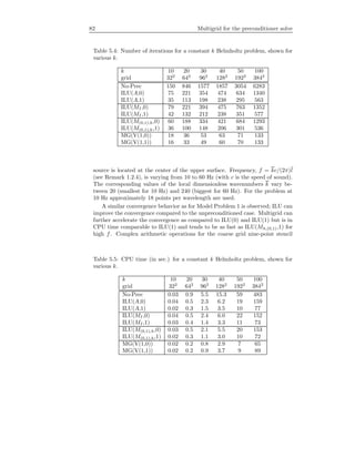
![5.5 Numerical results 83
elements may be the reason for the comparable CPU time of multigrid and
ILU(Mh,(0,1),1).
The use of a V-cycle with only a pre-smoothing step for the preconditioner is
the best option w.r.t. multigrid; The combination Bi-CGSTAB and ILU(1) for
Mh,(0,1) solves the problem fastest among the choices presented. For high fre-
quencies, the complex shifted-Laplace preconditioner Mh,(0,1) does not indicate
any breakdown of the iterations, whereas the SV preconditioner did (CPU time
is not available for SV in [81]). The performance of the complex shifted-Laplace
preconditioner behaves well; the number of iterations increases almost linearly
against f.
Table 5.6: Number of iterations for the wedge problem, shown for various fre-
quencies f.
f (Hz) 10 20 30 40 50
grid 76 × 126 151 × 251 232 × 386 301 × 501 376 × 626
No-Prec 2379 4057 6907 8248 >10000
ILU(A,0) 571 1339 1917 2443 3287
ILU(A,1) 239 563 832 1120 1418
ILU(MI ,0) 529 1066 1718 2173 2959
ILU(MI ,1) 235 531 787 903 1056
ILU(M(0,1),h,0) 485 997 1759 2082 2824
ILU(M(0,1),h,1) 212 426 664 859 1005
MG(V(1,0)) 48 92 132 182 213
MG(V(1,1)) 44 91 128 182 223
MSV 14 45 167 830 >2000
5.5.3 Model Problem 3: The Marmousi problem
The last example is Model Problem 3 (see Section 2.6): a part of the Marmousi
problem which mimics subsurface geology (see also Figure 2.4) with α = 0. The
domain is taken to be rectangular with a dimension of 6000 × 1600 m2
. The
Sommerfeld radiation condition is imposed at the boundary, and a point source
is placed at the center of the upper surface. The minimum number of points per
wavelength equals 17. The frequency is varied between 1 and 30 Hz. The number
of iterations and CPU time are presented in Tables 5.8 and 5.9, respectively, for
frequencies ranging from 1 to 30 Hz, with the termination criterion (5.30).
Whereas the iteration with ILU(0) hardly converges, not even for frequency
f = 1 Hz, the complex shifted-Laplace preconditioner accelerates the iteration
effectively. For low frequencies, the SV preconditioner outperforms the complex
shifted Laplace preconditioner, but the latter is faster as the frequency increases.
Even though multigrid can help reduce the number of iterations, it brings
only about 20% reduction in the CPU-time compared to ILU(1), see Table 5.9.](https://image.slidesharecdn.com/erlangga-160128071050/85/Erlangga-97-320.jpg)
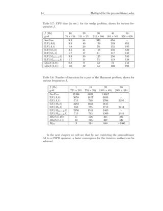
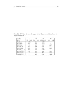

![Chapter 6
Multigrid-based
preconditioner for the
Helmholtz equation
In Chapter 4 we introduced a preconditioner for high wavenumber Helmholtz
problems in heterogeneous media. The preconditioner was based on the Laplace
operator with a zeroth-order imaginary term. In Chapter 5, in the context of
preconditioned Krylov subspace methods, we have advocated the use of multi-
grid to approximately invert the preconditioner. Numerical results suggested
that one multigrid iteration for the preconditioner solve is sufficient to result in
a fast converging Krylov subspace method. The choice of preconditioner was,
however, restricted by the fact that we only allowed the real part of the pre-
conditioning matrix to be (positive) definite. In this chapter we will be more
flexible in the choice of the parameters in the preconditioner. With more flexi-
bility, we will see that the preconditioned system leads to a favorably clustered
spectrum for a Krylov subspace convergence acceleration.
In this chapter we benefit from Fourier analysis in several ways. First of
all, for idealized (homogeneous boundary conditions, constant coefficients) ver-
sions of the preconditioned system it is possible to visualize its spectrum for
different values of the wavenumber, as Fourier analysis provides all eigenvalues,
Section 6.1. Secondly, for analyzing multigrid algorithms quantitatively Fourier
smoothing, two- and three-grid analysis [20, 21, 89, 92, 106] are the analysis
tools of choice.
In the end of this chapter, convergence results are shown for the set of 2D
model problems described in Section 2.6. These results shows that with more
flexibility in the choice of parameters β1 and β2 in the preconditioning operator,
a significant convergence improvement can be obtained.](https://image.slidesharecdn.com/erlangga-160128071050/85/Erlangga-101-320.jpg)
![88 Multigrid-based preconditioner for the Helmholtz equation
6.1 More on the spectral properties of the shifted
Laplace preconditioner
Our starting point is the shifted Laplace operator (4.14) written for 2D case as
M(β1,β2) := −∆ − (β1 − ˆjβ2)k2
, (6.1)
with (β1, β2) now any arbitrary real value. Boundary conditions are set identical
to those for the original Helmholtz problem. One member of the family is M(0,1),
which was analyzed thoroughly in the previous two chapters. In addition to this
choice, we include in this chapter some more values for (β1, β2).
We perform Fourier analysis to investigate the effect of the choice of (β1, β2)
in the preconditioner on the clustering of the eigenvalues of the preconditioned
system. For this we consider operator (5.13) with homogeneous Dirichlet bound-
ary conditions, wavenumber k constant, a discrete version of Helmholtz opera-
tor (1.26), Ah, and of preconditioner (6.1), Mh. For both Ah and Mh we choose
the 5-point stencil. The components (5.12) are eigenfunctions of these discrete
operators with constant coefficients. With these eigenfunctions AhM−1
h is di-
agonalizable and the eigenvalues are easily determined. In the first tests we
do not include damping in Ah, so α = 0 in (1.26). We consider several possi-
bilities: β = (β1, β2) = {(0, 0), (−1, 0), (0, 1), (1, 1), (1, 0.5), (1, 0.3)}. The first
three pairs are known: β = (0, 0) is from Bayliss [12], β = (−1, 0) from [64],
and β = (0, 1) as in [37, 38, 40] (see Chapters 4 and 5). The pairs with β1 = 1
are new here. So we reduce the imaginary term in such a way that the operator
M(β1,β2) approximates the Helmholtz operator A. Again, we use the notation
Mh,(β1,β2) to indicate the discrete version of M(β1,β2) (6.1).
Figure 6.1 presents the spectra of AhM−1
h for Mh,(0,0), Mh,(−1,0), Mh,(0,1),
Mh,(1,1), Mh,(1,0.5) and Mh,(1,0.3). The results are for k = 40 (k2
= 1600),
h = 1/64. Similar eigenvalue distributions are observed for finer grids.
From the spectra presented with the shifted Laplace preconditioner the lower
pictures of Figure 6.1 are favorable as their real parts vary between 0 and 1.
Preconditioner Mh,(0,0) in Figure 6.1a exhibits large isolated eigenvalues; for
Mh,(−1,0) the eigenvalues in Figure 6.1b are distributed between −1 and 1 on
the real axis. The preconditioners with complex Helmholtz terms give rise to
a curved spectrum. Whereas the real part of the spectrum in Figure 6.1c still
includes a part of the negative real axis, this is not the case for the (β1, β2)-
preconditioners with β1 = 1. The difference between Figures 6.1d, 6.1e and 6.1f
is that with a smaller value of β2 fewer outliers close to the origin are observed.
This is favorable for the convergence of the preconditioned Krylov methods.
The approximate inversion of the preconditioner itself by multigrid, however,
will be shown to be harder for smaller values of β2.
In Figure 6.2 the spectra for k = 100 (k2
= 104
) on a grid with h = 1/160
are presented for β1 = 1 and β2 varying between 1 and 0.3. The spectra are
very similar to those in Figure 6.1. More eigenvalues lie, however, in the vicinity
of the origin, due to the higher wavenumber and the correspondingly finer grid.](https://image.slidesharecdn.com/erlangga-160128071050/85/Erlangga-102-320.jpg)
![6.2 Multigrid for the preconditioner 89
(a) (b) (c)
0 0
0
11−1 0 0−0.20−80
(e)(d)
0
0
1 0 1
0
0 1
0
(f)
i i i
0.5i 0.5i 0.5i
−i −0.4i
−0.5i −0.5i−0.5i
−i
Figure 6.1: Spectral pictures of AhM−1
h with α = 0 and different values of
(β1, β2) in (6.1): (a) Mh,(0,0), (b) Mh,(−1,0), (c) Mh,(0,1), (d) Mh,(1,1), (e)
Mh,(1,0.5), (f) Mh,(1,0.3).
Figure 6.3 then presents the distribution of eigenvalues for the case that 5%s
damping (α = 0.05) is set in A. Parameters in the preconditioner are (β, β2) =
(1, 0.5). Again the 5-point stencil is used for discretization. Figure 6.3a presents
the spectrum for k = 40, h = 1/64, and Figure 6.3b for k = 100, h = 1/160. An
interesting observation is that now the eigenvalues move away from the origin
into the right half plane. This is beneficial for iterative solution methods. From
the spectra in Figure 6.3 it is expected that the Bi-CGSTAB convergence in the
case of damping will be considerably faster than for the undamped case. As
the circles have moved away from the origin it is possible to apply the classical
theory of the GMRES convergence [84, 83], for example. One can place an
ellipse around the spectrum. As it becomes a circle in the case of damping, it is
expected that the resulting bounds for the GMRES convergence will be sharp.
6.2 Multigrid for the preconditioner
6.2.1 Fourier analysis and multigrid results
We first consider here solely the preconditioner M(β1,β2) (6.1) and compare the
numerical multigrid convergence with asymptotic convergence factors µ, ρ2g, ρ3g
from Fourier analysis. (The behavior of the complete solution method will be
considered in the next section.) Wavenumber k is taken constant here and a
square domain with an equidistant grid is used. The second order Sommerfeld](https://image.slidesharecdn.com/erlangga-160128071050/85/Erlangga-103-320.jpg)
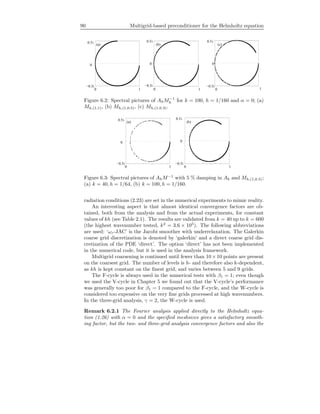
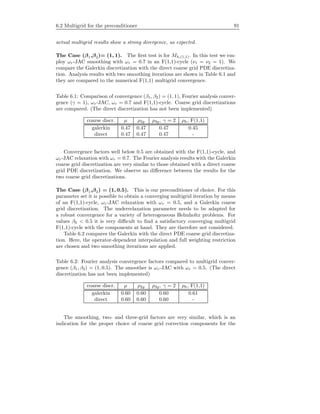
![92 Multigrid-based preconditioner for the Helmholtz equation
problems under investigation. The numerical convergence with the F(1,1)-cycle
is again very similar to the Fourier results.
In the following three remarks we explain the satisfactorily convergence with
standard multigrid for the complex Helmholtz equation and β1 = 1 with some
heuristic arguments.
Remark 6.2.2 Smoothing. The Fourier symbol of ωr-JAC for the complex
Helmholtz equation reads
Sh = 1 −
ωr
4 − (β1 − β2
ˆj)(hk)2
4 − (β1 − β2
ˆj)(hk)2
− 2 cos 1πh − 2 cos 2πh ,
1, 2 = 1, . . . ,
√
N − 1.
We consider the case k = 40, h = 1/64 and take ωr as in the previous ex-
periments. Table 6.3 presents smoothing factors on four consecutive grids for
(β1, β2) = (1, 0) (original Helmholtz equation) and for (β1, β2) = (0, 1), (1, 1)
and (1, 0.5). For simplicity, a direct PDE discretization on the coarse grids has
been used.
Table 6.3: Smoothing factors µh for ωr-JAC on different coarse grids and various
(β1, β2)-values.
(β1, β2) ωr in ωr-JAC h :
1/64 1/32 1/16 1/8
(1, 0) 0.7 0.47 0.75 2.31 0.18
(0, 1) 0.8 0.36 0.32 0.13 0.05
(1, 1) 0.7 0.47 0.56 0.35 0.13
(1, 0.5) 0.5 0.60 0.77 0.81 0.32
From Table 6.3, one finds that for h = 1/16 ωr-JAC diverges for the orig-
inal Helmholtz operator (also found with other relaxation parameters). This
is in accordance with the remarks in [23, 33], that smoothing problems do not
occur on the very fine or the very coarse grids, but on the intermediate grids.
Furthermore, it can be observed that the (β1, β2) = (0, 1)-preconditioner re-
sembles a Laplace-type situation, with excellent smoothing factors on all grids.
The preconditioners with β1 = 1 give smoothing factors less than one on every
grid. The (1, 1)-preconditioner exhibits better smoothing factors than the set
(β1, β2) = (1, 0.5), which represents a limit case for which smoothing factors are
still below one.
Remark 6.2.3 Simplified coarse grid analysis. Some insight into the coarse
grid correction can be gained from the so-called ‘simplified coarse grid analysis’
or first-differential-approximation analysis [21, 23, 92]. As in [33] we apply
this analysis for a 1D Helmholtz operator. Assuming that transfer operators
do not have any effect on the lowest frequencies, the quantity 1 − λ 1
h /λ2 1
2h ( 1](https://image.slidesharecdn.com/erlangga-160128071050/85/Erlangga-106-320.jpg)
![6.2 Multigrid for the preconditioner 93
small) gives some insight into the relation between the discrete fine and coarse
grid operators. This quantity should be close to zero and is an indication of the
suitability of a coarse grid operator in multigrid. For the original 1D Helmholtz
equation and α = 0 (no damping) this quantity reads [33]:
1 − λ 1
h /λ2 1
2h =
sin4
( 1hπ/2)
sin2
( 1hπ/2) cos2 ( 1hπ/2) − (kh/2)2
, 1 = 1, . . . , N.
It may give rise to a problematic coarse grid correction in the range where
sin2
( 1hπ/2) cos2
( 1hπ/2) ≈ (kh/2)2
and 1 is associated with a smooth mode. For a 1D version of the complex
Helmholtz operator, this quantity reads
1 − λ 1
h /λ2 1
2h =
sin4
( 1hπ/2)
sin2
( 1hπ/2) cos2 ( 1hπ/2) − (kh/2)2(β1 − β2
ˆj)
=
sin4
( 1hπ/2) sin2
( 1hπ/2) cos2
( 1hπ/2) − (kh/2)2
(β1 + β2
ˆj)
sin2
( 1hπ/2) cos2 ( 1hπ/2) − (kh/2)2β1
2
+ (kh/2)2β2
2
,
1 = 1, . . . , N.
This expression for the complex Helmholtz operator is close to zero for the
(β1, β2)-sets under consideration: the denominator does not reach zero, and the
numerator contains the term sin4
hπ/2 which is very small for smooth eigen-
modes.
Remark 6.2.4 h-ellipticity. When a Galerkin coarse grid discretization is
used, it is difficult to gain insight into the coarse grid correction, as the coarse
grid stencil elements are constructed with nontrivial formulas. Therefore, we
discuss here for the case (β1, β2) = (1, 0.5) two coarse grid discretizations. With
h = 1/64, k = 40, α = 0 in the five-point stencil, we obtain by direct PDE
discretization similar coarse grid stencils as the fine grid stencil with grid sizes
2h or 4h, respectively. In that case, only the central stencil element contains an
imaginary contribution. When the Galerkin coarse grid operator is employed,
the imaginary part is distributed over all entries. With operator-dependent in-
terpolation and full weighting restriction we find,
A2h
∧
=
−282.9 + 15.3ˆj −665.8 + 80.6ˆj −282.9 + 15.3ˆj
−665.8 + 80.6ˆj 2164.5 + 461.2ˆj −665.8 + 80.6ˆj
−282.9 + 15.3ˆj −665.8 + 80.6ˆj −282.9 + 15.3ˆj
,
A4h
∧
=
−129.5 + 43.0ˆj −290.1 + 135.0ˆj −129.5 + 43.0ˆj
−290.1 + 135.0ˆj −101.4 + 483.2ˆj −290.1 + 135.0ˆj
−129.5 + 43.0ˆj −290.1 + 135.0ˆj −129.5 + 43.0ˆj
.(6.2)
The h-ellipticity measures, indicating the suitability of the stencils for point-
wise smoothing [21, 92], are 0.28 and 0.18. For the direct PDE discretization](https://image.slidesharecdn.com/erlangga-160128071050/85/Erlangga-107-320.jpg)
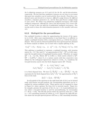
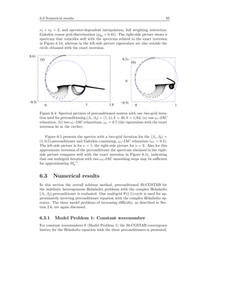
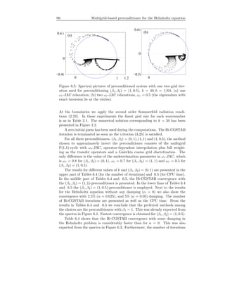
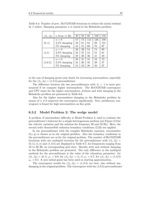
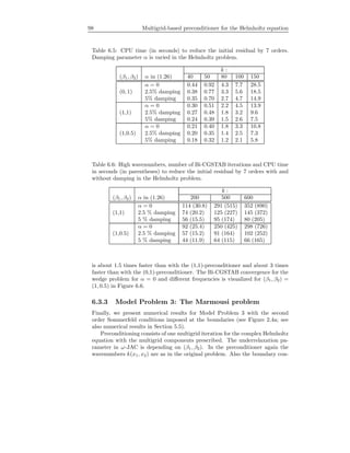
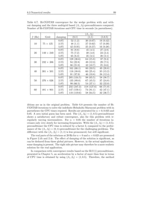
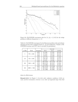
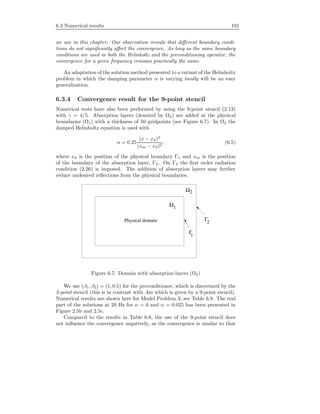
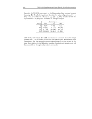
![Chapter 7
Three-dimensional
Helmholtz equation
In the preceding chapters we have show that multigrid applied to the shifted
Laplace preconditioner can effectively enhance the convergence of Krylov sub-
space methods (which, in this case, is Bi-CGSTAB) for the 2D heterogeneous
Helmholtz equation at high wavenumbers. It has been shown, theoretically and
numerically, that the convergence is h-independent and mildly depends on the
wavenumber k for the undamped case (α = 0). For Helmholtz problems with
damping (α ∼ 0.05) the convergence is observed to be also independent of k.
In this chapter we discuss the extension of the method to 3D [39]. The gen-
eral algorithm is similar: multigrid-based preconditioners within Bi-CGSTAB.
For Bi-CGSTAB the algorithm is immediately extendable to 3D. For multigrid,
however, a multigrid algorithm with semicoarsening is employed. By this the
coarsening is not done in all three directions. Rather, one does coarsening in
one or two directions, while the other directions are uncoarsened, in which line
(or plane) smoothing is applied. After introducing the 3D Helmholtz equation
and the 3D preconditioner, a multigrid method with semicoarsening for approx-
imately inverting the preconditioner is discussed in Section 7.2. Applications of
the method to 3D model problems are given in Section 7.3.
7.1 3D Helmholtz equation
We consider the three-dimensional Helmholtz equation in a 3D rectangular do-
main Ω ⊂ R3
:
Au := − ∂x1x1 + ∂x2x2 + ∂x3x3 + (1 − αˆj)k2
u = g, (7.1)
with boundary conditions on Γ ≡ ∂Ω as determined by (2.23)–(2.26). Equation
(7.1) is discretized using the standard 7-point finite difference stencil.](https://image.slidesharecdn.com/erlangga-160128071050/85/Erlangga-117-320.jpg)
![104 Three-dimensional Helmholtz equation
In 3D the preconditioning operator reads
M := − ∂x1x1 + ∂x2x2 + ∂x3x3 + (1 − 0.5ˆj)k2
. (7.2)
In this chapter we simplify the notation for the shifted Laplace preconditioner as
we only consider one particular case with (β1, β2) = (1, 0.5). So, here M always
refers to M(1,0.5). The preconditioner M is then constructed from discretiza-
tion of (7.2) using the 7-point finite difference stencil, with the same boundary
conditions as for (7.1). The right preconditioned linear system to solve is then
given as
AhM−1
h wh = gh, wh = Mhuh, (7.3)
where Mhuh = wh is to be solved approximately using one multigrid iteration.
7.2 Multigrid with semicoarsening for the pre-
conditioner
For a three-dimensional problem, the choice of multigrid components is richer
than in two dimensions. For the 3D Poisson equation, multigrid method with
standard coarsening and point-wise smoothing already results in a good con-
vergence. For anisotropic Poisson problems, however, multigrid with standard
coarsening and point smoother is not sufficient; the convergence rate is not the
typically fast multigrid convergence. For such problems, the use of line (or
plane) smoothers is important. A point smoother can only produce fast multi-
grid convergence if a semicoarsening strategy is incorporated (see [91]). For
more complicated situations, where strong variations exist in an arbitrary way
in the domain, the use of algebraic multigrid is a natural choice (not treated in
this thesis).
The shifted Laplace operator does not seem to require a non-standard multi-
grid method; multigrid method with point smoother seems sufficient. This is an
observation in 2D, even for Helmholtz problems with strong heterogeneities (see
Chapter 6). We, however, prefer to use a multigrid method with semicoarsening
because if coarsening is only done in two directions, all 2D multigrid compo-
nents (which were analyzed in Chapters 5 and 6) can be immediately used in
a 3D setting. For example, the interpolation operator can be built based on
bilinear interpolation or operator-dependent interpolation by de Zeeuw. The
restriction operator can also be determined in the same way as in 2D. In the
third direction, where the grid is kept uncoarsened, line smoothing is employed.
Furthermore, a 2D parallelization strategy can immediately be adopted in 3D.
A discussion on multigrid with semicoarsening can be found, e.g. in [73, 78],
for multiple semicoarsened grids (MSG) method, or in [77] for the so-called
MG-S method, which is also based on multiple semicoarsening. For MG-S, the
behavior of the method can be analyzed based on standard multigrid methods.
Processing the semicoarsened grids in the case of MG-S can be viewed as a](https://image.slidesharecdn.com/erlangga-160128071050/85/Erlangga-118-320.jpg)
![7.2 Multigrid with semicoarsening for the preconditioner 105
smoothing iteration in the standard multigrid sequence. Extension of flexible
MG-S to 3D problems with anisotropy is presented in [104].
The 3D multigrid with (x1, x2) semicoarsening is illustrated in Figure 7.1
for three grid levels. In this case standard coarsening, i.e. doubling the mesh
size, only takes place in x1- and x2-directions, while the x3-direction is kept
uncoarsened. For the shifted Laplace operator (and the Helmholtz operator)
anisotropies do not appear. Therefore, the choice of coarsening is rather ar-
bitrary. We show in the numerical results in Section 7.3 that the choice of
coarsening direction does not have a significant effect to the convergence of the
method.
x
y
z
3,3,3
2,2,3
1,1,3
Figure 7.1: Semicoarsening of three grid levels: standard coarsening in two
directions (x1 and x2), the third (x3) direction is kept uncoarsened
Consider the preconditioning operator (7.2) which is discretized by the 7-
point stencil on a grid Gh = {(i1h, i2h, i3h)|i1, i2, i3 = 1, . . . , 3
√
N − 1}, with
h = 1/ 3
√
N. For a damped x3-line Jacobi relaxation with relaxation factor
0 < ωr ≤ 1 we have the following iteration:
(Mh,x3 + Dh)uj+1
h + (Mh,x1 + Mh,x2 )uj
h = wh, (7.4)
uj+1
h = ωruj+1
h + (1 − ωr)uj
h, (7.5)
with
(Mh,x1 u)i1,i2,i3 := −
1
h2
(ui1+1,i2,i3 + ui1−1,i2,i3 ) , (7.6)
(Mh,x2 u)i1,i2,i3 := −
1
h2
(ui1,i2+1,i3 + ui1,i2−1,i3 ) , (7.7)
(Mh,x3 u)i1,i2,i3 := −
1
h2
(ui1,i2,i3+1 + ui1,i2,i3−1) , (7.8)
(Dhu)i1,i2,i3 :=
1
h2
6 − (1 − 0.5ˆj)k2
h2
ui1,i2,i3 . (7.9)](https://image.slidesharecdn.com/erlangga-160128071050/85/Erlangga-119-320.jpg)
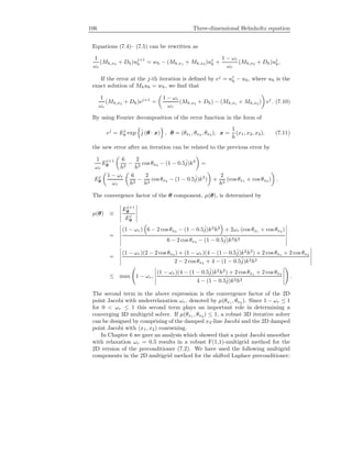
![7.2 Multigrid with semicoarsening for the preconditioner 107
• Restriction, IH
h : Gh → GH , is full weighting,
• Prolongation, Ih
H : GH → Gh, is bilinear interpolation or de Zeeuw’s
operator-dependent interpolation [109], and
• Galerkin coarse grid discretization AH = IH
h AhIh
H .
In the 3D multigrid method with semicoarsening, the same multigrid compo-
nents as in 2D are used. However, a slight adaptation is needed before one
realizes the same 2D interpolation and restriction operators in 3D semicoarsen-
ing.
Prolongation operator. To determine the 3D interpolation weights, we con-
sider the 27-point stencil matrix (see Figure 7.2), written as follows:
(Mu)i1,i2,i3
=
iz=−1,0,1
(m(iz)1
i1,i2,i3
ui1−1,i2−1,i3+iz +m(iz)2
i1,i2,i3
ui1,i2−1,i3+iz
+m(iz)3
i1,i2,i3
ui1+1,i2−1,i3+iz +m(iz)4
i1,i2,i3
ui1−1,i2,i3+iz
+m(iz)5
i1,i2,i3
ui1,i2,i3+iz +m(iz)6
i1,i2,i3
ui1+1,i2,i3+iz
+m(iz)7
i1,i2,i3
ui1−1,i2+1,i3+iz +m(iz)8
i1,i2,i3
ui1,i2+1,i3+iz
+m(iz)9
i1,i2,i3
ui1+1,i2+1,i3+iz).
(7.12)
1 2 3
4 5 6
7 8 9
iz = −1
iz = 0
iz = 1
x
z
y
Figure 7.2: The 27-point stencil](https://image.slidesharecdn.com/erlangga-160128071050/85/Erlangga-121-320.jpg)
![108 Three-dimensional Helmholtz equation
In case the coarsening is only done in (x1, x2) direction, a lumped 9-point
stencil matrix Mh in an (x1, x2)-plane is defined as:
(Mφ)i1,i2,i3 = m1
i1,i2,i3
ui1−1,i2−1,i3 + m2
i1,i2,i3
ui1,i2−1,i3 + m3
i1,i2,i3
ui1+1,i2−1,i3
+ m4
i1,i2,i3
ui1−1,i2,i3 + m5
i1,i2,i3
ui1,i2,i3 + m6
i1,i2,i3
ui1+1,i2,i3
+ m7
i1,i2,i3
ui1−1,i2+1,i3 + m8
i1,i2,i3
ui1,i2+1,i3 + m9
i1,i2,i3
ui1+1,i2+1,i3 ,
with
mp
i1,i2,i3
= m(−1)p
i1,i2,i3
+ m(0)p
i1,i2,i3
+ m(1)p
i1,i2,i3
, p = 1, 2, . . . , 9.
Based on the lumped 9-point stencil the coarse-to-fine grid interpolation can be
determined in the same way as described in Chapter 5 for bilinear interpolation
(BI) or in [109] for operator-dependent interpolation (MD).
Restriction operator. For the restriction operator we use the full weight-
ing (5.22) instead of the adjoint of the interpolation operator. In the (x1, x2)
semicoarsening setting the implementation of the 2D full weighting operator is
straightforward.
7.3 Numerical results
In this section we present numerical results from several 3D model problems, as
depicted in Figure 7.3 and 7.4. Since the numerical experiments are performed
on a single processor machine, the problem size that can be resolved is limited. A
parallel implementation in 3D becomes inevitable. The examples here, however,
are representative to show that the shifted Laplace preconditioner is robust and
effective to accelerate the Krylov subspace methods applied to the Helmholtz
equation in general dimensions with regular heterogeneities. There is no reason
to believe that the solver will not perform well for irregular heterogeneities.
7.3.1 3D constant wavenumber
We first consider a problem at constant wavenumber and α = 0 (undamped)
in Ω = (0, 1)3
. At the boundaries Γ = ∂Ω the first-order radiation conditions
are prescribed, that are discretized by a one-sided finite difference scheme. A
unit source is situated at x = (1
2 , 1
2 , 1
2 ). Starting with a zero initial guess,
Bi-CGSTAB runs until the residual is reduced by 7 orders of magnitude, as
in (3.25).
The numerical performance is shown in Table 7.1 for various wavenumbers
k, obtained on grids of resolution kh = 0.625 (∼ 10 grid points per wavelength).
Compared to Model Problem 1 in 2D, the 3D convergence results show a similar
performance as their 2D counterparts, or even faster convergence is observed.
In the constant wavenumber case, the use of bilinear or operator-dependent in-
terpolation in multigrid does not lead to a different computational performance.](https://image.slidesharecdn.com/erlangga-160128071050/85/Erlangga-122-320.jpg)
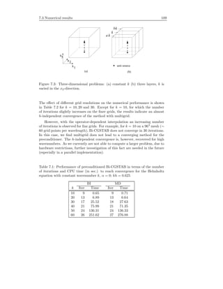
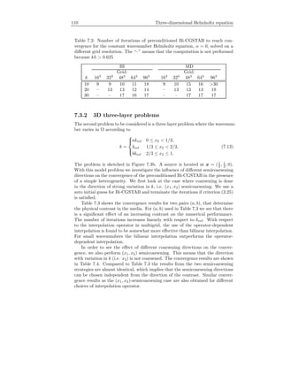
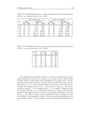
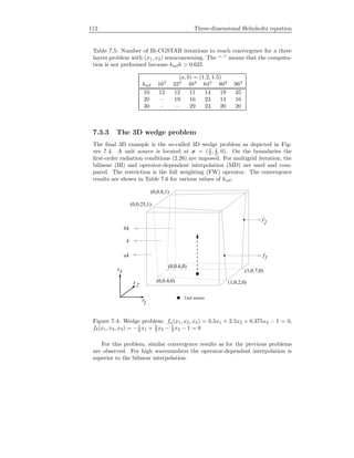
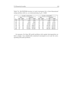

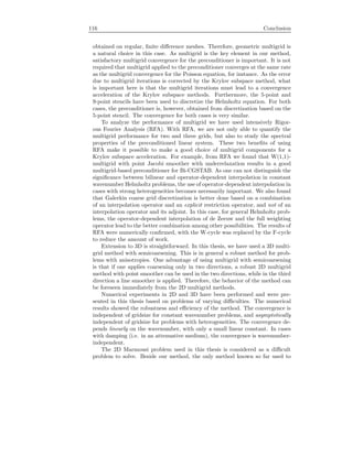
![8.2 Remark 117
iteratively solve this problem is Bi-CGSTAB with the separation-of-variables
preconditioner [81]. This method, however, does not converge after 2000 itera-
tions at f = 30 Hz. To our knowledge, our method is the first iterative method
which is able to reach convergence for the Marmousi problem with satisfactory
performance (for f = 30 Hz, 136 iterations).
8.2 Remark
Deflation
From the spectral analysis of the preconditioned system we observed that many
eigenvalues lie very close to zero in the complex plane. This bunch of small eigen-
values is responsible for slow convergence in the first few iterations of Krylov
subspace iterations, before the fast convergence is obtained. This is called su-
perlinear convergence, and observed in our numerical tests.
In [76, 24, 43] so-called deflation is used to project out the smallest eigenval-
ues from the original spectrum. As their components no longer contribute to the
residual (or error), the convergence rate improves. In deflation a deflation sub-
space must be constructed, which is usually based on eigenvectors corresponding
to the removed eigenvalues. For a small number of small eigenvalues, say ∼ 5,
corresponding to a small matrix A, the projection matrix can be easily deter-
mined. A problem arises when a bunch of too many small eigenvalues has to be
projected out from the spectrum. Computing the corresponding eigenvectors is
then too expensive.
As advocated in [43, 103] the projection matrix can be approximately con-
structed based on spectral properties of the problem. Thus, one needs not define
the projection matrix exactly. For our case, if a similar approach can also be
realized, a faster convergence of the method can be expected.
Finite element implementation
Many applications of the Helmholtz equation involve complicated geometries.
For such geometries a finite element discretization is a natural choice. In this
thesis we did not treat finite element methods. The method, however, is easily
extended to finite elements. For finite element matrices, algebraic multigrid is
then the natural choice.
Parallel implementation
In geophysical applications, one usually encounters huge problems that lead to
huge matrices. In 3D, for instance, the number of unknowns to be resolved is of
order of billions, which is too huge to be fitted in one computer. For a realistic
3D problem, and to some extent for 2D, parallel implementation of the method
becomes inevitable.
The method proposed in this thesis is fully parallelizable. Every step in the
Bi-CGSTAB algorithm is parallelizable: the matrix-vector multiplications, the](https://image.slidesharecdn.com/erlangga-160128071050/85/Erlangga-131-320.jpg)
![118 Conclusion
inner products and preconditioner solves. For the latter we have chosen multi-
grid components such that the multigrid algorithm can be fully implemented
in a parallel machine. The Jacobi smoother, for example, not only turns out
to be an efficient smoother for the shifted Laplace operator, but it is also fully
parallelizable.
Currently, a parallel implementation is carried out and preliminary results
from 2D tests indicate a good scalability of the method.
Seismic application: migration
As stated in Chapter 1, the target application of the method is in 2D/3D
frequency-domain migration in seismics. This is done by resolving the Helmholtz
equation for a range of frequencies and recording the solution of each frequency
on some locations of the receiver on the earth’s surface. Once all of these so-
lutions are obtained, time domain solution can be recovered by Fast-Fourier
transforming the frequency-domain solutions.
We currently carry out a migration computation for a synthetic model based
on the full Marmousi problem, and the results will be part of our publication
in [36].](https://image.slidesharecdn.com/erlangga-160128071050/85/Erlangga-132-320.jpg)
![Bibliography
[1] S. Abarbanel and D. Gottlieb, A mathematical analysis of the PML
method, J. Comput. Phys., 134 (1997), pp. 357–363.
[2] , On the construction and analysis of absorbing layers in CEM, Appl.
Numer. Math., 27 (1998), pp. 331–340.
[3] R. E. Alcouffe, A. Brandt, J. E. Dendy Jr, and J. W. Painter,
The multi-grid method for the diffusion equation with strongly discontin-
uous coefficients, SIAM J. Sci. Comput., 2 (1981), pp. 430–454.
[4] A. Arnold and M. Ehrhardt, Discrete transparent boundary condi-
tions for wide angle parabolic equations in underwater acoustics, J. Com-
put. Phys., 145 (1998), pp. 611–638.
[5] O. Axelsson, A survey of preconditioned iterative methods for linear
systems of algebraic equations, BIT, 25 (1985), pp. 166–187.
[6] O. Axelsson and G. Lindskog, On the rate of convergence of the pre-
conditioned conjugate gradient method, Numer. Math., 48 (1986), pp. 499–
523.
[7] I. Babuska, F. Ihlenburg, T. Strouboulis, and S. K. Gangaraj,
Posteriori error estimation for finite element solutions of Helmholtz’s
equation. Part I: The quality of local indicators and estimators, Int. J.
Numer. Methods. Engrg., 40 (1997), pp. 3443–3462.
[8] , Posteriori error estimation for finite element solutions of
Helmholtz’s equation. Part II: Estimation of the pollution error, Int. J.
Numer. Methods. Engrg., 40 (1997), pp. 3883–3900.
[9] I. Babuska and S. Sauter, Is the pollution effect of the FEM avoidable
for the Helmholtz Equation considering high wave numbers?, SIAM J.
Numer. Anal., 27 (1997), pp. 323–352.
[10] A. Bamberger, B. Enquist, L. Halpern, and P. Joly, Parabolic
wave equation approximation in heterogeneous media, SIAM J. Appl.
Math., 48 (1988), pp. 99–128.](https://image.slidesharecdn.com/erlangga-160128071050/85/Erlangga-133-320.jpg)
![120 BIBLIOGRAPHY
[11] A. Bamberger, P. Joly, and J. E. Roberts, Second-order absorb-
ing boundary conditions for the wave equation: A solution for the corner
problem, SIAM J. Numer. Anal., 27 (1990), pp. 323–352.
[12] A. Bayliss, C. I. Goldstein, and E. Turkel, An iterative method for
Helmholtz equation, J. Comput. Phys., 49 (1983), pp. 443–457.
[13] , On accuracy conditions for the numerical computation of waves, J.
Comput. Phys., 59 (1985), pp. 396–404.
[14] J. P. Berenger, A perfectly matched layer for the absorption of electro-
magnetic waves, J. Comput. Phys., 114 (1994), pp. 185–200.
[15] , Three-dimensional perfectly matched layer for the absorption of
electromagnetic waves, J. Comput. Phys., 127 (1996), pp. 363–379.
[16] A. J. Berkhout, Seismic Migration: Imaging of Acoustic Energy by
Wave Field Extrapolation, Elsevier, Amsterdam, 1982.
[17] B. Biondi and G. Palacharla, 3-d prestack migration of common-
azimuth data, Geophysics, 61 (1996), pp. 1822–1832.
[18] A. Bourgeois, M. Bourget, P. Lailly, M. Poulet, P. Ricarte,
and R. Versteeg, Marmousi, model and data, in Marmousi Experience,
1991, pp. 5–16.
[19] K. Brackenridge, Multigrid and cyclic reduction applied to the
Helmholtz equation, in Proc. 6th Copper Mountain Conf. on Multigrid
Methods, N. D. Melson, T. A. Manteuffel, and S. F. McCormick, eds.,
1993, pp. 31–41.
[20] A. Brandt, Multi–level adaptive solutions to boundary–value problems,
Math. Comp., 31 (1977), pp. 333–390.
[21] , Multigrid techniques: 1984 guide with applications to fluid dynam-
ics, Tech. Rep. GMD-Studie 85, GMD Sankt Augustine, Germany, 2002.
[22] A. Brandt and I. Livshits, Wave-ray multigrid methods for standing
wave equations, Electr. Trans. Num. Anal., 6 (1997), pp. 162–181.
[23] A. Brandt and S. Ta’asan, Multigrid method for nearly singular and
slightly indefinite problems, in Proc. EMG’85 Cologne, 1986, pp. 99–121.
[24] A. Chapman and Y. Saad, Deflated and augmented krylov subspace
techniques, Numer. Linear Algebra Appl., 4(1) (1997), pp. 43–66.
[25] J. F. Claerbout, Imaging the Earth’s Interior, Blackwell Scientific Pub-
lications, 1985.
[26] R. Clayton and B. Engquist, Absorbing boundary conditions for
acoustic and elastic wave equations, Bull. Seis. Soc. America, 67(6) (1977),
pp. 1529–1540.](https://image.slidesharecdn.com/erlangga-160128071050/85/Erlangga-134-320.jpg)
![BIBLIOGRAPHY 121
[27] , Absorbing boundary conditions for wave-equation migration, Geo-
physics, 45(5) (1980), pp. 895–904.
[28] F. Collino and P. Joly, Splitting of operators, alternate directions, and
paraxial approximations for the three-dimensional wave equation, SIAM J.
Sci. Comput., 16 (1995), pp. 1019–1048.
[29] D. Colton and R. Kress, Inverse matrix and electromagnetic scattering
theory, Springer Verlag, Berlin-Heidelberg, 1998.
[30] J. Dendy, Jr., Blackbox multigrid for nonsymmetric problems, Appl.
Math. Comput., 13 (1983), pp. 261–283.
[31] A. Deraemaeker, I. Babuska, and P. Bouillard, Dispersion and
pollution of the FEM solution for the Helmholtz equation in one, two, and
three Dimensions, Int. J. Numer. Methods Engrg., 46 (1999), pp. 471–499.
[32] J. Douglas, J. Hensley, and J. E. Roberts, An alternating-direction
iteration method for Helmholtz problems, Appl. Math., 38 (1993), pp. 289–
300.
[33] H. R. Elman, O. G. Ernst, and D. P. O’Leary, A multigrid method
enhanced by Krylov subspace iteration for discrete helmholtz equations,
SIAM J. Sci. Comput., 31 (2001), pp. 1291–1315.
[34] B. Engquist and A. Majda, Absorbing boundary conditions for the
numerical simulation of waves, Math. Comput., 31 (1977), pp. 629–651.
[35] Y. A. Erlangga, C. W. Oosterlee, and C. Vuik, A novel multigrid-
based preconditioner for the heterogeneous helmholtz equation, SIAM J.
Sci. Comput., (to appear).
[36] Y. A. Erlangga, R. E. Plessix, W. A. Mulder, C. vuik, and
C. W. Oosterlee, A new iterative solver for the time-harmonic wave
equation applied to seismic problems, Geophysics, submitted (2005).
[37] Y. A. Erlangga, C. Vuik, and C. W. Oosterlee, On a class of pre-
conditioners for solving the the discrete helmholtz equation, in Mathemat-
ical and Numerical Aspects of Wave Propagation, G. Cohen, E. Heikkola,
P. Joly, and P. Neittaanm akki, eds., Univ. Jyv¨askyl¨a, Finland, 2003,
pp. 788–793.
[38] , On a class of preconditioners for solving the Helmholtz equation,
Appl. Numer. Math., 50 (2004), pp. 409–425.
[39] , Krylov subspace iterative methods accelerated with multigrid for
the 3d heterogeneous helmholtz equation, in Mathematical and Numeri-
cal Aspects of Wave Propagation, Brown University, Rhode Island, 2005,
pp. 418–419.](https://image.slidesharecdn.com/erlangga-160128071050/85/Erlangga-135-320.jpg)
![122 BIBLIOGRAPHY
[40] , Comparison of multigrid and incomplete LU shifted-Laplace precon-
ditioners for the inhomogeneous Helmholtz equation, Appl. Numer. Math.,
(in press).
[41] G. J. Fix and S. P. Marin, Variational methods for underwater acoustic
problems, J. Comput. Phys., 28 (1978), pp. 253–270.
[42] R. Fletcher, Conjugate gradient methods for indefinite systems, in Proc.
the 1974 Dundee Biennial Conf. on Numerical Analysis, G. A. Watson,
ed., 1975, pp. 73–89.
[43] J. Frank and C. Vuik, On the construction of the deflated-based pre-
conditioner, SIAM J. Sci. Comput., 23(2) (2001), pp. 442–462.
[44] R. W. Freund, Conjugate gradient-type methods for linear systems with
complex symmetric coefficient matrices, SIAM J. Sci. Stat. Comput., 13(1)
(1992), pp. 425–448.
[45] , Preconditioning of symmetric but highly indefinite linear systems,
in 15th IMACS World Congress on Scientific Computation Modelling and
Applied Mathematics, Vol. 2 Numerical Mathematics, A. Sydow, ed.,
1997, pp. 551–556.
[46] R. W. Freund and N. M. Nachtigal, QMR: A quasi minimum resid-
ual method for non-Hermitian linear systems, Numer. Math., 60 (1991),
pp. 315–339.
[47] M. J. Gander and F. Nataf, AILU for Helmholtz problems: A new
preconditioner based on the analytic parabolic factorization, J. Comput.
Acoustics, 9 (2001), pp. 1499–1509.
[48] A. George and J. W. Liu, Computer solution of large sparse positive
definite systems, Prentice-Hall Inc., NJ, 1981.
[49] D. N. Ghosh-Roy and L. S. Couchman, Inverse problems and inverse
scattering of plane waves, Academic Press, London, 2002.
[50] D. Givoli and I. Patlashenko, Optimal local non-reflecting boundary
conditions, Appl. Numer. Math., 27 (1998), pp. 367–384.
[51] J. Gozani, A. Nachshon, and E. Turkel, Conjugate gradient coupled
with multigrid for an indefinite problem, in Advances in Comput. Methods
for PDEs V, 1984, pp. 425–427.
[52] M. H. Gutknecht, Variants of BICGSTAB for matrices with complex
spectrum, SIAM J. Sci. Comput., 14(5) (1993), pp. 1022–1033.
[53] W. Hackbusch, Multi-Grid Methods and Applications, Springer-Verlag,
Berlin, 2003.](https://image.slidesharecdn.com/erlangga-160128071050/85/Erlangga-136-320.jpg)
![BIBLIOGRAPHY 123
[54] I. Harari and E. Turkel, Accurate finite difference methods for time-
harmonic wave propagation, J. Comput. Phys., 119 (1995), pp. 252–270.
[55] E. Heikkola, T. Rossi, and J. Toivanen, A parallel fictitious domain
decomposition method for the three-dimensional Helmholtz equation, tech.
rep., Dept. Math. Info. Tech., Univ. J¨yvask¨yla, No. B 9/2000, 2000.
[56] R. L. Higdon, Numerical absorbing boundary conditions for the wave
equation, Math. Comp., 49(179) (1987), pp. 65–90.
[57] F. Ihlenburg and I. Babuska, Dispersion analysis and error estima-
tion of Galerkin finite element methods for the Helmholtz equation, Int. J.
Numer. Methods Engrg., 38 (1995), pp. 3745–3774.
[58] , Finite element solution of the Helmholtz equation with high wave
number. Part I: The h-version of the FEM, Comput. Math. Appl., 30(9)
(1995), pp. 9–37.
[59] , Finite element solution of the Helmholtz equation with high wave
number. Part II: The hp-version of the FEM, SIAM J. Numer. Anal., 34
(1997), pp. 315–358.
[60] S. W. Jin and G. Peng, Prestack depth migration using a hybrid pseudo-
screen propagator, in 68th SEG Annual Mtg., 1998, pp. 1819–1822.
[61] C.-H. Jo, C. Shin, and J. H. Suh, An optimal 9-point, finite difference,
frequency space, 2-D scalar wave extrapolator, Geophysics, 61(2) (1996),
pp. 529–537.
[62] R. Kettler, Analysis and comparison of relaxation schemes in robust
multigrid and preconditioned conjugate gradient methods, in Multigrid
methods. Lecture Notes in Mathematics 960, W. Hackbusch and U. Trot-
tenberg, eds., 1982, pp. 502–534.
[63] S. Kim and S. Kim, Multigrid simulation for high-frequency solutions of
the Helmholtz problem in heterogeneous media, SIAM J. Sci. Comput., 24
(2002), pp. 684–701.
[64] A. L. Laird and M. B. Giles, Preconditioned iterative solution of the
2D Helmholtz equation, Tech. Rep. NA 02-12, Comp. Lab., Oxford Univ.,
2002.
[65] B. Lee, T. A. Manteuffel, S. F. McCormick, and J. Ruge, First-
order system least-squares for the Helmholtz equation, SIAM J. Sci. Com-
put., 21 (2000), pp. 1927–1949.
[66] S. K. Lele, Compact finite difference schemes with spectral-like resolu-
tion, J. Comput. Phys., 103(1) (1992), pp. 16–42.
[67] E. L. Lindman, Free space boundary conditions for time dependent wave
equation, J. Comput. Phys., 18 (1975), pp. 66–78.](https://image.slidesharecdn.com/erlangga-160128071050/85/Erlangga-137-320.jpg)
![124 BIBLIOGRAPHY
[68] R. E. Lynch and J. R. Rice, A high-order difference method for differ-
ential equations, Math. Comp., 34(150) (1980), pp. 333–372.
[69] M. M. M. Made, Incomplete factorization-based preconditionings for
solving the Helmholtz equation, Int. J. Numer. Meth. Engng., 50 (2001),
pp. 1077–1101.
[70] A. Majda and S. Osher, Reflection of singularities at the boundary,
Comm. Pure Appl. Math., 28 (1975), pp. 277–298.
[71] T. A. Manteuffel and S. V. Parter, Preconditioning and boundary
conditions, SIAM J. Numer. Anal., 27(3) (1990), pp. 656–694.
[72] K. J. Marfurt, Accuracy of finite-difference and finite-element modeling
of the scalar and elastic wave equations, Geophysics, 49 (1984), pp. 533–
549.
[73] W. A. Mulder, A new multigrid approach to convection problems, J.
Comput. Phys., 83 (1989), pp. 303–323.
[74] W. A. Mulder and R. E. Plessix, How to choose a subset of frequen-
cies in frequency-domain finite-difference migration, Geophys. J. Int., 158
(2004), pp. 801–812.
[75] , One-way and two-way wave-equation migration, Geophys. J. Int.,
69 (2004), pp. 1491–1504.
[76] R. A. Nicolaides, Deflation of conjugate gradients with applications to
boundary value problems, SIAM J. Numer. Anal., 24(2) (1987), pp. 355–
365.
[77] C. W. Oosterlee, The convergence of parallel multiblock multigrid
methods, Appl. Numer. Math., 19 (1995), pp. 115–128.
[78] C. W. Oosterlee and P. Wesseling, On the robustness of multiple a
semi-coarsened grid method, Z. Angew. Math. Mech., 75 (1995), pp. 251–
257.
[79] C. C. Paige and M. A. Saunders, Solution of sparse indefinite systems
of linear equations, SIAM J. Numer. Anal., 12(4) (1975), pp. 617–629.
[80] R. E. Plessix and W. A. Mulder, Frequency-domain finite-difference
amplitude-preserving migration, Geophys. J. Int., 157 (2004), pp. 975–987.
[81] , Separation-of-variables as a preconditioner for an iterative
helmholtz solver, Appl. Numer. Math., 44 (2004), pp. 385–400.
[82] Y. Saad, Krylov subspace methods for solving large unsymmetric linear
systems, Math. Comp., 37 (1981), pp. 105–126.](https://image.slidesharecdn.com/erlangga-160128071050/85/Erlangga-138-320.jpg)
![BIBLIOGRAPHY 125
[83] , Iterative Methods for Sparse Linear Systems, SIAM, Philadelphia,
2003.
[84] Y. Saad and M. H. Schultz, GMRES: A generalized minimal residual
algorithm for solving nonsymmetric linear systems, SIAM J. Sci. Stat.
Comput., 7(12) (1986), pp. 856–869.
[85] I. Singer and E. Turkel, High-order finite difference methods for the
Helmholtz equation, Comput. Methods Appl. Mech. Engrg., 163 (1998),
pp. 343–358.
[86] G. L. G. Sleijpen and D. R. Fokkema, BICGSTAB(L) for linear
equations involving unsymmetric matrices with complex spectrum, Electr.
Trans. Numer. Anal., 1 (1993), pp. 11–32.
[87] P. Sonneveld, CGS: A fast Lanczos-type solver for nonsymmetric linear
systems, SIAM J. Sci. Stat. Comput., 10 (1989), pp. 36–52.
[88] J. C. Strikwerda, Finite Difference Schemes and Partial Differential
Equations, Wadsworth & Brooks/Cole, Pacific Groove, CA, 1989.
[89] K. St¨uben and U. Trottenberg, Multigrid methods: fundamental al-
gorithms, model problem analysis and applications, in Lecture Notes in
Math. 960, W. Hackbusch and U. Trottenberg, eds., 1982, pp. 1–176.
[90] C. K. W. Tam and J. C. Webb, Dispersion-relation-preserving finite
difference schemes for computational acoustics, J. Comput. Phys., 107(2)
(1993), pp. 262–281.
[91] C. A. Thole and U. Trottenberg, Basic smoothing procedures for
the multigrid treatment of elliptic 3D operators, Appl. Math. Comput., 19
(1986), pp. 333–345.
[92] U. Trottenberg, C. Oosterlee, and A. Sch¨uller, Multigrid, Aca-
demic Press, New York, 2001.
[93] S. Tsynkov and E. Turkel, A cartesian perfectly matched layer for the
Helmholtz equation, in Absrobing Boundaries and Layers, Domain Decom-
position Methods Applications to Large Scale Computation, L. Tourette
and L. Harpern, eds., Springer, Berlin, 2001, pp. 279–309.
[94] E. Turkel, Numerical difficulties solving time harmonic equations, in
Multiscale Computational Methods in Chemistry and Physics, A. Brandt,
ed., IOS Press, Ohmsha, 2001, pp. 319–337.
[95] E. Turkel and A. Yefet, Absorbing PML boundary layers for wave-like
equations, Appl. Numer. Math., 27 (1998), pp. 533–557.](https://image.slidesharecdn.com/erlangga-160128071050/85/Erlangga-139-320.jpg)
![126 BIBLIOGRAPHY
[96] H. P. Urbach and R. T. M. Merkx, Finite element simulation of
electromagnetic plane wave diffraction at gratings for arbitrary angles of
incidence, in Mathematical and Numerical Aspects of Wave Propagation
Phenomena, G. Cohen, L. Halpern, and P. Joly, eds., 1991, pp. –.
[97] H. A. van der Vorst, Bi-CGSTAB: a fast and smoothly converging
variant of BI-CG for the solution of nonsymmetric linear systems, SIAM
J. Sci. Stat. Comput., 13(2) (1992), pp. 631–644.
[98] H. A. van der Vorst and J. B. M. Melissen, A Petrov-Galerkin type
method for solving Ax = b, where A is symmetric complex systems, IEEE
Trans. Magnetics, 26(2) (1990), pp. 706–708.
[99] H. A. van der Vorst and C. Vuik, GMRESR: A family for nested
GMRES methods, Numer. Linear Algebra Appl., 1(4) (1994), pp. 369–
386.
[100] P. Vanek, J. Mandel, and M. Brezina, Two-level algebraic multigrid
for the Helmholtz problem, Contemp. Math., 218 (1998), pp. 349–356.
[101] R. S. Varga, Matrix iterative analysis, Prentice-Hall, Inc., New Jersey,
1962.
[102] C. Vuik, Y. A. Erlangga, and C. W. Oosterlee, Shifted Laplace
preconditioner for the Helmholtz equations, Tech. Rep. Report 03-18,
Dept. Appl. Math. Anal., Delft Univ. Tech., The Netherlands, 2003.
[103] C. Vuik, A. Segal, L. el Yaakoubi, and E. Dufour, A comparison
of various deflation vectors applied to elliptic problems with discontinuous
coefficients, Appl. Numer. Math., 41 (2002), pp. 219–233.
[104] T. Washio and C. W. Oosterlee, Flexible multiple semicoarsening for
three-dimensional singularly perturbed problems, SIAM J. Sci. Comput.,
19(5) (1998), pp. 1646–1666.
[105] P. Wesseling, An Introduction to Multigrid Methods, John Willey and
Sons, London, 1992.
[106] R. Wienands and C. W. Oosterlee, On three-grid fourier analysis of
multigrid, SIAM J. Sci. Comput., 23 (2001), pp. 651–671.
[107] Y. Yoon, K. J. Marfurt, and W. Starr, Challenges in reverse-time
migration, in SEG Expanded Abstracts 23, 2004.
[108] H. Yserentant, Preconditioning indefinite discretization matrices, Nu-
mer. Math., 54 (1988), pp. 719–734.
[109] P. M. d. Zeeuw, Matrix-dependent prolongations and restrictions in a
blackbox multigrid solver, J. Comput. Appl. Math., 33 (1990), pp. 1–27.
[110] L. Zhou and H. F. Walker, Residual smoothing techniques for iterative
methods, SIAM J. Sci. Comput., 15(2) (1994), pp. 297–312.](https://image.slidesharecdn.com/erlangga-160128071050/85/Erlangga-140-320.jpg)

This document is a thesis that proposes a robust and efficient iterative method for numerically solving the Helmholtz equation. It introduces the Helmholtz equation and boundary conditions. It describes using finite differences and iterative Krylov subspace methods like GMRES to solve the resulting linear systems. A key contribution is a shifted Laplace preconditioner that improves the convergence of GMRES. The thesis analyzes the preconditioner theoretically and applies multigrid methods to efficiently solve the preconditioning system. Numerical experiments on 1D, 2D and 3D model problems demonstrate the effectiveness of the approach.