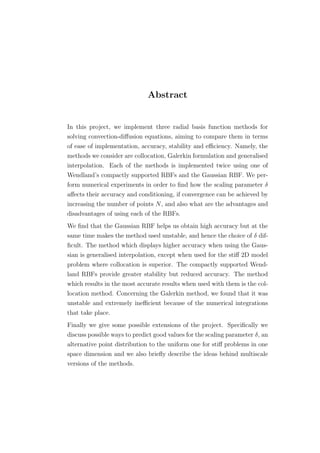
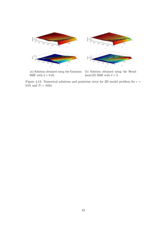
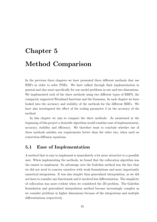
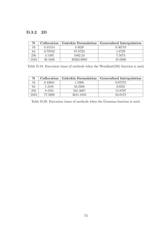
This thesis compares three radial basis function methods - collocation, Galerkin formulation, and generalized interpolation - for solving convection-diffusion equations. Numerical experiments are performed using different radial basis functions and problem sizes to evaluate the methods' ease of implementation, accuracy, stability, and efficiency. The author finds that while the Gaussian radial basis function achieves high accuracy, it also leads to instability. The compactly supported Wendland functions provide greater stability but reduced accuracy. Overall, the collocation method performs best for the compactly supported functions, while generalized interpolation is most accurate when using the Gaussian basis. The Galerkin method is found to be unstable and inefficient. Possible extensions discussed include methods for selecting the scaling parameter and non


![Chapter 1
Introduction
Radial Basis Function (RBF) methods trace their origins back to Hardy’s multi-
quadric (MQ) method [6]. This method was developed by Hardy as a way to obtain a
continuous function that would accurately describe the morphology of a geographical
surface. The motivation came from the fact that the already existing methods at the
time, like Fourier and polynomial series approximations, provided neither acceptable
accuracy nor efficiency [6], [24]. Moreover obtaining the desired result as a continu-
ous function meant that analytical techniques from calculus and geometry could be
utilised to provide useful results, e.g. the height of the highest hill, unobstructed lines
of sight, volumes of earth and others [6].
In mathematical terms, the problem Hardy was trying to solve can be stated
as: given a set of unique points X = {x1, ..., xn} ∈ Rd
with corresponding values
{f1, ..., fn}, find a continuous function s(x) that satisfies the given value at each
point, i.e., s(xi) = fi for i = 1, .., n. Hardy [6], following a trial and error approach,
constructed the approximate solution by taking a linear combination of the multi-
quadric functions
qj(x) = c2 + x − xj
2
2, j = 1, .., n, (1.1)
where each of these functions is centered about one of the unique points in our set.
The problem therefore reduces to finding the coefficients Cj such that
s(xi) =
n
j=1
Cjqj(xi) = fi, i = 1, .., n, (1.2)
which involves nothing more than solving a system of linear equations. It has been
proved that the system of linear equations resulting from the MQ method is always
nonsingular, see for example, Micchelli [12].
1](https://image.slidesharecdn.com/c24706f7-2946-435e-a97b-0f69adf3d631-150222142222-conversion-gate02/85/Thesis_Main-12-320.jpg)
![The MQ method, which has found applications in areas other than topography,
has also been used in order to numerically approximate the solution to partial dif-
ferential equations. In fact, Kansa [9] found, after performing a series of numerical
experiments, that the MQ method in many cases outperformed finite difference meth-
ods, providing a more accurate solution while using a smaller number of points and
without having to create a mesh.
After Micchelli [12] provided the conditions under which the resulting linear sys-
tem of Hardy’s method is nonsingular, it was realised that other functions, as well
as (1.1) could also be used with the method. The common characteristic of those
functions is that their value only depends on the distance from a chosen center, i.e.,
they are radially symmetric with respect to that center. These functions are now
widely known as radial basis functions (RBFs).
1.1 Aim of Thesis
The motivation for looking into radial basis function methods for numerically solv-
ing partial differential equations (PDEs) comes from the fact that standard methods,
like finite differences or finite elements, can easily become computationally expensive.
This is a direct result of the requirement of these methods for creating a mesh, and
also the need for having usually a large number of points in order to obtain accept-
able accuracy. The necessity of using a really small stepsize is more evident when the
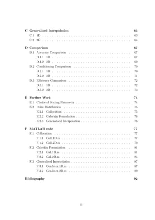
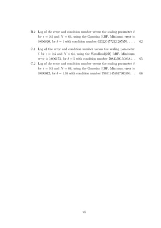
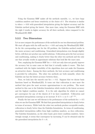
solution to be approximated has stiff regions. For example, in Figure 1.1 we see the
finite element solution on a uniform mesh to both a 1D and a 2D convection domi-
nated diffusion problem where we get oscillations in the boundary layer. Moreover,
Figure 1.1: Numerical solutions obtained using finite element methods.
2](https://image.slidesharecdn.com/c24706f7-2946-435e-a97b-0f69adf3d631-150222142222-conversion-gate02/85/Thesis_Main-13-320.jpg)
![the methods become increasingly complex as we take into consideration problems in
higher dimensions.
Perhaps the greatest advantage of RBF methods is that, in contrast to finite
elements and finite differences, they offer mesh free approximation. Highly important
is also the ease in which these methods can be generalized to higher dimensions. We
only have to consider the Euclidean norm of the distance between a point and the
center of the RBF in order to find its value and therefore, the majority of times, the
same function can be used to solve problems in any dimension.
These two main characteristics of RBFs captured the attention of mathematicians.
Since the time Hardy’s MQ method was first introduced , several algorithms utilizing
different RBFs have been developed, each with its own merits and faults.
An ideal algorithm would combine ease of implementation with high accuracy
and efficiency. The aim of this thesis is the implementation and comparison, in terms
of accuracy and conditioning of the resulting linear system, of three different radial
basis function algorithms for solving convection-diffusion equations in one and two
dimensions. The methods we consider are collocation [8],[9], a Galerkin formulation
method [1],[3],[11],[21] and generalized interpolation [4]. We will implement each of
these methods using two different types of RBFs, an infinitely differentiable one and
two compactly supported functions.
1.2 Radial Basis Functions
As mentioned in the previous section, throughout this project we will make use of
different RBFs when implementing our methods. We consider the infinitely differen-
tiable Gaussian function and two of Wendland’s [19] compactly supported functions
for one and two dimensions. These functions are available in Table 1.1.
Type of RBF φ(r) r ≥ 0 Ck
Gaussian exp(−r2
) C∞
Wendland (1D) (1 − r)5
+(8r2
+ 5r + 1) C4
Wendland (2D) (1 − r)6
+(35r2
+ 18r + 3) C4
Table 1.1: Table of radial basis functions.
We take as the input r for our RBF the Euclidean distance of a point from the
centre of the function, scaled by a scaling parameter δ ∈ R, that is,
r =
x − xj
δ
, j = 1, .., n. (1.3)
3](https://image.slidesharecdn.com/c24706f7-2946-435e-a97b-0f69adf3d631-150222142222-conversion-gate02/85/Thesis_Main-14-320.jpg)
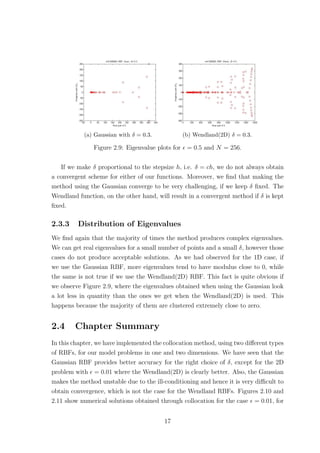
![(a) Gaussian (b) Wendland (1D)
(c) Wendland (2D)
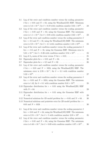
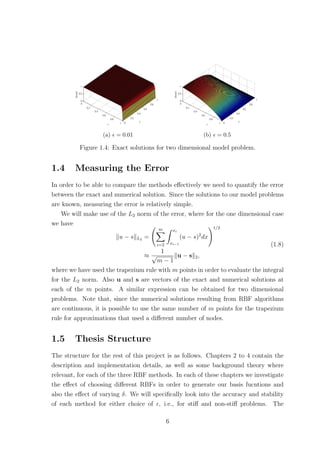
Figure 1.2: Radial basis functions, with centre xj = 4
9
, for different values of δ.
The parameter δ affects the shape of the RBF, as well as the accuracy of the method.
Observing Figure 1.2 we can see that as we increase the scaling parameter δ the
Gaussian RBF flattens out while the support radius of the two Wendland functions
increases. We expect that increasing δ will result in larger condition numbers for our
systems, especially for the Gaussian function which is not compactly supported.
A slight advantage of the Gaussian RBF is the fact that it can be used for ap-
proximations in any dimension, while we need to use a different compactly supported
Wendland function for each dimension. The reason why the same Wendland function
should not be used for any dimension has to do with the positive definiteness of com-
pactly supported functions, such as the Wendland RBFs, being dependent on how
many dimensions we are working with, as stated in [19]. A positive definite function
results in a positive definite linear system for (1.2), which in turns implies that we
can always find a unique solution, as all its eigenvalues are positive.
1.3 Model Problems
In this section we give the model problems on which we will test the different RBF
algorithms. Our 1D convection diffusion equation with Dirichlet boundary conditions
4](https://image.slidesharecdn.com/c24706f7-2946-435e-a97b-0f69adf3d631-150222142222-conversion-gate02/85/Thesis_Main-15-320.jpg)
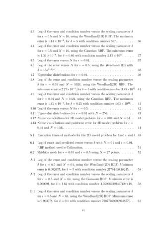
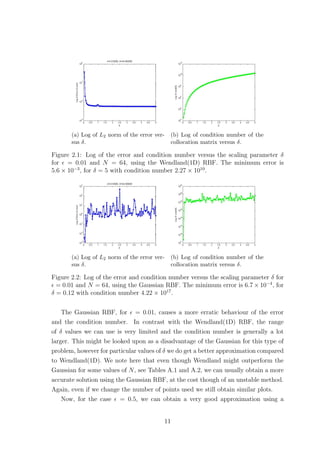
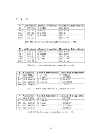
![(a) = 0.01 (b) = 0.5
Figure 1.3: Exact solutions for one dimensional model problem.
is given by
− u + u = 0, 0 < x < 1,
u(0) = 1,
u(1) = 0,
(1.4)
where > 0 is the diffusion coefficient. The exact solution for this problem is
u(x) =
1 − exp(−(1 − x)/ )
1 − exp(−1/ )
. (1.5)
We will also consider a two dimensional problem, again with Dirichlet boundary
conditions. It is given by
− 2
u + (1, 2) · u = 0, (x, y) ∈ Ω,
u(1, y) = 0, y ∈ [0, 1]
u(x, 1) = 0, x ∈ [0, 1]
u(0, y) =
1 − exp(−2(1 − y)/ )
1 − exp(−2/ )
, y ∈ [0, 1],
u(x, 0) =
1 − exp(−(1 − x)/ )
1 − exp(−1/ )
, x ∈ [0, 1],
(1.6)
where again > 0 is the diffusion coefficient and Ω = (0, 1)2
. The exact solution of
the problem is
u(x, y) =
1 − exp(−(1 − x)/ )
1 − exp(−1/ )
1 − exp(−2(1 − y)/ )
1 − exp(−2/ )
. (1.7)
In both cases, varying affects how stiff the solution is and hence how easy it is to
construct an approximation for it, i.e., for small values of our solution becomes stiff
whereas for values close to 1 we have a solution whose gradient is not as steep. We
will perform our numerical experiments for two values of , namely = 0.01 for which
our solutions are stiff and = 0.5 for which the solutions are more well behaved, see
Figures 1.3 and 1.4.
5](https://image.slidesharecdn.com/c24706f7-2946-435e-a97b-0f69adf3d631-150222142222-conversion-gate02/85/Thesis_Main-16-320.jpg)

![Chapter 2
Collocation
2.1 Method Description
Collocation, which was first introduced by Kansa [8], [9], is perhaps the most straight-
forward method amongst the three to be discussed. In order to demonstrate how collo-
cation works, let us first consider the following general convection-diffusion equation,
Lu = − 2
u + b · u + cu = f in Ω ⊆ Rd
u = gD on ∂Ω
(2.1)
where > 0 is the diffusion coefficient and b ∈ Rd
.
The first step of this method is to consider a set of basis functions
Φj(x) = φ
x − xj 2
δ
, j = 1, ..., N, (2.2)
where N is the total number of points we are using and j indicates which node
we are centering around. Note that we are using Φj as a function with a vector
argument and φ as a function with a scalar argument. The set of points used are
known as collocation points. We then form our approximate solution by taking a
linear combination of our basis functions, that is,
s(x) =
N
j=1
CjΦj(x). (2.3)
Substituting s(x) back into our equation and boundary conditions and evaluating at
each of our N points gives,
N
j=1
Cj (− 2
Φj(xi) + b · Φj(xi) + cΦj(xi)) = f(xi) i = 1, ..., N∗
,
N
j=1
Cj Φj(xi) = gD(xi) i = N∗
+ 1, ..., N,
(2.4)
8](https://image.slidesharecdn.com/c24706f7-2946-435e-a97b-0f69adf3d631-150222142222-conversion-gate02/85/Thesis_Main-19-320.jpg)
![where points 1 to N∗
are located within the domain and points N∗
+1 to N lie on the
boundary. We will only consider uniform distributions for all methods in this project,
for comparison purposes. The system of equations (2.4) can be written as a matrix
equation of the form
AC = F (2.5)
where
A =
Lφ
φ
, C =
C
, F =
f
gD
. (2.6)
The matrix A has dimensions N × N and F, C are N dimensional vectors. The
method is also known as unsymmetric collocation [7] because of the non symmetric
collocation matrix A. Note that the matrix A is not symmetric even if the PDE is
self-adjoint. In order to acquire the unknown coefficients Cj we must solve Equation
(2.5) for C. It is therefore important that the collocation matrix is nonsingular for
this method to work.
In the case of a simple interpolation problem, see (1.2), this method may some-
times yield singular collocation matrices for specific RBFs [7], like Thin Plate Splines
for which φ(r) = r2
log(r). This can be fixed by adding an extra polynomial to (2.3)
and imposing additional constraints on the coefficients Cj in order to eliminate the
additional degrees of freedom. However, it has been proven that this is not the case
for elliptic problems. Hon and Schaback [7] have managed to construct examples
where the collocation matrix becomes singular, whether you add the extra appropri-
ate polynomial or not.
In particular, Hon and Schaback [7], have managed to find, relatively easily, cases
where using the Gaussian RBF results in a singular collocation matrix. Numerical
experiments were performed with Wendland functions as well but a singular colloca-
tion matrix was not found. However, Hon and Schaback do not believe that using the
compactly supported Wendland functions will always result in a nonsingular system
of equations. This indicates however that we should probably expect better condi-
tioning when using the Wendland RBFs, compared to the Gaussian. We also note
that we will not be considering any additional polynomial terms in our approximate
solution because, as stated by [10] and [2], they do not offer any significant benefits
with regards to the accuracy of the method.
In the following sections of this chapter we will apply the method to our model
problems in one and two dimensions, for different values of , using the Wendland
and Gaussian RBFs. The aim is to look into which of the two RBFs perform better
9](https://image.slidesharecdn.com/c24706f7-2946-435e-a97b-0f69adf3d631-150222142222-conversion-gate02/85/Thesis_Main-20-320.jpg)
![Gaussian Wendland (1D) Wendland (2D)
φ(r) exp(−r2
) (1 − r)5
+(8r2
+ 5r + 1) (1 − r)6
+(35r2
+ 18r + 3)
φ (r) −2r exp(−r2
) (1 − r)4
+(−56r − 14r) (1 − r)5
+(−280r2
− 56r)
φ (r) (−2 + 4r2
) exp(−r2
) (1 − r)3
+(336r2
− 42r − 14) (1 − r)4
+(1960r2
− 224r − 56)
Table 2.1: Derivatives of RBFs.
in terms of conditioning of the collocation matrix and accuracy of the solution. Also
of interest is how the value of the scaling parameter δ affects the method.
2.2 One Dimension
Having explained how the collocation method works, we will now apply it to our 1D
problem (1.4). Prior to coding the method in MATLAB, we must first calculate the
first and second derivatives of φ with respect to x, that is
dΦj
dx
=
1
δ
dφ
dr
if x > xj
−1
δ
dφ
dr
if x < xj
,
d2
Φj
dx2
=
1
δ2
d2
φ
dr2
, (2.7)
where the derivatives of φ with respect to r can be found in Table 2.1. The translation
of the collocation method to a computer program is relatively simple, which is one of
the reasons why this method became popular.
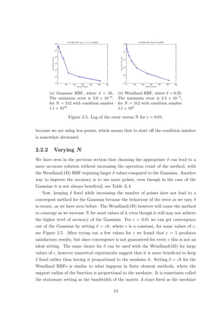
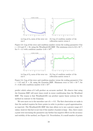
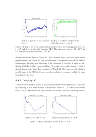
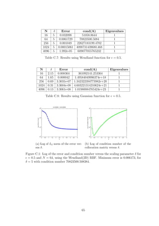
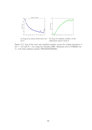
2.2.1 Scaling Parameter δ
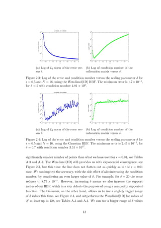
The scaling parameter δ is known to affect the accuracy of RBF based methods.
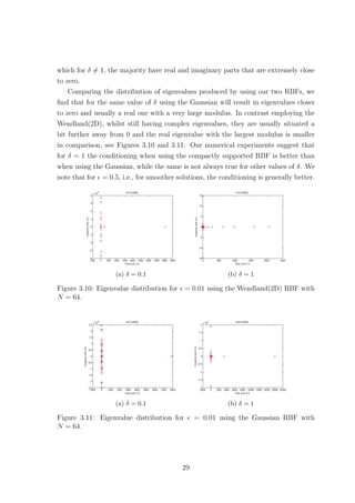
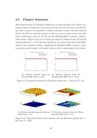
Figures 2.1 and 2.2 show how the error and condition number get affected when we
vary δ, for the Wendland(1D) and Gaussian RBFs respectively, where = 0.01. The
Wendland(1D) RBF seems to provide us with exponential convergence as we increase
δ. However as the error decreases the condition number of the method increases. This
implies that as we increase δ the method becomes unstable due to the ill-conditioning
of the collocation matrix. Something similar was also observed for plain interpolation
problems, where as mentioned in Schaback [15],‘either one goes for a small error and
gets a bad sensitivity, or one wants a stable algorithm and has to take a comparably
larger error’. As far as the Wendland(1D) case of the method is concerned, for
= 0.01, we observe that after some point increasing δ any further does not have a
significant impact on the accuracy while it still affects the condition number. This
suggests that it might be worth sacrificing a bit of accuracy for a more stable method.
Changing the number of points does not affect the behaviour observed in Figure 2.1.
10](https://image.slidesharecdn.com/c24706f7-2946-435e-a97b-0f69adf3d631-150222142222-conversion-gate02/85/Thesis_Main-21-320.jpg)
![Chapter 3
Galerkin Formulation
3.1 Galerkin Method for Robin Problems
The second method we consider is based on a Galerkin formulation of the problem.
It is somewhat similar to a finite element method with the distinct difference that we
do not need to perform a computationally expensive mesh generation. Of course the
basis functions used in our case are radially symmetric.
Wendland [21], looked into a Galerkin based RBF method for second order PDEs
with Robin boundary conditions, for an open bounded domain Ω having a C1
bound-
ary, that is,
−
d
i,j=1
∂
∂xi
aij
∂u
∂xj
(x) + c(x)u(x) = f(x), x ∈ Ω,
d
i,j=1
aij(x)
∂u(x)
∂xj
νi(x) + h(x)u(x) = g(x), x ∈ ∂Ω,
(3.1)
where aij, c ∈ L∞(Ω), i, j = 1, ..., n, f ∈ L2(Ω), aij, h ∈ L∞(∂Ω), g ∈ L2(∂Ω) and
ν is the outward unit normal vector to ∂Ω. The entries aij(x) satisfy the following
ellipticity condition, namely, there exists a constant γ > 0 such that for all x ∈ Ω
and all α ∈ Rd
γ
d
j=1
α2
j ≤
d
i,j=1
aij(x)αiαj. (3.2)
As stated in [21], under the additional assumption that the functions c and h are
both non-negative and one or both of them are ‘uniformly bounded away from zero
on a subset of nonzero measure of Ω for c or ∂Ω for h, we obtain a strictly coercive
and continuous bilinear functional’
a(u, v) =
Ω
d
i,j=1
aij
∂u
∂xj
∂v
∂xi
+ cuv dx +
∂Ω
huv dS ∈ V × V, (3.3)
19](https://image.slidesharecdn.com/c24706f7-2946-435e-a97b-0f69adf3d631-150222142222-conversion-gate02/85/Thesis_Main-30-320.jpg)
![where V = H1
(Ω). Combining a(u, v) with the continuous linear functional l(v) ∈ V ,
where
l(v) =
Ω
fvdx +
∂Ω
gvdS, (3.4)
we obtain the weak formulation of the problem,
find u ∈ V such that a(u, v) = l(v) holds for all v ∈ V, (3.5)
which by the Lax-Milgram theorem is always uniquely solvable.
The next step is to consider a finite dimensional subspace VN ⊂ V spanned by
our RBFs, that is,
VN := span{Φj(x), j = 1, ..., N} (3.6)
for a set of pairwise distinct points X = {x1, ..., xN} ∈ Ω, and search for an approx-
imation s ∈ VN to u that satisfies a(s, v) = l(v) for all v ∈ VN . It is mentioned in
[21] that is preferable to use compactly supported functions, such as the Wendland
RBFs, in order to obtain some sparsity in the resulting matrix. Wendland provided
the theoretical bounds for such settings. We give below a special case of Theorem
5.3, with m = 0, proved in [21].
Theorem 3.1.1.
Assume u ∈ Hk
(Ω) and Φ is such that its Fourier transform satisfies ˆΦ(ω) ∼ (1 +
ω 2)−2σ
with σ ≥ k > d/2. Then there exists a function s ∈ VN , such that
u − s L2(Ω) ≤ Cˆhk
u Hk(Ω),
for sufficiently small ˆh = supx∈Ω min1≤j≤N x − xj 2.
The Wendland RBFs satisfy the requirements of the theorem with σ = 3 and
σ = 3.5, for the 1D and 2D versions respectively. Also, ˆh corresponds to the data
density or mesh norm as stated in [4] that ‘measures the radius of the largest data-free
hole contained in Ω’.
3.2 Galerkin Method for the Dirichlet Problem
In our case, both model problems have Dirichlet boundary conditions. This poses a
difficulty for Galerkin methods as they cannot simply be used with RBFs, as men-
tioned in [1]. As the boundary conditions need to be satisfied by the space in which
the solution u belongs [1], [3], a problem arises because RBFs, even compactly sup-
ported ones, do not satisfy these boundary conditions in general. Therefore the error
bound given in Theorem 3.1.1, is most likely, not valid in our case.
20](https://image.slidesharecdn.com/c24706f7-2946-435e-a97b-0f69adf3d631-150222142222-conversion-gate02/85/Thesis_Main-31-320.jpg)
![Different methods have been developed to tackle problems with Dirichlet boundary
conditions, including approximating the Dirichlet problem by an appropriate Robin
problem [1], using a Lagrange multiplier approach [3] and others [11]. We will follow a
quite different approach by adding additional terms to our weak formulation in order
to impose the boundary conditions.
The weak formulation of the general convection-diffusion problem (2.1) is to find
u ∈ H1
E(Ω) such that
Ω
u · v + b · uv + cuv dΩ −
∂Ω
v
∂u
∂ν
dS =
Ω
fv dΩ (3.7)
for all v ∈ H1
E0
(Ω), where H1
E(Ω) = {ω| ω ∈ H1
(Ω), ω = gD on ∂Ω} and H1
Eo
(Ω) =
{ω| ω ∈ H1
(Ω), ω = 0 on ∂Ω}. Note here that the boundary terms vanish since
v ∈ H1
Eo
(Ω). However, as we have pointed out earlier our RBFs span VN which is a
subspace of H1
(Ω) and therefore cannot be used in this setting. In order to impose
the boundary conditions we consider the following relation
∂Ω
θ
∂v
∂ν
+ κv u dS =
∂Ω
θ
∂v
∂ν
+ κv gD dS, (3.8)
where θ ∈ [−1, 1] and κ = c/h, which we incorporate in (3.7). Note that here h
is the meshsize, which is constant as we are using a uniform distribution. Our new
formulation of the problem is,
find u ∈ H1
(Ω) such that a(u, v) = l(v) holds for all v ∈ H1
(Ω), (3.9)
where
a(u, v) =
Ω
u · v + b · uv + cuv dΩ −
∂Ω
v
∂u
∂ν
dS
+
∂Ω
θ
∂v
∂ν
+ κv u dS
l(v) =
Ω
fv dΩ +
∂Ω
θ
∂v
∂ν
+ κv gD dS.
(3.10)
The idea of imposing the boundary conditions in a weak sense, like we have done
here, has been discussed in [16] for finite element methods. After a few numerical
experiments we have found that choosing θ = −1 and κ = 5/h produces more accurate
results the majority of time. Setting θ = −1 means that the symmetric part of the
elliptic operator will correspond to a symmetric bilinear form.
We construct the approximate solution s ∈ VN by taking a linear combination of
our basis functions, that is,
s(x) =
N
j=1
CjΦj(x) (3.11)
21](https://image.slidesharecdn.com/c24706f7-2946-435e-a97b-0f69adf3d631-150222142222-conversion-gate02/85/Thesis_Main-32-320.jpg)
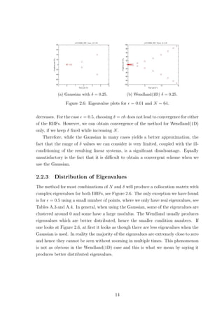
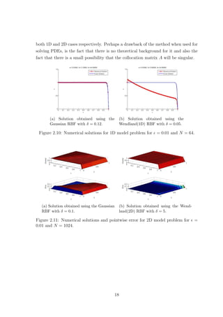
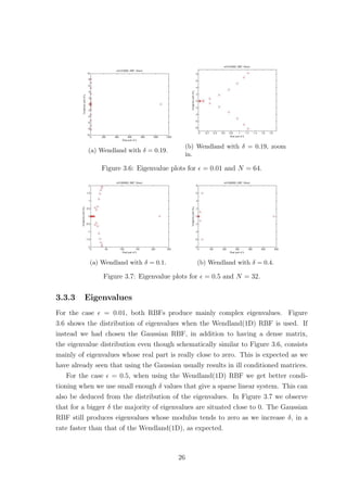
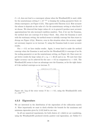
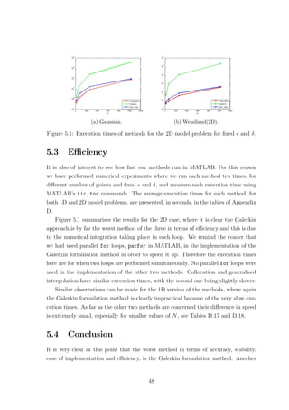
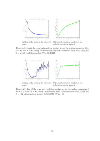
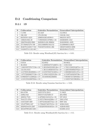
![(a) Wendland(1D) with δ = 0.2. (b) Gaussian with δ = 0.25.
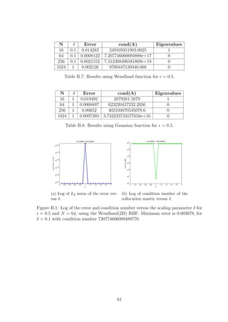
Figure 3.5: Log of L2 norm of the error versus N for = 0.01.
is used, the choice of δ is not as tricky as when = 0.01. Now for the Gaussian,
even though the choice of δ is a bit more difficult, see Figure 3.4, the accuracy of the
method is clearly better, even though more unstable, for most values of N, see Tables
B.3 and B.4.
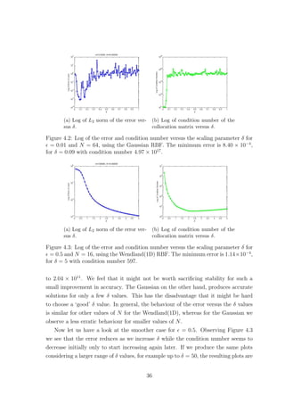
3.3.2 Increasing the number of points N
It should be possible to achieve convergence of the method by increasing the number
of points used. We remind the reader that we are always using uniformly distributed
points. As can be observed from the tables in Appendix B, values of δ that work well
with a specific number of points, do not necessarily result in an accurate scheme if
we change N. This is an issue if one wishes to obtain convergence by increasing the
number of points used. After a few numerical experiments we realise that keeping δ
fixed while increasing N does not guarantee convergence for either RBF, see Figure
3.5. Also, for compactly supported functions, such as the Wendland(1D) RBF, using
an increasingly smaller stepsize h while keeping the support fixed, eliminates the
advantage of having sparse matrices [20]. The fact that we cannot obtain convergence
by increasing N confirms that Theorem 3.1.1 does not hold in our setting.
The other choice we have would be to take δ to be proportional to h. This choice
would potentially keep the sparsity of the resulting linear systems if a compactly
supported function is used. However numerical experiments suggest that convergence
is unattainable in this setting too. This was also observed in [20] where the Helmholtz
equation is considered.
25](https://image.slidesharecdn.com/c24706f7-2946-435e-a97b-0f69adf3d631-150222142222-conversion-gate02/85/Thesis_Main-36-320.jpg)
![Chapter 4
Generalised Interpolation
The final method we will discuss is called generalised interpolation. This method is
unique in the sense that it results in symmetric collocation matrices which are also
positive definite for constant coefficient PDEs when positive definite RBFs are used
[22].
Wendland in [22] has managed to provide bounds for the smallest eigenvalue of this
method for general boundary value problems, while in [4] a bound on the condition
number is provided for strictly elliptic PDEs with Dirichlet boundary conditions, i.e.,
for
Lu =f in Ω,
u =gD on ∂Ω,
(4.1)
where
Lu(x) =
d
i,j=1
aij(x)
∂2
∂xi∂xj
u(x) +
d
i=1
bi(x)
∂
∂xi
u(x) + c(x)u(x), (4.2)
and the coefficients aij(x) satisfy the ellipticity condition (3.2). These results however
hold only for a specific type of RBFs. As the setting discussed in [4] is closer to our
model problems we will focus on it.
4.1 Method Description
Before moving on to the convergence and stability results , in this section, we provide
the reader with a description of the method. To start off, we define the functionals
λi as follows
λi(u) = Lu(xi) if xi ∈ Ω,
λi(u) = u(xi) if xi ∈ ∂Ω.
(4.3)
For generalised interpolation, we construct our approximation s to the solution u in
a slightly different way than the previous two methods. The approximation s to the
31](https://image.slidesharecdn.com/c24706f7-2946-435e-a97b-0f69adf3d631-150222142222-conversion-gate02/85/Thesis_Main-42-320.jpg)
![exact solution u, this time is given by
s(x) =
N
j=1
Cjλχ
j φ
x − χ 2
δ
, (4.4)
where this time our RBF depends on two variables x and χ. Note that we have
applied the functional λj to the function φ with respect to the new argument χ. In
this chapter we redefine Φ as a function of two vector arguments, that is,
Φ(x, χ) = φ(r),
where r = x−χ 2
δ
. As always, we are using N uniformly distributed points in order
to simplify the comparison process. We then substitute our expression for s(x) back
into the PDE and boundary conditions or equivalently apply the functional λi to s
with respect to x, that is,
λx
i (s) = fi, i = 1, ..., N, (4.5)
where
fi = f(xi) if xi ∈ Ω,
fi = gD(xi) if xi ∈ ∂Ω.
(4.6)
This can be rewritten as a matrix equation
AC = F, (4.7)
where the entries of the symmetric collocation matrix A are given by
Ai,j = λx
i λχ
j φ
x − χ 2
δ
, (4.8)
and the entries of the right-hand-side vector F are given by Fi = fi. Solving the
matrix Equation (4.7) will provide us with the unknown coefficients Cj and hence the
approximate solution s(x).
4.2 Stability and Accuracy
We first need to give the definition of the fractional Sobolev space Wσ
2 (Rd
). As stated
in [4] ‘we describe functions in the fractional Sobolev space Wσ
2 (Rd
) as those square
integrable functions that are finite in the norm
f 2
Wσ
2 (Rd) =
Rd
| ˆf(ω)|2
(1 + ω 2
2)σ
dω, (4.9)
where ˆf is the usual Fourier transform’. We note here that σ can be both an integer
and a fraction. Also needed is the definition of a reproducing kernel to a Hilbert
space, which is given below as found in [4].
32](https://image.slidesharecdn.com/c24706f7-2946-435e-a97b-0f69adf3d631-150222142222-conversion-gate02/85/Thesis_Main-43-320.jpg)
![Definition 4.2.1. (Reproducing Kernel)
Suppose H ⊂ C(Ω) denotes a real Hilbert space of continuous functions f : Ω → R;
then Φ : Ω × Ω → R is said to be a reproducing kernel for H if
• Φ(·, χ) ∈ H for all χ ∈ Ω
• f(χ) = (f, Φ(·, χ))H for all f ∈ H and all χ ∈ Ω.
Both of our RBFs are reproducing kernels to a Hilbert space, also know as the
native space of the RBF [5]. We now move on to the main stability result proven
in [4]. It is important here to notice that the result only holds for the Wendland
RBFs which are compactly supported reproducing kernels. As we will also see from
numerical experiments in the following sections, this result does not apply to the
Gaussian RBF.
Theorem 4.2.1.
Suppose Wσ
2 (Rd
) with σ > d/2+2 has a compactly supported reproducing kernel, Φ,
which has a Fourier transform satisfying
c1(1 + ω 2
2)−σ
≤ ˆΦ(ω) ≤ c2(1 + ω 2
2)−σ
.
Let 0 < δ ≤ 1. Suppose L is a linear, strictly elliptic, bounded, second order differ-
ential operator. Then for sufficiently small δ the condition number of the collocation
matrix A can be bounded by
cond(A) ≤ Cδ−4
1 +
2δ
h
d
δ
h
2σ−d
with a constant C independent of h and δ.
The bound on the condition number of A is derived from the bounds
λmin ≥ C1
h
δ
2σ−d
,
λmax ≤ C2δ−4
1 +
2δ
h
d
,
(4.10)
where λmax and λmin are respectively the maximum and minimum eigenvalues of A
and C1, C2 > 0 are independent of h and δ. It is proved in [19], that Wendland(1D)
and Wendland(2D) RBFs satisfy the conditions of Theorem 4.2.1 with σ = 3 and
σ = 3.5 respectively.
Wendland and Farrell in [4] have also provided a bound on the L2 norm of the
error. We give below Lemma 4.4 which is stated and proven in [4].
33](https://image.slidesharecdn.com/c24706f7-2946-435e-a97b-0f69adf3d631-150222142222-conversion-gate02/85/Thesis_Main-44-320.jpg)
![Gaussian Wendland (1D) Wendland (2D)
φ (r) −4r(2r2
− 3)e−r2
(1 − r)2
+(−1680r2
+ 840r) (1 − r)3
+(5040r −
11760r2
)
φiv
(r) (12 − 48r2
+ 16r4
)e−r2
(1 − r)+(6720r2
− 5880r + 840) 1680(1 − r)2
+(5r −
3)(7r − 1)
Table 4.1: Derivatives of RBFs.
Theorem 4.2.2. (L2−error)
Assume δ ∈ (0, 1]. Let u ∈ Hσ
(Ω) be the solution of (4.1). Let the domain Ω have a
Ck,s
boundary for s ∈ (0, 1] such that σ = k + s and k := σ > 2 + d/2. Then the
error between the solution u and its generalised interpolation approximation s can be
bounded in the L2 norm by
u − s L2(Ω) ≤ Cδ−σ
hσ−2
u Hσ(Ω),
where h = supx∈Ω min1≤j≤N x − xj 2.
In the original version of the theorem, h is the maximum between the mesh norm
of the points in Ω and the mesh norm of the points on the boundary ∂Ω. In our case
we have uniformly distributed points so h can be taken to simply be the meshsize.
The definition of a Ck,s
boundary is given in [23], Definition 2.7.
In our numerical experiments we will consider three cases for δ, the stationary
setting δ = ch, the nonstationary setting δ = ch1−2/σ
and also keeping δ fixed. We
note that the nonstationary setting will only be considered for the Wendland RBFs.
4.3 One Dimension
Prior to coding the method for our 1D model problem in MATLAB, we need to
calculate the appropriate derivatives. Let Gj = λχ
j φ(|x−χ|
δ
) for j = 1, ..., N where
Gj(x) = −
∂2
Φ
∂χ2
+
∂Φ
∂χ χ=xj
, j = 2, ..., N − 1,
Gj(x) = φ
|x − xj|
δ
, j = 1, N,
(4.11)
and
∂Φ
∂χ
=
−1
δ
dφ
dr
if x > χ
1
δ
dφ
dr
if x < χ
,
∂2
Φ
∂χ2
=
1
δ2
d2
φ
dr2
. (4.12)
We can then write s(x) = N
j=1 CjGj(x) which we essentially substitute back into
the PDE and boundary conditions. We therefore need to calculate up to the fourth
34](https://image.slidesharecdn.com/c24706f7-2946-435e-a97b-0f69adf3d631-150222142222-conversion-gate02/85/Thesis_Main-45-320.jpg)
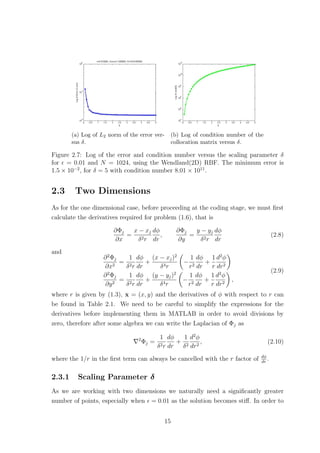
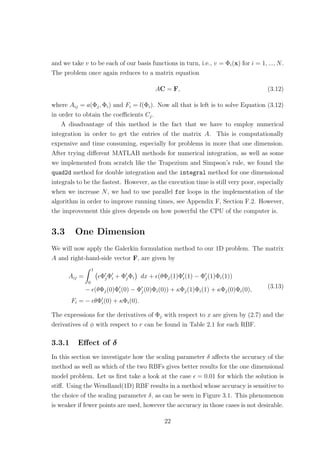
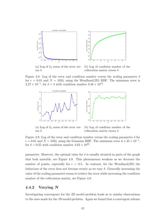
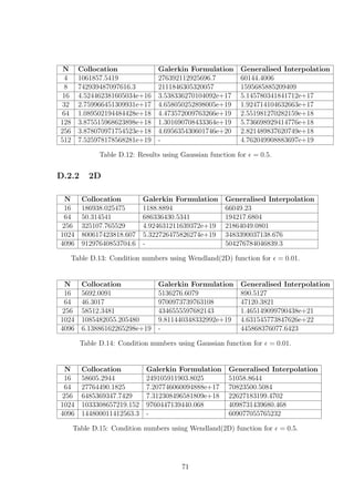
![(a) Gaussian with δ = 0.25. (b) Wendland(1D) with δ = 0.25.
Figure 4.7: Eigenvalue distributions for = 0.01.
and C.3. The Gaussian however, for up to a certain number of points yielded real
eigenvalues some of which were negative and extremely close to zero. Increasing N
further caused complex eigenvalues with very small imaginary parts to appear, see
Tables C.2 and C.4. This fact confirms that using the Wendland(1D) function pro-
duces a positive definite collocation matrix. However our numerical findings suggest
this is not the case if we use the Gaussian RBF, see Figure 4.7. Since the colloca-
tion matrix A is always symmetric this implies that the eigenvalues should always
be real. Therefore the imaginary parts must be due to rounding errors either in the
computation of the matrix entries or in the computation of the eigenvalues. In fact
the matrix A should be positive definite [4], so the negative eigenvalues must also be
an artifact. Nevertheless, the smallest Gaussian eigenvalues are significantly smaller
than the smallest Wendland ones.
Now, as far as the bounds given by (4.10) are concerned we found that they
were satisfied when the Wendland(1D) was used, for all the different values of N we
considered and δ ∈ (0, 1], for both values of . Of course there is no reason to check
these bounds for the Gaussian as they only apply to compactly supported RBFs.
4.4 Two Dimensions
Generalised interpolation requires us to calculate up to the fourth derivative of our
RBFs, therefore it can only be used with RBFs that at least belong in C4
. Another
drawback that becomes obvious when the method is used for higher dimensions, is the
need to basically apply the PDE twice, which complicates the process significantly
even in just two dimensions.
39](https://image.slidesharecdn.com/c24706f7-2946-435e-a97b-0f69adf3d631-150222142222-conversion-gate02/85/Thesis_Main-50-320.jpg)
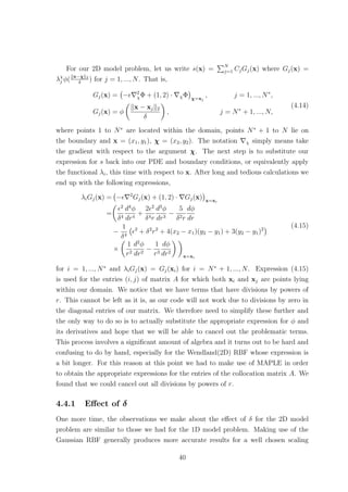
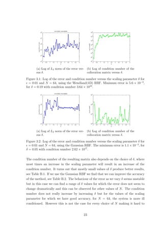
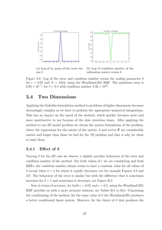
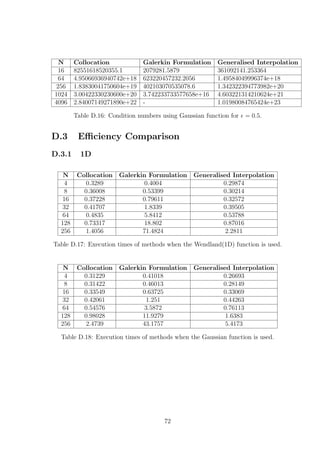
![(a) Gaussian with δ = 10h.
(b) Wendland(2D) with
δ = 10h1−2σ.
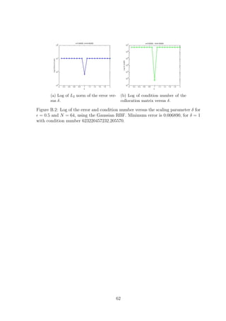
Figure 4.10: Log of the error versus N for = 0.5.
could only be obtained for = 0.01 if the compactly supported Wendland(2D) RBF
was used with a fixed δ or with δ = ch1−2/σ
, where σ = 3.5. As before, increasing c
seems to help us achieve better accuracy. Once more, our findings agree with Theorem
4.2.2.
In our numerical experiments for = 0.5, however, we found that the Gaussian
could produce a convergent scheme for δ = ch, providing us with better accuracy than
the Wendland(2D) RBF, see Figure 4.10. Of course this increased accuracy that the
Gaussian RBF provides us with goes together with an enormous condition number.
4.4.3 Eigenvalues
Experimenting with various values for N we see that as for the 1D case using the
Wendland(2D) produces a collocation matrix with only real and positive eigenvalues
for both = 0.01 and = 0.5. Furthermore, we found that these eigenvalues satisfied
the bounds given by (4.10) for δ ∈ (0, 1].
Now if we use the Gaussian RBF, in contrast to the 1D case, we only found real
eigenvalues in all our numerical experiments. However the majority of times some of
them were negative, even though with a very small modulus. The largest in modulus
negative eigenvalue in Figure 4.11(a) is −1.74×10⁻¹³
. Now, since the matrix is again
theoretically positive definite, we believe that the negative eigenvalues appear due to
rounding errors, as for the 1D model problem. This confirms, however, that similar
bounds to (4.10) cannot be obtained when we use translates of the Gaussian RBF as
our basis functions, as we had also deduced for the 1D case.
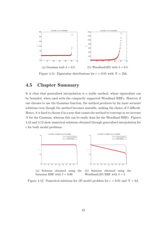
42](https://image.slidesharecdn.com/c24706f7-2946-435e-a97b-0f69adf3d631-150222142222-conversion-gate02/85/Thesis_Main-53-320.jpg)
![thing that can be added to the list of disadvantages of this method, is the difficulty
of applying it to problems with Dirichlet boundary conditions.
Now in terms of accuracy, we have seen that collocation performs better than gen-
eralised interpolation in all cases, when the Wendland RBFs are used. The opposite
is true when we make use of the Gaussian RBF, providing better accuracy at the cost
of instability.
The choice therefore seems to depend on what one regards as more important,
stability or accuracy. If the highest accuracy is required, then the Gaussian RBF
should be chosen and since all methods are more or less unstable for this choice of
RBF, we might as well choose the one that gives the most accurate solution, i.e.,
generalised interpolation. However we note here that for the stiff version of the
2D model problem, collocation was the only method that could produce acceptable
accuracy for both RBFs.
Now, if one is willing to sacrifice a bit of accuracy in order to have stability and
therefore make the choice of δ easier, the Wendland RBFs should be chosen. The
most accurate method when the Wendland RBFs are used is collocation.
Concluding, our personal choice would be the collocation method used with the
Wendland RBFs, especially for stiff problems. It is the most efficient and easy to
implement out of the three and also provides us with convergence as we increase the
number of points. Its only drawbacks is that the collocation matrix A might not
always be invertible, however as mentioned in [7] these cases are rare. Also, the lack
of theory for collocation, as opposed to the other two approaches, might also be seen
as a disadvantage, even though in the case of the Galerkin method the theory is not
really applicable.
49](https://image.slidesharecdn.com/c24706f7-2946-435e-a97b-0f69adf3d631-150222142222-conversion-gate02/85/Thesis_Main-60-320.jpg)
![Chapter 6
Further Work
6.1 Extension: Choice of the Scaling Parameter
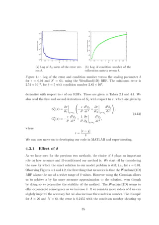
We have observed throughout this project that the choice of the scaling parameter
plays an important role in the accuracy of all three methods. We were able to find
the optimal values of δ because the exact solution to our model problems was known.
However this will not be the case when the algorithms are used in practice. It would
therefore be very useful if there was a way to predict which value of δ should be used.
Mongillo in [13] investigates the use of ‘predictor functions’ whose behaviour is similar
to that of the interpolation error, in the case of collocation used for plain interpolation
problems. The optimal parameter δ is chosen by minimizing these predictor functions.
Uddin in [18] has tried one of these ‘predictor functions’, more specifically the
‘Leave One Out Cross Validation’ (LOOCV), in the context of Collocation applied to
time-dependent PDEs. As also mentioned in [13], for LOOCV we use N − 1 points,
out of the total of N points, in order to compute the solution. We then test the error
at the point we have left out. That is we have,
LOOCV (δ) =
N
i=1
|si(xi) − fi|2
, (6.1)
where si is the approximate solution evaluated at N − 1 points by leaving out the
ith
point and fi is the exact value at points xi. This is repeated N times leaving
out a different point every time. As one might imagine, this procedure increases
the computational complexity of the algorithm, as we have to solve N systems of
equations. This drawback can be eliminated using Rippas algorithm, [14] through [13],
which is also the version of LOOCV algorithm used in [18]. What Rippa essentially
showed was that it is not necessary to solve N linear systems as we have,
si(xi) − fi =
Ci
A−1
ii
. (6.2)
50](https://image.slidesharecdn.com/c24706f7-2946-435e-a97b-0f69adf3d631-150222142222-conversion-gate02/85/Thesis_Main-61-320.jpg)
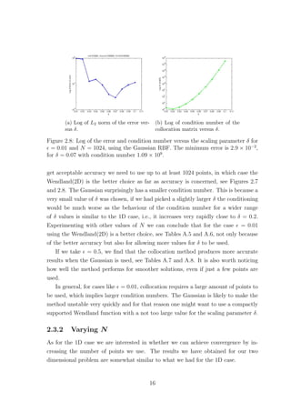
![(a) Gaussian. (b) Wendland(1D).
Figure 6.1: Log of exact and predicted errors versus δ with N = 64 and = 0.01.
RBF method used is Collocation.
As stated in [13], using Rippas algorithm reduces the computational complexity to
O(N3
) rather than O(N4
), which is the complexity for solving a dense linear system
of equations.
Uddin’s numerical experiments have shown that Rippa’s algorithm is not very
useful when used for time-dependent PDEs. Even though in some cases the results
were fairly good, in general the numerical experiments have shown that it does not
always predict good values for δ. Nevertheless, looking into how well this algorithm,
and more generally ‘predictor functions’, perform for the methods we have used in
this project is a topic that requires further work and study.
Here, we have implemented Rippa’s algorithm for all three methods using both
RBFs. Detailed results can be found in Appendix E for the 1D model problem.
Figure 6.1 shows the behaviour of the exact error and the error predictor function
obtained through LOOCV. We can see that the predictor function mimics the error
behaviour best when the Gaussian RBF is used. However our numerical experiments
seem to agree with Uddin’s findings for time-dependent PDES, i.e., even though in
some cases this algorithm gives good results, see Table E.3, in general it is not a
very reliable way to predict δ. As already mentioned in this section, further work in
finding trustworthy methods for predicting δ is required.
6.2 Extension: Point Distribution
Another interesting extension to this project would be to investigate how the methods
perform when non uniform distributions are used. We have seen that a uniform
distribution is perfectly adequate when the solution to be approximated is smooth,
i.e., in our case for = 0.5. However, for stiff problems like for = 0.01, we saw that
51](https://image.slidesharecdn.com/c24706f7-2946-435e-a97b-0f69adf3d631-150222142222-conversion-gate02/85/Thesis_Main-62-320.jpg)
![a much greater number of points was required in order to obtain acceptable levels of
accuracy. This fact provides the motivation to look into other type of meshes.
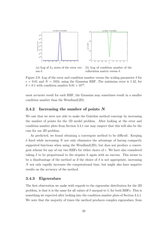
In this section, we will briefly look at the Shishkin mesh [17] and how it affects
the accuracy of the methods when applied to our 1D model problem. A Shishkin
mesh requires an odd number of points N, or equivalently an even number of mesh
spacings M = N − 1. Then, for an equation of the form
− u + bu = 0,
with constant b > 0, a Shishkin mesh consists of M/2 equal mesh spacings in the
interval [0, 1 − σ] and M/2 equal mesh spacings in the interval [1 − σ, 1], where
σ = min(1/2, 2 log(N)/b). (6.3)
For our model problem we have b = 1. We note here that when σ = 0.5 then the
Shishkin mesh reduces to a uniform distribution of the points, see Figure 6.2. This
is the case when = 0.5, therefore we will consider the case for = 0.01. A question
that naturally arises at this point is whether the value of δ should be the same for all
our basis functions. In order to answer this question we will perform our experiments
trying out different values of δ in each of the two differently scaled sections of the
interval [0, 1].
Carrying out our numerical experiments requires us to adjust our code in order to
admit two values for the scaling parameter δ instead of one, i.e., we now have δ = δ1
in the first part of the interval and δ = δ2 in the second part. We then repeatedly
solved our model problem each time using different combinations for our δ values,
for both RBFs and all three methods. We then picked out, for each method and
(a) Shiskin mesh for = 0.5 is just a
uniform distribution.
(b) Shishkin mesh for = 0.01 splits
the interval in two.
Figure 6.2: Shishkin mesh for = 0.01 and = 0.5 using N = 27 points.
52](https://image.slidesharecdn.com/c24706f7-2946-435e-a97b-0f69adf3d631-150222142222-conversion-gate02/85/Thesis_Main-63-320.jpg)
![RBF, the two δ values, amongst those considered, for which the approximate solution
displayed the lowest error. Detailed results form these experiments can be found in
Appendix E, Section E.2.
We found that using the Shishkin mesh in almost all cases considerably reduces
the error. Exceptions are for the collocation method with both RBFs and generalised
interpolation for the Gaussian, where for N = 9 and N = 27 the error actually
increases. However we feel that this might be avoided if we consider more δ values
from the same interval. We observe that for the Galerkin formulation method, using
the Shishkin mesh leads to reductions in the error as great as 99%, for example for the
Gaussian RBF for N = 27 which is the smaller error produced by any combination
of method and RBF for this many points. The most accurate solution, however, is
produced by collocation using the Wendland(1D) RBF for N = 243. It is also worth
noting that in most cases we have δ2 < δ1. Moreover, we observe that in general
the Shishkin mesh with the two different values for δ produces more ill-conditioned
systems than a uniform distribution does.
It is clear that a non uniform distribution of points might be beneficial for stiff
problems, however it does complicates RBF methods especially with respect to how
δ should be chosen. It would be interesting to look into how different distributions
affect the accuracy and also the stability of each of the methods, and whether some
of those methods work better for particular meshes. Without any doubt, alternative
meshes and specifically the Shishkin mesh are worthy of further research.
6.3 Extension: Multilevel Algorithms
Finally, a possible extension would be to look into how well the multilevel versions of
the three methods perform. In general, a multilevel algorithm consists of solving the
same problem on each level and only changing the right hand side. As mentioned in
[20], ‘on each level the residual of the previous level is interpolated’.
The multilevel version of generalized interpolation is investigated in [4] as a way
to overcome the problem of ill-conditioning of the collocation matrix A. This version
of the method is known to converge for δ = ch1−2/σ
. A multilevel algorithm, based
on a Galerkin formulation method, has also been proposed for the solution of PDEs
with Neumann boundary conditions in [20]. In that paper, the multilevel algorithm
is investigated as a solution to the problem of obtaining a convergent scheme and at
the same time not eliminating the sparsity of the matrix A. The multilevel versions
have been investigated theoretically in [4] and [20].
53](https://image.slidesharecdn.com/c24706f7-2946-435e-a97b-0f69adf3d631-150222142222-conversion-gate02/85/Thesis_Main-64-320.jpg)


![= 0.5 δ Error Predicted δ Error
Collocation 0.31 3.9171e-08 0.46 1.0208e-06
Galerkin 0.17 2.3076e-06 0.11 1.8138e-05
Gen. Interpolation 0.43 4.3992e-09 0.49 2.7605e-08
Table E.4: Results for the actual δ for which the error is minimised and for the
predicted δ with the corresponding error. RBF used is the Gaussian with N = 32 for
= 0.5.
E.2 Point Distribution
This section contains results from all three methods, for both RBFs, when used with
a Shishkin mesh to solve the 1D problem with = 0.01. Note that we have two
values of δ here, δ1 corresponds to the value of δ used in the interval [0, 1 − σ] and
δ2 is used in the interval (1 − σ, 1]. The U.Error column corresponds to the error of
the approximate solution when a uniform distribution of points is used, for the value
of δ which minimizes it. The column U.cond(A) shows the condition number of the
corresponding matrix.
E.2.1 Collocation
N δ1 δ2 Error cond(A) U.Error U.cond(A)
9 0.4 0.1 0.39562 8.38e+02 0.30291 1.91e+03
27 3.8 3.8 0.0017414 7.97e+10 0.029909 6.64e+08
81 3.7 3.7 3.0637e-05 1.15e+12 0.00295 5.44e+10
243 0.9 1.4 1.9548e-06 4.35e+14 0.00014385 1.78e+12
Table E.5: Results for Collocation using the Wendland(1D) RBF for = 0.01.
N δ1 δ2 Error cond(A) U.Error U.cond(A)
9 0.14 0.02 0.40512 2.39e+02 0.25087 30.0
27 0.62 0.02 0.039876 3.61e+17 0.029754 6.49e+17
81 0.26 0.04 4.8402e-05 2.96e+18 0.00027538 4.58e+17
243 0.12 0.02 4.9847e-06 2.04e+19 5.9445e-06 1.86e+18
Table E.6: Results for Collocation using the Gaussian RBF for = 0.01.
75](https://image.slidesharecdn.com/c24706f7-2946-435e-a97b-0f69adf3d631-150222142222-conversion-gate02/85/Thesis_Main-86-320.jpg)
![Appendix F
MATLAB code
F.1 Collocation
F.1.1 Coll 1D.m
1 function [ X,A, Us ] = Coll 1D ( epsilon , N, choice , delta )
2 % Calculates the s o l u t i o n to the ODE
3 % −e p s i l o n ∗u’ ’+u’=0 , e p s i l o n > 0 , f o r 0<x<1,
4 % with boundary conditions u (0) =1, u (1) =0.
5 % Method : Collocation
6 % Radial b a s i s function of the form p h i j = Phi ( r )
7 % where r =|x−x j |/ delta .
8 % Artemis Nika 2014
9
10 %% D i s c r e t i z a t i o n in x−d i r e c t i o n :
11
12 % Equispaced points
13 x=l i n s p a c e (0 ,1 ,N) ;
14
15 %% Radial b a s i s function and d e r i v a t i v e s ( wrt to r )
16
17 i f choice==1
18 % t h i s r a d i a l b a s i s function has compact support f o r O<r <1.
19 Phi= @( r ) h e a v i s i d e (1−r ) ∗ (1−r ) ˆ5 ∗(8∗ r ˆ2 + 5∗ r + 1) ;
20 % h e a v i s i d e (0) =0.5 but here i t i s not a problem as f o r r=1
21 % the r e s t of Phi i s 0.
22 dPhi= @( r ) h e a v i s i d e (1−r ) ∗ (1−r ) ˆ4 ∗ (−56∗ r ˆ2 − 14∗ r ) ; % 1 st deriv .
23 ddPhi= @( r ) h e a v i s i d e (1−r ) ∗ (1−r ) ˆ3 ∗ (336∗ r ˆ2 − 42∗ r − 14) ; % 2nd der .
24 e l s e i f choice==2
25 % no compact support
26 Phi=@( r ) exp(−r ˆ2) ;
27 dPhi=@( r ) −2∗r ∗exp(−r ˆ2) ;
28 ddPhi=@( r ) (−2+4∗r ˆ2) ∗ exp(−r ˆ2) ;
29 e l s e
30 e r r o r ( ’ Choice of r a d i a l b a s i s not c o r r e c t . Choices : 1 = compact support , 2 = no
compact support ’ )
31
32 end
33
34
35 %% Create Matrix Equation
36 A=zeros (N,N) ;
37 % f o r 0<x<1
38 f o r i =2:N−1
39 f o r j =1:N
40 r=abs (x ( i )−x ( j ) ) / delta ; % x j −> p h i j ( x i )
41 % f i r s t d e r i v a t i v e of p h i j a l t e r n a t e s sign because of the abs value
77](https://image.slidesharecdn.com/c24706f7-2946-435e-a97b-0f69adf3d631-150222142222-conversion-gate02/85/Thesis_Main-88-320.jpg)
![42 i f x( i ) > x ( j )
43 dphi= (1/ delta ) ∗ dPhi ( r ) ;
44 e l s e
45 dphi= − (1/ delta ) ∗ dPhi ( r ) ;
46 end
47 ddphi= (1/ delta ˆ2) ∗ ddPhi ( r ) ;
48 % Calculate e n t r i e s of matrix
49 A( i , j )= − e p s i l o n ∗ ddphi + dphi ;
50 end
51 end
52
53 % F i r s t and l a s t rows of matrix A − boundary conditions
54 f o r j =1:N
55 % f o r x i=0=x 1 ;
56 A(1 , j )= Phi ( abs(0−x ( j ) ) / delta ) ; %x 1=0 −> p h i j (0)
57 % f o r x i=1=x N ;
58 A(N, j )= Phi ( abs(1−x ( j ) ) / delta ) ;
59 end
60
61 % RHS of Matrix Equation
62 b= zeros (N, 1 ) ;
63 b (1)= 1; % because of u (0)=1
64
65 %% Solve Matrix Equation to obtain c o e f f i c i e n t vector U
66 c=Ab ;
67
68 %% Add up c o e f f i c i e n t s to obtain s o l u t i o n vector Us
69 Nsol =100;
70 Us=zeros ( Nsol , 1 ) ;
71 X=l i n s p a c e (0 ,1 , Nsol ) ;
72
73 f o r i =1: Nsol
74 dummy=0;
75 f o r j =1:N
76 dummy=dummy+c ( j ) ∗Phi ( abs (X( i )−x ( j ) ) / delta ) ;
77 end
78 Us( i )=dummy;
79 end
80
81
82 %% Exact Solution
83
84 uExact= (1− exp ((X−1)/ e p s i l o n ) ) /(1−exp(−1/ e p s i l o n ) ) ;
85
86
87 %% Error
88 Error=zeros ( Nsol , 1 ) ;
89 f o r i =1: Nsol
90 Error ( i )=abs (Us( i )−uExact ( i ) ) ;
91 end
92
93 % %% Plots
94 f i g u r e (1)
95
96 subplot (2 ,1 ,1)
97
98 plot (X, Us , ’ r ’ , ’ LineWidth ’ ,2) ;
99 axis ( [ 0 , 1 , 0 , 1 . 5 ] ) ;
100 s t r=s p r i n t f ( ’ e p s i l o n= %f , delta= %f , h= %f ’ , epsilon , delta , h) ;
101 t i t l e ( s t r ) ;
102 x l a b e l ( ’ x ’ ) ; y l a b e l ( ’ Numerical Solution ’ ) ;
103
104 subplot (2 ,1 ,2)
105 plot (X, Error , ’k−∗ ’ )
106 x l a b e l ( ’ x ’ ) ; y l a b e l ( ’ Error ’ ) ;
107
108 f i g u r e (2)
109
78](https://image.slidesharecdn.com/c24706f7-2946-435e-a97b-0f69adf3d631-150222142222-conversion-gate02/85/Thesis_Main-89-320.jpg)
![110 hold on
111 plot (X, Us , ’ r−∗ ’ , ’ LineWidth ’ ,2) ;
112 plot (X, uExact , ’ LineWidth ’ ,2) ;
113 axis ( [ 0 , 1 , 0 , 1 . 5 ] ) ;
114 x l a b e l ( ’ x ’ ) ; y l a b e l ( ’u ’ ) ;
115 legend ( ’ Numerical Solution ’ , ’ Exact Solution ’ )
116 t i t l e ( s t r ) ;
117 hold o f f
118
119
120
121 end
F.1.2 Coll 2D.m
1 function [ xsol , ysol ,A,U]= Coll 2D ( epsilon , N1, N2, delta , choice )
2 % Calculates the s o l u t i o n to the PDE
3 % −e p s i l o n ∗( u xx + u yy ) + (1 ,2) ∗grad (u) =0, (x , y ) in (0 ,1) ˆ2 ,
4 % with boundary conditions
5 % u (1 , y )=u(x , 1 )=0
6 % u (0 , y )=(1−exp(−2∗(1−y ) / e p s i l o n ) ) /(1−exp(−2/ e p s i l o n ) )
7 % u(x , 0 ) =(1−exp(−2∗(1−x ) / e p s i l o n ) ) /(1−exp(−1/ e p s i l o n ) ) .
8 % Method : Collocation
9 % Radial b a s i s function of the form p h i j = Phi ( r )
10 % where r =|x−x j |/ delta .
11 % Artemis Nika 2014
12
13 %% D i s c r e t i z a t i o n in x and y d i r e c t i o n
14 x=l i n s p a c e (0 ,1 ,N1) ;
15 y=l i n s p a c e (0 ,1 ,N2) ;
16 N=N1∗N2 ; % t o t a l number of nodes
17
18 %% Radial b a s i s function and d e r i v a t i v e s ( wrt to r )
19
20 i f choice==1
21 % r a d i a l b a s i s with compact support
22 Phi=@( r ) h e a v i s i d e (1−r ) ∗ (1−r ) ˆ6 ∗ (35∗ r ˆ2 + 18∗ r +3) ;
23 dPhi=@( r ) h e a v i s i d e (1−r ) ∗ (1−r ) ˆ5 ∗ (−280∗ r −56) ; % f i r s t d e r i v a t i v e divided by
r
24 ddPhi=@( r ) h e a v i s i d e (1−r ) ∗ (1−r ) ˆ4 ∗ (1960∗ r ˆ2 − 224∗ r −56) ;
25 e l s e i f choice==2
26 % r a d i a l b a s i s with no compact support
27 % no compact support
28 Phi=@( r ) exp(−r ˆ2) ;
29 dPhi=@( r ) −2∗exp(−r ˆ2) ; % f i r s t d e r i v a t i v e divided by r
30 ddPhi=@( r ) (−2+4∗r ˆ2) ∗ exp(−r ˆ2) ;
31 e l s e
32 e r r o r ( ’ Choice of r a d i a l b a s i s not c o r r e c t . Choices : 1 = compact support , 2 = no
compact support ’ )
33
34 end
35
36 %% Create matrix equation and obtain c o e f f i c i e n t vector
37
38 % Create an Nx2 matrix containing a l l the nodes
39 X=zeros (N, 2 ) ;
40 k=1;
41 f o r i =1:N2
42 f o r j =1:N1
43 X(k , 1 )=x ( j ) ;
44 X(k , 2 )=y ( i ) ;
45 k=k+1;
46 end
47 end
48
79](https://image.slidesharecdn.com/c24706f7-2946-435e-a97b-0f69adf3d631-150222142222-conversion-gate02/85/Thesis_Main-90-320.jpg)
![49 % Create matrix A
50 A=zeros (N,N) ;
51 f o r i =1:N
52 f o r j =1:N
53
54 r=norm(X( i , : )−X( j , : ) ) / delta ; % −−> p h i j
55
56 i f ( X( i , 1 )==1 | | X( i , 2 )==1 | | X( i , 1 )==0 | | X( i , 2 ) ==0) % on the boundary
57 A( i , j )= Phi ( r ) ;
58
59 e l s e % f o r i n t e r n a l nodes
60 dphi x= ((X( i , 1 )−X( j , 1 ) ) /( delta ˆ2 ) ) ∗dPhi ( r ) ; % we mu lti plie d by r and
divided dPhi by r
61 dphi y= ((X( i , 2 )−X( j , 2 ) ) /( delta ˆ2 ) ) ∗dPhi ( r ) ;
62 grad= [ dphi x , dphi y ] ’ ;
63 % dphi xx= (1/( delta ˆ2 )−(X( i , 1 )−X( j , 1 ) ) ˆ2/( delta ˆ4 ∗ r ˆ2) ) ∗dPhi ( r ) +((X( i
, 1 )−X( j , 1 ) ) ˆ2/( delta ˆ4 ∗ r ˆ2) ) ∗ddPhi ( r ) ;
64 % dphi yy= (1/( delta ˆ2 )−(X( i , 2 )−X( j , 2 ) ) ˆ2/( delta ˆ4 ∗ r ˆ2) ) ∗dPhi ( r ) +((X( i
, 2 )−X( j , 2 ) ) ˆ2/( delta ˆ4 ∗ r ˆ2) ) ∗ddPhi ( r ) ;
65 l a p l a c i a n= (1/ delta ˆ2) ∗dPhi ( r ) +(1/ delta ˆ2) ∗ddPhi ( r ) ;
66 % l a p l a c i a n = dphi xx+dphi yy −> t h i s way we can avoid divi ding by r
67 % which i s zero f o r diagonal e n t r i e s
68 A( i , j )= −e p s i l o n ∗ ( l a p l a c i a n ) + [ 1 , 2 ] ∗ grad ;
69 end
70
71
72 end
73 end
74
75 % create RHS vector b
76 b=zeros (N, 1 ) ;
77 f o r i =1:N
78 i f (X( i , 1 ) ==0) % f o r x=0
79 b( i )= (1−exp(−2∗(1−X( i , 2 ) ) / e p s i l o n ) ) /(1−exp(−2/ e p s i l o n ) ) ;
80 e l s e i f (X( i , 2 ) ==0) % f o r y=0
81 b( i )= (1−exp(−(1−X( i , 1 ) ) / e p s i l o n ) ) /(1−exp(−1/ e p s i l o n ) ) ;
82 e l s e % a l l other nodes
83 b( i )= 0;
84 end
85 end
86
87
88
89 % Solve to get c o e f f i c i e n t vector
90 c=Ab ;
91
92
93 %% Add up c o e f f i c i e n t s to obtain s o l u t i o n vector Us
94 N1sol =30;
95 N2sol =30;
96
97 xsol=l i n s p a c e (0 ,1 , N1sol ) ;
98 ysol=l i n s p a c e (0 ,1 , N2sol ) ;
99 Nsol=N1sol ∗ N2sol ;
100
101 Xsol=zeros (N, 2 ) ;
102 k=1;
103 f o r i =1: N2sol
104 f o r j =1: N1sol
105 Xsol (k , 1 )=xsol ( j ) ;
106 Xsol (k , 2 )=ysol ( i ) ;
107 k=k+1;
108 end
109 end
110
111 Us=zeros ( Nsol , 1 ) ;
112 f o r i =1: Nsol
113 dummy=0;
80](https://image.slidesharecdn.com/c24706f7-2946-435e-a97b-0f69adf3d631-150222142222-conversion-gate02/85/Thesis_Main-91-320.jpg)
![114 f o r j =1:N
115 dummy=dummy+c ( j ) ∗Phi (norm( Xsol ( i , : )−X( j , : ) ) / delta ) ;
116 end
117 Us( i )=dummy;
118 end
119
120
121 %% Arrange s o l u t i o n in a matrix to plot
122 k=1;
123 U=zeros ( N2sol , N1sol ) ;
124 f o r i =1: N2sol
125 f o r j =1: N1sol
126 U( i , j )=Us( k ) ; % in f i r s t row y=y1 , second row y=y2 , etc .
127 k=k+1;
128 end
129 end
130
131 %% plot numerical and exact s o l u t i o n
132
133
134 f i g u r e (1)
135 % numerical s o l u t i o n
136 subplot (2 ,1 ,1)
137 s u r f ( xsol , ysol ,U) ;
138 view ( [ 4 0 , 6 5 ] ) ; % viewpoint s p e c i f i c a t i o n
139 axis ( [ 0 1 0 1 0 1 ] )
140 x l a b e l ( ’ x ’ ) ; y l a b e l ( ’ y ’ ) ; z l a b e l ( ’Unumer ’ ) ;
141
142
143 subplot (2 ,1 ,2)
144 % exact s o l u t i o n
145 Z1=(1−exp(−(1− xsol ) / e p s i l o n ) ) /(1−exp(−1/ e p s i l o n ) ) ;
146 Z2= (1−exp(−2∗(1− ysol ) / e p s i l o n ) ) /(1−exp(−2/ e p s i l o n ) ) ;
147 Uexact=Z2 ’∗ Z1 ;
148 s u r f ( xsol , ysol , Uexact ) ;
149 view ( [ 4 0 , 6 5 ] ) ;
150 axis ( [ 0 1 0 1 0 1 ] )
151 x l a b e l ( ’ x ’ ) ; y l a b e l ( ’ y ’ ) ; z l a b e l ( ’ Uexact ’ ) ;
152
153
154 %% Error
155 f i g u r e (2)
156
157 subplot (2 ,1 ,1)
158 s u r f ( xsol , ysol ,U) ;
159 view ( [ 4 0 , 6 5 ] ) ; % viewpoint s p e c i f i c a t i o n
160 axis ( [ 0 1 0 1 0 1 ] )
161 x l a b e l ( ’ x ’ ) ; y l a b e l ( ’ y ’ ) ; z l a b e l ( ’Unumer ’ ) ;
162
163 subplot (2 ,1 ,2)
164 Error=abs ( Uexact−U) ;
165 s u r f ( xsol , ysol , Error )
166 view ( [ 4 0 , 6 5 ] ) ;
167 x l a b e l ( ’ x ’ ) ; y l a b e l ( ’ y ’ ) ; z l a b e l ( ’ Error ’ ) ;
168
169
170 end
F.2 Galerkin Formulation
F.2.1 Gal 1D.m
1 function [ X,A, Us ]=Gal 1D ( epsilon , N, choice , delta )
81](https://image.slidesharecdn.com/c24706f7-2946-435e-a97b-0f69adf3d631-150222142222-conversion-gate02/85/Thesis_Main-92-320.jpg)
![2 % Calculates the s o l u t i o n to the ODE
3 % −e p s i l o n ∗u’ ’+u’= 0 , e p s i l o n > 0 , f o r 0<x<1,
4 % with D i r i c h l e t boundary conditions
5 % u (0) =1,
6 % u (1) =0.
7 % Method : Galerkin Formulation
8 % Radial b a s i s function of the form p h i j = Phi ( r )
9 % where r =|x−x j |/ delta .
10 % Artemis Nika 2014
11
12
13
14 %% D i s c r e t i z a t i o n in x−d i r e c t i o n :
15
16 % Equispaced points
17 x= l i n s p a c e (0 ,1 ,N) ;
18
19 % Parameters
20 theta= −1 ;
21 sigma= 5/(1/N) ;
22 alpha= 1;
23
24 %% Create Matrix Equation
25 A= zeros (N,N) ; % i n i t i a l i z e matrix
26 F= zeros (N, 1 ) ; % i n i t i a l i z e RHS of matrix equation
27
28
29 i f matlabpool ( ’ s i z e ’ ) == 0 % checking to see i f my pool i s already open
30 matlabpool open
31 end
32
33
34 parfor i =1:N % execute loop i t e r a t i o n s in p a r a l l e l
35 [ a , b]= c a l c u l a t e ( i , theta , sigma , alpha , epsilon , delta , choice ,N, x) ;
36 A( i , : )= a ;
37 F( i )= b ;
38 end
39
40
41
42 % Solve equation to obtain c o e f f i c i e n t s
43 c= AF;
44
45 %% Add up c o e f f i c i e n t s to obtain s o l u t i o n vector Us
46 Nsol= 100;
47 Us= zeros ( Nsol , 1 ) ;
48 X= l i n s p a c e (0 ,1 , Nsol ) ;
49
50 i f ( choice == 1)
51 Phi= @( r ) h e a v i s i d e (1−r ) ∗ (1−r ) ˆ5 ∗(8∗ r ˆ2 + 5∗ r + 1) ;
52 e l s e
53 Phi= @( r ) exp(−r ˆ2) ;
54 end
55
56 h=1/(N−1) ;
57 f o r i= 1: Nsol
58 dummy= 0;
59 f o r j= 1:N
60 dummy= dummy+c ( j ) ∗Phi ( abs (X( i )−x ( j ) ) / delta ) ;
61 end
62 Us( i )= dummy;
63 end
64
65
66 %% Exact Solution
67
68 uExact= (1− exp ((X−1)/ e p s i l o n ) ) /(1−exp(−1/ e p s i l o n ) ) ;
69
82](https://image.slidesharecdn.com/c24706f7-2946-435e-a97b-0f69adf3d631-150222142222-conversion-gate02/85/Thesis_Main-93-320.jpg)
![70
71 %% Error
72 Error= zeros ( Nsol , 1 ) ;
73 f o r i= 1: Nsol
74 Error ( i )= abs (Us( i )−uExact ( i ) ) ;
75 end
76
77 %% Plots
78 f i g u r e (1)
79
80 subplot (2 ,1 ,1)
81
82 plot (X, Us , ’ r ’ , ’ LineWidth ’ ,2) ;
83 axis ( [ 0 , 1 , 0 , 1 . 5 ] ) ;
84 s t r=s p r i n t f ( ’ e p s i l o n= %f , delta= %f , s t e p s i z e h= %f ’ , epsilon , delta , h) ;
85 t i t l e ( s t r ) ;
86 x l a b e l ( ’ x ’ ) ; y l a b e l ( ’ Numerical Solution ’ ) ;
87
88 subplot (2 ,1 ,2)
89 plot (X, Error , ’k−∗ ’ )
90 x l a b e l ( ’ x ’ ) ; y l a b e l ( ’ Error ’ ) ;
91
92 f i g u r e (2)
93
94 hold on
95 plot (X, Us , ’ r−∗ ’ , ’ LineWidth ’ ,2) ;
96 plot (X, uExact , ’ LineWidth ’ ,2) ;
97 axis ( [ 0 , 1 , 0 , 1 . 5 ] ) ;
98 x l a b e l ( ’ x ’ ) ; y l a b e l ( ’u ’ ) ;
99 legend ( ’ Numerical Solution ’ , ’ Exact Solution ’ )
100 t i t l e ( s t r ) ;
101 hold o f f
102
103
104
105 end
106
107 % D e f i n i t i o n of function c a l c u l a t e ()
108 function [ a , b]= c a l c u l a t e ( i , theta , sigma , alpha , epsilon , delta , choice ,N, x)
109 i f ( choice==1)
110 p h i i= @(X) h e a v i s i d e (1−abs (X−x ( i ) ) / delta ) .∗ (1−abs (X−x( i ) ) / delta ) .ˆ5
. ∗ ( 8 ∗ ( abs (X−x( i ) ) / delta ) .ˆ2 + 5∗( abs (X−x( i ) ) / delta ) + 1) ;
111 d p h i i= @(X) h e a v i s i d e (1−abs (X−x ( i ) ) / delta ) .∗ (1−abs (X−x( i ) ) / delta ) .ˆ4 .∗
(−56∗( abs (X−x( i ) ) / delta ) .ˆ2 − 14∗( abs (X−x( i ) ) / delta ) ) ;
112 e l s e
113 p h i i= @(X) exp(−(abs (X−x ( i ) ) / delta ) . ˆ 2 ) ;
114 d p h i i= @(X) −2∗(abs (X−x( i ) ) / delta ) .∗ exp(−(abs (X−x ( i ) ) / delta ) . ˆ 2 ) ;
115
116 end
117 a=zeros (1 ,N) ;
118 f o r j =1:N
119 i f ( choice==1)
120 % Wendland function − Compact support
121 p h i j= @(X) h e a v i s i d e (1−abs (X−x ( j ) ) / delta ) .∗ (1−abs (X−x( j ) ) / delta ) .ˆ5
. ∗ ( 8 ∗ ( abs (X−x( j ) ) / delta ) .ˆ2 + 5∗( abs (X−x( j ) ) / delta ) + 1) ;
122 dph i j= @(X) h e a v i s i d e (1−abs (X−x ( j ) ) / delta ) .∗ (1−abs (X−x( j ) ) / delta ) .ˆ4
.∗ (−56∗( abs (X−x ( j ) ) / delta ) .ˆ2 − 14∗( abs (X−x( j ) ) / delta ) ) ;
123
124 e l s e
125 % Gaussian function
126 p h i j= @(X) exp(−(abs (X−x ( j ) ) / delta ) . ˆ 2 ) ;
127 dph i j= @(X) −2∗(abs (X−x ( j ) ) / delta ) .∗ exp(−(abs (X−x( j ) ) / delta ) . ˆ 2 ) ;
128 end
129
130 Function1= @(X) ( e p s i l o n ∗( sign (X−x ( j ) ) / delta ) ) .∗ dp hi j (X) . ∗ ( sign (X−x ( i ) ) /
delta ) .∗ d p h i i (X) + ( sign (X−x( j ) ) / delta ) .∗ dph i j (X) .∗ p h i i (X) ;
131 term1= e p s i l o n ∗( theta ∗ p h i j (1) ∗( sign (1−x( i ) ) / delta ) ∗ d p h i i (1)− ( sign (1−x( j ) )
/ delta ) ∗ dph i j (1) ∗ p h i i (1) ) ;
83](https://image.slidesharecdn.com/c24706f7-2946-435e-a97b-0f69adf3d631-150222142222-conversion-gate02/85/Thesis_Main-94-320.jpg)
![132 term2= e p s i l o n ∗( theta ∗ p h i j (0) ∗( sign (0−x( i ) ) / delta ) ∗ d p h i i (0)− ( sign (0−x( j ) )
/ delta ) ∗ dph i j (0) ∗ p h i i (0) ) ;
133 term3= sigma ∗( p h i i (1) ∗ p h i j (1) +p h i i (0) ∗ p h i j (0) ) ;
134 term extra1= −p h i j (0) .∗ p h i i (0) ;
135 a ( j )= i n t e g r a l ( Function1 , 0 , 1 ) + term1 − term2 + term3 − alpha ∗ term extra1 ;
136 end
137
138 term extra2= − 1∗ p h i i (0) ;
139 b= − e p s i l o n ∗ theta ∗( sign (0−x( i ) ) / delta ) ∗ d p h i i (0) + sigma ∗ p h i i (0) −alpha ∗
term extra2 ;
140
141
142
143 end
F.2.2 Gal 2D.m
1 function [ xsol , ysol ,A,U ]=Gal 2D ( epsilon , N1, N2, choice , delta )
2 % Calculates the s o l u t i o n to the PDE
3 % −e p s i l o n ∗( u xx + u yy ) + (1 ,2) ∗grad (u) =0, (x , y ) in (0 ,1) ˆ2 ,
4 % with boundary conditions
5 % u (1 , y )=u(x , 1 )=0
6 % u (0 , y )=(1−exp(−2∗(1−y ) / e p s i l o n ) ) /(1−exp(−2/ e p s i l o n ) )
7 % u(x , 0 ) =(1−exp(−2∗(1−x ) / e p s i l o n ) ) /(1−exp(−1/ e p s i l o n ) ) ,
8 % using r a d i a l b a s i s f u n c t i o n s
9 % Method : Galerkin formulation
10 % Artemis Nika 2014
11
12 %% D i s c r e t i z a t i o n in x and y d i r e c t i o n
13 x=l i n s p a c e (0 ,1 ,N1) ;
14 y=l i n s p a c e (0 ,1 ,N2) ;
15 N=N1∗N2 ; % t o t a l number of nodes
16
17 %% Parameters
18 theta= −1;
19 sigma= 5/(1/N1) ;
20 alpha= 0;
21
22
23
24 %% Create Matrix Equation
25 A= zeros (N,N) ; % i n i t i a l i z e matrix
26 F= zeros (N, 1 ) ; % i n i t i a l i z e RHS of matrix equation
27
28 % Create an Nx2 matrix containing a l l the nodes
29 X= zeros (N, 2 ) ;
30 k= 1;
31 f o r i= 1:N2
32 f o r j =1:N1
33 X(k , 1 )= x( j ) ;
34 X(k , 2 )= y( i ) ;
35 k= k+1;
36 end
37 end
38
39 i f matlabpool ( ’ s i z e ’ ) == 0 % checking to see i f my pool i s already open
40 matlabpool open
41 end
42
43 parfor i =1:N % execute loop i t e r a t i o n s in p a r a l l e l
44 [ a , b ] =c a l c u l a t e ( i , theta , sigma , alpha , epsilon , delta , choice ,N,X) ;
45 A( i , : )= a ;
46 F( i )= b ;
47 end
48
84](https://image.slidesharecdn.com/c24706f7-2946-435e-a97b-0f69adf3d631-150222142222-conversion-gate02/85/Thesis_Main-95-320.jpg)
![49
50 % Solve to get c o e f f i c i e n t vector
51 c=AF;
52
53
54 %% Add up c o e f f i c i e n t s to obtain s o l u t i o n vector Us
55 N1sol =30;
56 N2sol =30;
57
58 xsol=l i n s p a c e (0 ,1 , N1sol ) ;
59 ysol=l i n s p a c e (0 ,1 , N2sol ) ;
60 Nsol=N1sol ∗ N2sol ;
61
62 Xsol=zeros (N, 2 ) ;
63 k=1;
64 f o r i =1: N2sol
65 f o r j =1: N1sol
66 Xsol (k , 1 )=xsol ( j ) ;
67 Xsol (k , 2 )=ysol ( i ) ;
68 k=k+1;
69 end
70 end
71
72 i f ( choice==1)
73 Phi=@( r ) h e a v i s i d e (1−r ) ∗ (1−r ) ˆ6 ∗ (35∗ r ˆ2 + 18∗ r +3) ;
74 e l s e
75 Phi=@( r ) exp(−r ˆ2) ;
76 end
77
78
79 Us=zeros ( Nsol , 1 ) ;
80 f o r i =1: Nsol
81 dummy=0;
82 f o r j =1:N
83 dummy=dummy+c ( j ) ∗Phi (norm( Xsol ( i , : )−X( j , : ) ) / delta ) ;
84 end
85 Us( i )=dummy;
86 end
87
88
89 %% Arrange s o l u t i o n in a matrix to plot
90 k=1;
91 U=zeros ( N2sol , N1sol ) ;
92 f o r i =1: N2sol
93 f o r j =1: N1sol
94 U( i , j )=Us( k ) ; % in f i r s t row y=y1 , second row y=y2 , etc .
95 k=k+1;
96 end
97 end
98
99 %% plot numerical and exact s o l u t i o n
100
101
102 f i g u r e (1)
103 % numerical s o l u t i o n
104 subplot (2 ,1 ,1)
105 s u r f ( xsol , ysol ,U) ;
106 view ( [ 4 0 , 6 5 ] ) ; % viewpoint s p e c i f i c a t i o n
107 axis ( [ 0 1 0 1 0 1 ] )
108 x l a b e l ( ’ x ’ ) ; y l a b e l ( ’ y ’ ) ; z l a b e l ( ’Unumer ’ ) ;
109
110
111 subplot (2 ,1 ,2)
112 % exact s o l u t i o n
113 Z1=(1−exp(−(1− xsol ) / e p s i l o n ) ) /(1−exp(−1/ e p s i l o n ) ) ;
114 Z2= (1−exp(−2∗(1− ysol ) / e p s i l o n ) ) /(1−exp(−2/ e p s i l o n ) ) ;
115 Uexact=Z2 ’∗ Z1 ;
116 s u r f ( xsol , ysol , Uexact ) ;
85](https://image.slidesharecdn.com/c24706f7-2946-435e-a97b-0f69adf3d631-150222142222-conversion-gate02/85/Thesis_Main-96-320.jpg)
![117 view ( [ 4 0 , 6 5 ] ) ;
118 axis ( [ 0 1 0 1 0 1 ] )
119 x l a b e l ( ’ x ’ ) ; y l a b e l ( ’ y ’ ) ; z l a b e l ( ’ Uexact ’ ) ;
120
121
122 %% Error
123 f i g u r e (2)
124
125 subplot (2 ,1 ,1)
126 s u r f ( xsol , ysol ,U) ;
127 view ( [ 4 0 , 6 5 ] ) ; % viewpoint s p e c i f i c a t i o n
128 axis ( [ 0 1 0 1 0 1 ] )
129 x l a b e l ( ’ x ’ ) ; y l a b e l ( ’ y ’ ) ; z l a b e l ( ’Unumer ’ ) ;
130
131 subplot (2 ,1 ,2)
132 Error=abs ( Uexact−U) ;
133 s u r f ( xsol , ysol , Error )
134 view ( [ 4 0 , 6 5 ] ) ;
135 x l a b e l ( ’ x ’ ) ; y l a b e l ( ’ y ’ ) ; z l a b e l ( ’ Error ’ ) ;
136
137
138 end
139
140 % D e f i n i t i o n of function c a l c u l a t e ()
141 function [ a , b ] =c a l c u l a t e ( i , theta , sigma , alpha , epsilon , delta , choice ,N,X)
142 r i=@( x1 , y1 ) ( sqrt (( x1−X( i , 1 ) ) .ˆ2 +(y1−X( i , 2 ) ) . ˆ 2 ) / delta ) ; % norm () does not
work with quad function
143 i f ( choice==1)
144 p h i i= @( x1 , y1 ) h e a v i s i d e (1− r i ( x1 , y1 ) ) .∗ (1− r i ( x1 , y1 ) ) .ˆ6 . ∗ (35∗
r i ( x1 , y1 ) .ˆ2 + 18∗ r i ( x1 , y1 ) +3) ;
145 dphi i dx= @( x1 , y1 ) h e a v i s i d e (1− r i ( x1 , y1 ) ) .∗ (( x1−X( i , 1 ) ) /( delta ˆ2 ) )
.∗(1 − r i ( x1 , y1 ) ) .ˆ5 . ∗ (−280∗ r i ( x1 , y1 ) −56) ;
146 dphi i dy= @( x1 , y1 ) h e a v i s i d e (1− r i ( x1 , y1 ) ) .∗ (( y1−X( i , 2 ) ) /( delta ˆ2 ) )
.∗(1 − r i ( x1 , y1 ) ) .ˆ5 . ∗ (−280∗ r i ( x1 , y1 ) −56) ;
147 e l s e
148 p h i i= @( x1 , y1 ) exp(− r i ( x1 , y1 ) . ˆ 2 ) ;
149 dphi i dx= @( x1 , y1 ) −2∗((x1−X( i , 1 ) ) /( delta ˆ2 ) ) .∗ exp(− r i ( x1 , y1 ) . ˆ 2 ) ;
150 dphi i dy= @( x1 , y1 ) −2∗((y1−X( i , 2 ) ) /( delta ˆ2 ) ) .∗ exp(− r i ( x1 , y1 ) . ˆ 2 ) ;
151 end
152 a=zeros (1 ,N) ;
153 f o r j =1:N
154 r j=@( x1 , y1 ) ( sqrt (( x1−X( j , 1 ) ) .ˆ2 +(y1−X( j , 2 ) ) . ˆ 2 ) / delta ) ;
155
156 i f ( choice==1)
157 p h i j= @( x1 , y1 ) h e a v i s i d e (1− r j ( x1 , y1 ) ) .∗ (1− r j ( x1 , y1 ) ) .ˆ6 .∗ (35∗
r j ( x1 , y1 ) .ˆ2 + 18∗ r j ( x1 , y1 ) +3) ;
158 dphi j dx= @( x1 , y1 ) h e a v i s i d e (1− r j ( x1 , y1 ) ) .∗ (( x1−X( j , 1 ) ) /( delta ˆ2 ) )
.∗(1 − r j ( x1 , y1 ) ) .ˆ5 .∗ (−280∗ r j ( x1 , y1 ) −56) ;
159 dphi j dy= @( x1 , y1 ) h e a v i s i d e (1− r j ( x1 , y1 ) ) .∗ (( y1−X( j , 2 ) ) /( delta ˆ2 ) )
.∗(1 − r j ( x1 , y1 ) ) .ˆ5 .∗ (−280∗ r j ( x1 , y1 ) −56) ;
160 e l s e
161 p h i j= @( x1 , y1 ) exp(−( sqrt (( x1−X( j , 1 ) ) .ˆ2 +(y1−X( j , 2 ) ) . ˆ 2 ) / delta ) . ˆ 2 ) ;
162 dphi j dx= @( x1 , y1 ) −2∗((x1−X( j , 1 ) ) /( delta ˆ2 ) ) . ∗ exp(− r j ( x1 , y1 ) . ˆ 2 ) ;
163 dphi j dy= @( x1 , y1 ) −2∗((y1−X( j , 2 ) ) /( delta ˆ2 ) ) . ∗ exp(− r j ( x1 , y1 ) . ˆ 2 ) ;
164 end
165
166 term1=@( x1 , y1 ) e p s i l o n ∗( dphi j dx ( x1 , y1 ) .∗ dphi i dx ( x1 , y1 ) + dphi j dy ( x1 ,
y1 ) .∗ dphi i dy ( x1 , y1 ) ) + ( dphi j dx ( x1 , y1 ) + 2∗ dphi j dy ( x1 , y1 ) ) .∗ p h i i ( x1 , y1 ) ;
167 term2=@( y1 ) e p s i l o n ∗ (− p h i i (0 , y1 ) .∗ dphi j dx (0 , y1 )+theta ∗ p h i j (0 , y1 ) .∗
dphi i dx (0 , y1 ) ) − sigma∗ p h i j (0 , y1 ) .∗ p h i i (0 , y1 ) ;
168 term3=@( y1 ) e p s i l o n ∗ ( p h i i (1 , y1 ) .∗ dphi j dx (1 , y1 )−theta ∗ p h i j (1 , y1 ) .∗
dphi i dx (1 , y1 ) ) − sigma∗ p h i j (1 , y1 ) .∗ p h i i (1 , y1 ) ;
169 term4=@( x1 ) e p s i l o n ∗ (− p h i i ( x1 , 0 ) .∗ dphi j dy ( x1 , 0 )+theta ∗ p h i j ( x1 , 0 ) .∗
dphi i dy ( x1 , 0 ) ) − sigma∗ p h i j ( x1 , 0 ) .∗ p h i i ( x1 , 0 ) ;
170 term5=@( x1 ) e p s i l o n ∗ ( p h i i ( x1 , 1 ) .∗ dphi j dy ( x1 , 1 )−theta ∗ p h i j ( x1 , 1 ) .∗
dphi i dy ( x1 , 1 ) ) − sigma∗ p h i j ( x1 , 1 ) .∗ p h i i ( x1 , 1 ) ;
171
172 term extra1=@( y1 ) −p h i j (0 , y1 ) .∗ p h i i (0 , y1 ) ;
86](https://image.slidesharecdn.com/c24706f7-2946-435e-a97b-0f69adf3d631-150222142222-conversion-gate02/85/Thesis_Main-97-320.jpg)
![173 term extra2=@( x1 ) −2∗ p h i j ( x1 , 0 ) .∗ p h i i ( x1 , 0 ) ;
174
175 yterm=@( y1 ) term2 ( y1 )+term3 ( y1 )−alpha ∗ term extra1 ( y1 ) ;
176 xterm=@( x1 ) term4 ( x1 )+term5 ( x1 )−alpha ∗ term extra2 ( x1 ) ;
177 % quad2d i s f a s t e r than i n t e g r a l 2 , i n t e g r a l i s f a s t e r than quad
178 a ( j )= quad2d ( term1 , 0 , 1 , 0 , 1 )−i n t e g r a l ( yterm , 0 , 1 )− i n t e g r a l ( xterm , 0 , 1 ) ;
179 end
180
181 Fterm extra1=@( y1 ) −p h i i (0 , y1 ) .∗(1 − exp(−2∗(1−y1 ) / e p s i l o n ) ) ./(1 − exp(−2/ e p s i l o n ) ) ;
182 Fterm extra2=@( x1 ) −2∗ p h i i ( x1 , 0 ) .∗(1 − exp(−(1−x1 ) / e p s i l o n ) ) ./ (1−exp(−1/ e p s i l o n ) )
;
183 Fterm1=@( y1 ) (− e p s i l o n ∗ theta .∗ dphi i dx (0 , y1 ) + sigma∗ p h i i (0 , y1 ) ) .∗(1 − exp
(−2∗(1−y1 ) / e p s i l o n ) ) ./(1 − exp(−2/ e p s i l o n ) ) ;
184 Fterm2=@( x1 ) (− e p s i l o n ∗ theta .∗ dphi i dy ( x1 , 0 ) + sigma∗ p h i i ( x1 , 0 ) ) .∗(1 − exp(−(1−
x1 ) / e p s i l o n ) ) ./ (1−exp(−1/ e p s i l o n ) ) ;
185
186 b= i n t e g r a l ( Fterm1 , 0 , 1 ) + i n t e g r a l ( Fterm2 , 0 , 1 ) − alpha ∗( i n t e g r a l ( Fterm extra1
, 0 , 1 ) + i n t e g r a l ( Fterm extra2 , 0 , 1 ) ) ;
187
188
189 end
F.3 Generalised Interpolation
F.3.1 GenInter 1D.m
1 function [ X,A, Us ]=GenInter 1D ( epsilon , N, choice , delta )
2 % Calculates the s o l u t i o n to the ODE
3 % −e p s i l o n ∗ u ’ ’ + u ’ = 0 , e p s i l o n > 0 , f o r 0 < x < 1 ,
4 % with boundary conditions u (0) = 1 , u (1) = 0.
5 % Method : Generalised i n t e r p o l a t i o n
6 % Radial b a s i s function of the form phi (x , y) = Phi ( r )
7 % where r = | x−y |/ delta .
8 % Artemis Nika 2014
9
10 %% D i s c r e t i z a t i o n in x−d i r e c t i o n :
11
12 x=l i n s p a c e (0 ,1 ,N) ;
13
14
15 %% Radial b a s i s function and d e r i v a t i v e s ( wrt to r )
16
17 i f choice==1
18 % t h i s r a d i a l b a s i s function has compact support f o r O<r <1.
19 Phi= @( r ) h e a v i s i d e (1−r ) ∗ (1−r ) ˆ5 ∗(8∗ r ˆ2 + 5∗ r + 1) ;
20 dPhi= @( r ) h e a v i s i d e (1−r ) ∗ (1−r ) ˆ4 ∗ (−56∗ r ˆ2 − 14∗ r ) ; % 1 st der .
21 ddPhi= @( r ) h e a v i s i d e (1−r ) ∗ (1−r ) ˆ3 ∗ (336∗ r ˆ2 − 42∗ r − 14) ; % 2nd der .
22 dddPhi= @( r ) h e a v i s i d e (1−r ) ∗ (1−r ) ˆ2 ∗ (−1680∗ r ˆ2 + 840∗ r ) ; % 3rd der .
23 ddddPhi= @( r ) h e a v i s i d e (1−r ) ∗ (1−r ) ∗ (6720∗ r ˆ2 − 5880∗ r +840) ; % 4th der .
24 e l s e i f choice==2
25 % no compact support
26 Phi=@( r ) exp(−r ˆ2) ;
27 dPhi=@( r ) −2∗r ∗exp(−r ˆ2) ;
28 ddPhi=@( r ) (−2 + 4∗ r ˆ2) ∗ exp(−r ˆ2) ;
29 dddPhi=@( r ) (12∗ r − 8∗ r ˆ3) ∗ exp(−r ˆ2) ;
30 ddddPhi= @( r ) (12−48∗ r ˆ2 + 16∗ r ˆ4) ∗ exp(−r ˆ2) ;
31 e l s e
32 e r r o r ( ’ Choice of r a d i a l b a s i s not c o r r e c t . Choices : 1 = Wendland , 2 = Gaussian ’
)
33 end
34
35 %% Construct matrix equation
36
87](https://image.slidesharecdn.com/c24706f7-2946-435e-a97b-0f69adf3d631-150222142222-conversion-gate02/85/Thesis_Main-98-320.jpg)
![103 end
104 dummy= dummy+c ( j ) ∗mult ;
105 end
106 Us( i )= dummy;
107 end
108
109
110 %% Exact Solution
111
112 uExact= (1− exp ((X−1)/ e p s i l o n ) ) /(1−exp(−1/ e p s i l o n ) ) ;
113
114
115 %% Error
116
117 Error= zeros ( Nsol , 1 ) ;
118 f o r i =1: Nsol
119 Error ( i )= abs (Us( i )−uExact ( i ) ) ;
120 end
121
122 %% Plots
123
124 f i g u r e (1)
125
126 subplot (2 ,1 ,1)
127 plot (X, Us , ’ r−’ , ’ LineWidth ’ ,2) ;
128 axis ( [ 0 , 1 , 0 , 1 . 5 ] ) ;
129 s t r=s p r i n t f ( ’ e p s i l o n= %f , delta= %f , points N= %f ’ , epsilon , delta , N) ;
130 t i t l e ( s t r ) ;
131 x l a b e l ( ’ x ’ ) ; y l a b e l ( ’ u s ’ ) ;
132
133 subplot (2 ,1 ,2)
134 plot (X, Error , ’k−∗ ’ )
135 x l a b e l ( ’ x ’ ) ; y l a b e l ( ’ Error ’ ) ;
136
137 f i g u r e (2)
138
139 hold on
140 t i t l e ( s t r ) ;
141 plot (X, Us , ’−∗r ’ ) ;
142 plot (X, uExact ) ;
143 axis ( [ 0 , 1 , 0 , 1 . 5 ] ) ;
144 x l a b e l ( ’ x ’ ) ; y l a b e l ( ’u ’ ) ;
145 legend ( ’ Numerical Solution ’ , ’ Exact Solution ’ )
146 hold o f f
147
148
149
150 end
F.3.2 GenInter 2D.m
1 function [ xsol , ysol ,A,U ]=GenInter 2D ( epsilon , N1, N2, choice , delta )
2 % Calculates the s o l u t i o n to the PDE
3 % −e p s i l o n ∗( u xx + u yy ) + (1 ,2) ∗grad (u) =0, (x , y ) in (0 ,1) ˆ2 ,
4 % with boundary conditions
5 % u (1 , y )=u(x , 1 )=0
6 % u (0 , y )=(1−exp(−2∗(1−y ) / e p s i l o n ) ) /(1−exp(−2/ e p s i l o n ) )
7 % u(x , 0 ) =(1−exp(−2∗(1−x ) / e p s i l o n ) ) /(1−exp(−1/ e p s i l o n ) ) ,
8 % using r a d i a l b a s i s f u n c t i o n s
9 % Method : Generalised I n t e r p o l a t i o n
10 % Artemis Nika 2014
11
12 %% D i s c r e t i z a t i o n in x and y d i r e c t i o n
13 x=l i n s p a c e (0 ,1 ,N1) ;
14 y=l i n s p a c e (0 ,1 ,N2) ;
89](https://image.slidesharecdn.com/c24706f7-2946-435e-a97b-0f69adf3d631-150222142222-conversion-gate02/85/Thesis_Main-100-320.jpg)
![15 N=N1∗N2 ; % t o t a l number of nodes
16
17 %% Radial b a s i s function and d e r i v a t i v e s ( wrt to r )
18
19 i f choice==1
20 % t h i s r a d i a l b a s i s function has compact support f o r O<r <1.
21 Phi= @( r ) h e a v i s i d e (1−r ) ∗ (1−r ) ˆ6 ∗(35∗ r ˆ2 + 18∗ r + 3) ;
22 dPhi= @( r ) h e a v i s i d e (1−r ) ∗ (1−r ) ˆ5 ∗ (−280∗ r − 56) ; % 1 st der . −divided by r
23 ddPhi= @( r ) h e a v i s i d e (1−r ) ∗ (1−r ) ˆ4 ∗ (1960∗ r ˆ2 − 224∗ r − 56) ; % 2nd der .
24 %dddPhi= @( r ) h e a v i s i d e (1−r ) ∗ (1−r ) ˆ3 ∗ (7∗ r − 3) ∗1680; % 3rd der . −divided by r
25 %ddddPhi= @( r ) h e a v i s i d e (1−r ) ∗ (1−r ) ˆ2 ∗ 1680 ∗ (5∗ r −3) ∗ (7∗ r −1) ; % 4th der .
26 e l s e i f choice==2
27 % no compact support
28 Phi=@( r ) exp(−r ˆ2) ;
29 dPhi=@( r ) −2∗exp(−r ˆ2) ; % divided by r
30 ddPhi=@( r ) (−2 + 4∗ r ˆ2) ∗ exp(−r ˆ2) ;
31 %dddPhi=@( r ) (12 − 8∗ r ˆ2) ∗ exp(−r ˆ2) ; % divided by r
32 %ddddPhi= @( r ) (12−48∗ r ˆ2 + 16∗ r ˆ4) ∗ exp(−r ˆ2) ;
33 e l s e
34 e r r o r ( ’ Choice of r a d i a l b a s i s not c o r r e c t . Choices : 1 = Wendland , 2 = Gaussian ’
)
35 end
36
37
38 %% Create matrix equation and obtain c o e f f i c i e n t vector
39
40 % Create an Nx2 matrix containing a l l the nodes
41 X=zeros (N, 2 ) ;
42 k=1;
43 f o r i =1:N2
44 f o r j =1:N1
45 X(k , 1 )=x ( j ) ;
46 X(k , 2 )=y ( i ) ;
47 k=k+1;
48 end
49 end
50
51 % Create matrix A
52 A=zeros (N,N) ;
53 f o r i =1:N
54 f o r j =1:N
55 r=norm(X( i , : )−X( j , : ) ) / delta ; % −−> p h i j
56 % on the boundary
57 i f ( X( i , 1 )==1 | | X( i , 2 )==1 | | X( i , 1 )==0 | | X( i , 2 ) ==0)
58 i f ( X( j , 1 )==1 | | X( j , 2 )==1 | | X( j , 1 )==0 | | X( j , 2 ) ==0)
59 %x j on the boundary
60 A( i , j )=Phi ( r ) ;
61 e l s e
62 % f o r x j not on the boundary
63 LaplacianPhi =1/( delta ˆ2 ) ∗dPhi ( r ) +1/( delta ˆ2) ∗ ddPhi ( r ) ;
64 dphi dx2= (X( j , 1 )−X( i , 1 ) ) /( delta ˆ2) ∗ dPhi ( r ) ;
65 dphi dy2= (X( j , 2 )−X( i , 2 ) ) /( delta ˆ2) ∗ dPhi ( r ) ;
66 GradPhi=[dphi dx2 , dphi dy2 ] ;
67 A( i , j )= −e p s i l o n ∗ LaplacianPhi + [ 1 , 2 ] ∗ GradPhi ’ ;
68 end
69 e l s e
70 i f ( X( j , 1 )==1 | | X( j , 2 )==1 | | X( j , 1 )==0 | | X( j , 2 ) ==0)
71 % f o r x j on the boundary
72 LaplacianPhi =1/( delta ˆ2 ) ∗dPhi ( r ) +1/( delta ˆ2) ∗ ddPhi ( r ) ;
73 dphi dx2= (X( i , 1 )−X( j , 1 ) ) /( delta ˆ2) ∗ dPhi ( r ) ;
74 dphi dy2= (X( i , 2 )−X( j , 2 ) ) /( delta ˆ2) ∗ dPhi ( r ) ;
75 GradPhi= [ dphi dx2 , dphi dy2 ] ;
76 A( i , j )= −e p s i l o n ∗ LaplacianPhi + [ 1 , 2 ] ∗ GradPhi ’ ;
77 e l s e
78 % x i and x j i n s i d e the domain
79 i f choice==1
80 term1= 6720∗(4∗ r −1)∗(3∗ r −2)∗( r −1)ˆ2 ∗ h e a v i s i d e (1−r ) ;
81 term2= 1680∗(1− r ) ˆ4 ∗ h e a v i s i d e (1−r ) ;
90](https://image.slidesharecdn.com/c24706f7-2946-435e-a97b-0f69adf3d631-150222142222-conversion-gate02/85/Thesis_Main-101-320.jpg)
![82 e l s e
83 term1= 16 ∗(2−4∗ rˆ2+r ˆ4) ∗ exp(−r ˆ2) ;
84 term2= 4∗ exp(−r ˆ2) ;
85 end
86 term3= −5/( delta ˆ2) ∗( dPhi ( r ) ) ;
87 term4= r ˆ2∗ delta ˆ2+4∗(X( j , 1 )−X( i , 1 ) ) ∗(X( j , 2 )−X( i , 2 ) ) + 3∗(X( j , 2 )−X( i , 2 )
) ˆ2;
88 A( i , j )= ( e p s i l o n ˆ2/ delta ˆ4) ∗term1 −term4 /( delta ˆ4) ∗term2 + term3 ;
89 end
90 end
91 end
92 end
93
94 % create RHS vector b
95 b=zeros (N, 1 ) ;
96 f o r i =1:N
97 i f (X( i , 1 ) ==0) % f o r x=0
98 b( i )= (1−exp(−2∗(1−X( i , 2 ) ) / e p s i l o n ) ) /(1−exp(−2/ e p s i l o n ) ) ;
99 e l s e i f (X( i , 2 ) ==0) % f o r y=0
100 b( i )= (1−exp(−(1−X( i , 1 ) ) / e p s i l o n ) ) /(1−exp(−1/ e p s i l o n ) ) ;
101 e l s e % a l l other nodes
102 b( i )= 0;
103 end
104 end
105
106
107 % Solve to get c o e f f i c i e n t vector
108 c=Ab ;
109
110
111 %% Add up c o e f f i c i e n t s to obtain s o l u t i o n vector Us
112 N1sol =30;
113 N2sol =30;
114
115 xsol=l i n s p a c e (0 ,1 , N1sol ) ;
116 ysol=l i n s p a c e (0 ,1 , N2sol ) ;
117 Nsol=N1sol ∗ N2sol ;
118
119 Xsol=zeros (N, 2 ) ;
120 k=1;
121 f o r i =1: N2sol
122 f o r j =1: N1sol
123 Xsol (k , 1 )=xsol ( j ) ;
124 Xsol (k , 2 )=ysol ( i ) ;
125 k=k+1;
126 end
127 end
128
129 Us=zeros ( Nsol , 1 ) ;
130 f o r i =1: Nsol
131 dummy=0;
132 f o r j =1:N
133 r=norm( Xsol ( i , : )−X( j , : ) ) / delta ;
134 i f ( X( j , 1 )==1 | | X( j , 2 )==1 | | X( j , 1 )==0 | | X( j , 2 ) ==0)
135 % f o r x j on the boundary
136 dummy=dummy+c ( j ) ∗Phi ( r ) ;
137 e l s e
138 % f o r x j not on the boundary
139 LaplacianPhi =1/( delta ˆ2 ) ∗dPhi ( r ) +1/( delta ˆ2) ∗ ddPhi ( r ) ;
140 dphi dx2= (X( j , 1 )−Xsol ( i , 1 ) ) /( delta ˆ2) ∗ dPhi ( r ) ;
141 dphi dy2= (X( j , 2 )−Xsol ( i , 2 ) ) /( delta ˆ2) ∗ dPhi ( r ) ;
142 GradPhi=[dphi dx2 , dphi dy2 ] ;
143 dummy=dummy+c ( j ) ∗ (− e p s i l o n ∗ LaplacianPhi + [ 1 , 2 ] ∗ GradPhi ’ ) ;
144 end
145 end
146 Us( i )=dummy;
147 end
148
91](https://image.slidesharecdn.com/c24706f7-2946-435e-a97b-0f69adf3d631-150222142222-conversion-gate02/85/Thesis_Main-102-320.jpg)
![149
150 %% Arrange s o l u t i o n in a matrix to plot
151 k=1;
152 U=zeros ( N2sol , N1sol ) ;
153 f o r i =1: N2sol
154 f o r j =1: N1sol
155 U( i , j )=Us( k ) ; % in f i r s t row y=y1 , second row y=y2 , etc .
156 k=k+1;
157 end
158 end
159
160 %% plot numerical and exact s o l u t i o n
161
162
163 f i g u r e (1)
164 % numerical s o l u t i o n
165 subplot (2 ,1 ,1)
166 s u r f ( xsol , ysol ,U) ;
167 view ( [ 4 0 , 6 5 ] ) ; % viewpoint s p e c i f i c a t i o n
168 axis ( [ 0 1 0 1 0 1 ] )
169 x l a b e l ( ’ x ’ ) ; y l a b e l ( ’ y ’ ) ; z l a b e l ( ’Unumer ’ ) ;
170
171
172 subplot (2 ,1 ,2)
173 % exact s o l u t i o n
174 Z1=(1−exp(−(1− xsol ) / e p s i l o n ) ) /(1−exp(−1/ e p s i l o n ) ) ;
175 Z2= (1−exp(−2∗(1− ysol ) / e p s i l o n ) ) /(1−exp(−2/ e p s i l o n ) ) ;
176 Uexact=Z2 ’∗ Z1 ;
177 s u r f ( xsol , ysol , Uexact ) ;
178 view ( [ 4 0 , 6 5 ] ) ;
179 axis ( [ 0 1 0 1 0 1 ] )
180 x l a b e l ( ’ x ’ ) ; y l a b e l ( ’ y ’ ) ; z l a b e l ( ’ Uexact ’ ) ;
181
182
183 %% Error
184 f i g u r e (2)
185
186 subplot (2 ,1 ,1)
187 s u r f ( xsol , ysol ,U) ;
188 view ( [ 4 0 , 6 5 ] ) ; % viewpoint s p e c i f i c a t i o n
189 axis ( [ 0 1 0 1 0 1 ] )
190 x l a b e l ( ’ x ’ ) ; y l a b e l ( ’ y ’ ) ; z l a b e l ( ’Unumer ’ ) ;
191
192 subplot (2 ,1 ,2)
193 Error=abs ( Uexact−U) ;
194 s u r f ( xsol , ysol , Error )
195 view ( [ 4 0 , 6 5 ] ) ;
196 x l a b e l ( ’ x ’ ) ; y l a b e l ( ’ y ’ ) ; z l a b e l ( ’ Error ’ ) ;
197
198
199 end
92](https://image.slidesharecdn.com/c24706f7-2946-435e-a97b-0f69adf3d631-150222142222-conversion-gate02/85/Thesis_Main-103-320.jpg)
![Bibliography
[1] Zhijie Cai. Best estimates of RBF-based meshless Galerkin methods for Dirichlet
problem. Applied Mathematics and Computation, 215:2149–2153, 2009.
[2] Jichun Li, Alexander H.-D. Cheng and Ching-Shyang Chen. A comparison of
efficiency and error convergence of multiquadric collocation method and finite
element method. Engineering Analysis with Boundary Elements, 27:251–257,
2003.
[3] Yong Duan and Yong-Ji Tan. A meshless Galerkin method for Dirichlet problems
using radial basis functions. Journal of Computational and Applied Mathematics,
196:394–401, 2006.
[4] Patricio Farrell and Holger Wendland. RBF multiscale collocation for second
order elliptic boundary value problems. SIAM J. Numer. Anal., 51(4):2403–
2425, August 2013.
[5] Gregory E. Fasshauer. Meshfree Approximation Methods with MATLAB. World
Scientific Publishers, 2007.
[6] Rolland L. Hardy. Multiquadric equations of topography and other irregular
surfaces. Journal of Geophysical Research, 76(8):1905–1915, March 1971.
[7] Y. C. Hon and R. Schaback. On unsymmetric collocation by radial basis func-
tions. Applied Mathematics and Computation, 119:177–186, 2001.
[8] E. J. Kansa. Multiquadrics– a scattered data approximation scheme with appli-
cations to computational fluid dynamics–I: Surface approximations and partial
derivative estimates. Computers Math. Applic., 19(8/9):127–145, 1990.
[9] E. J. Kansa. Multiquadrics– a scattered data approximation scheme with applica-
tions to computational fluid dynamics–II: Solutions to parabolic, hyperbolic and
elliptic partial differential equations. Computers Math. Applic., 19(8/9):147–161,
1990.
93](https://image.slidesharecdn.com/c24706f7-2946-435e-a97b-0f69adf3d631-150222142222-conversion-gate02/85/Thesis_Main-104-320.jpg)
![[10] Elisabeth Larsson and Bengt Fornberg. A numerical study of some radial basis
function based solution methods for elliptic pdes. Computers and Mathematics
with Applications, 46(5):891–902, 2003.
[11] N. Mai-Duy and T. Tran-Cong. An integrated-RBF technique based on Galerkin
formulation for elliptic differential equations. Engineering analysis with boundary
elements, 33(2):191–199, 2009.
[12] Charles A. Micchelli. Interpolation of scattered data: Distance matrices and
conditionally positive definite functions. Constructive Approximation, 2:11–22,
1986.
[13] Michael Mongillo. Choosing basis functions and shape parameters for radial basis
function methods. SIAM Undergraduate Research Online, 2011.
[14] Shmuel Rippa. An algorithm for selecting a good value for the parameter c in
radial basis function interpolation. Advances in Computational Mathematics,
11:193–210, 1999.
[15] Robert Schaback. Error estimates and condition numbers for radial basis function
interpolation. Advances in Computational Mathematics, 3(3):251–264, 1995.
[16] K. Harriman, P. Houston, B. Senior and E. S¨uli. hp-version discontinuous
galerkin methods with interior penalty for partial differential equations with
nonnegative characteristic form. Contemporary Mathematics, 330:89–120, 2003.
[17] H.-G. Roos, M. Stynes and L. Tobiska. Robust numerical methods for singularly
perturbed differential equations. Springer Ser. Comput. Math, 24, 2008.
[18] Marjan Uddin. On the selection of a good shape parameter in solving time-
dependent partial differential equations using RBF approximation method. Ap-
plied Mathematical Modelling, 38:135–144, 2014.
[19] Holger Wendland. Error estimates for interpolation by compactly supported
radial basis functions of minimal degree. Journal of approximation theory,
93(2):258–272, 1998.
[20] Holger Wendland. Numerical solution of variational problems by radial basis
functions. Approximation theory IX, 2:361–368, 1998.
94](https://image.slidesharecdn.com/c24706f7-2946-435e-a97b-0f69adf3d631-150222142222-conversion-gate02/85/Thesis_Main-105-320.jpg)
![[21] Holger Wendland. Meshless Galerkin methods using radial basis functions. Math-
ematics of Computation, 68(228):1521–1531, March 1999.
[22] Holger Wendland. On the stability of meshless symmetric collocation for bound-
ary value problems. BIT Numerical Mathematics, 47:455–468, March 2007.
[23] J. Wloka. Partial Differential Equations. Cambridge University, 1987.
[24] Grady B. Wright. Radial Basis Function Interpolation: Numerical and Analytical
Developments. PhD thesis, University of Colorado, 2003.
95](https://image.slidesharecdn.com/c24706f7-2946-435e-a97b-0f69adf3d631-150222142222-conversion-gate02/85/Thesis_Main-106-320.jpg)