M.Sc Chemistry
Inorganic SpecialPaper
Semester IV
Course – 4101 B
Course Title – Spectral Techniques in Inorganic Chemistry
By – Dr. Vartika Tomar
2.
Electron Paramagnetic ResonanceSpectroscopy (EPR)
➢ Also Known as Electron Spin Resonance (ESR)
➢ EPR is a method for observing the behavior (dynamics) of the electrons within a suitable molecule, and for
analyzing various phenomena by identifying the electron environment.
➢ EPR is a technique used to study chemical species with unpaired electrons
➢ EPR measurements afford information about the existence of unpaired electrons, as well as quantities, type,
nature, environment and behavior.
➢ EPR instruments provide the only means of selectively measuring free radicals non-destructively and in any
sample phase (gas, liquid or solid).
➢ EPR is actively being applied in pharmaceutical and agricultural basic research, and is widely used for
various applications such as production lines for semiconductors and coatings, as well as in clinical and
medical fields, such as cancer diagnosis.
3.
Comparison between EPRand NMR
EPR is fundamentally similar to the more widely familiar method of NMR spectroscopy, with several important
distinctions. While both spectroscopies deal with the interaction of electromagnetic radiation with magnetic
moments of particles, there are many differences between the two spectroscopies:
1.EPR focuses on the interactions between an external magnetic field and the unpaired electrons of whatever
system it is localized to, as opposed to the nuclei of individual atoms.
2.The electromagnetic radiation used in NMR typically is confined to the radio frequency range between 300 and
1000 MHz, whereas EPR is typically performed using microwaves in the 3 - 400 GHz range.
3.In EPR, the frequency is typically held constant, while the magnetic field strength is varied. This is the reverse of
how NMR experiments are typically performed, where the magnetic field is held constant while the radio
frequency is varied.
4.
Comparison between EPRand NMR (Contd…)
4. Due to the short relaxation times of electron spins in comparison to nuclei, EPR experiments must often be
performed at very low temperatures, often below 10 K, and sometimes as low as 2 K. This typically requires the
use of liquid helium as a coolant.
5. EPR spectroscopy is inherently roughly 1,000 times more sensitive than NMR spectroscopy due to the higher
frequency of electromagnetic radiation used in EPR in comparison to NMR.
It should be noted that advanced pulsed EPR methods are used to directly investigate specific couplings between
paramagnetic spin systems and specific magnetic nuclei. The most widely application is Electron Nuclear Double
Resonance (ENDOR). In this method of EPR spectroscopy, both microwave and radio frequencies are used to
perturb the spins of electrons and nuclei simultaneously in order to determine very specific couplings that are not
attainable through traditional continuous wave methods.
5.
EPR Theory
Electron ParamagneticResonance (EPR), also called Electron Spin Resonance (ESR), is a branch of magnetic
resonance spectroscopy which utilizes microwave radiation to probe species with unpaired electrons, such as
radicals, radical cations, and triplets in the presence of an externally applied static magnetic field. In many ways,
the physical properties for the basic EPR theory and methods are analogous to Nuclear Magnetic Resonance
(NMR). The most obvious difference is that the direct probing of electron spin properties in EPR is opposed to
nuclear spins in NMR. Although limited to substances with unpaired electron spins, EPR spectroscopy has a
variety of applications, from studying the kinetics and mechanisms of highly reactive radical intermediates to
obtaining information about the interactions between paramagnetic metal clusters in biological enzymes. EPR can
even be used to study the materials with conducting electrons in the semiconductor industry.
EPR is a remarkably useful form of spectroscopy used to study molecules or atoms with an unpaired electron. It
is less widely used than NMR because stable molecules often do not have unpaired electrons. However, EPR can
be used analytically to observe labeled species in situ either biologically or in a chemical reaction.
6.
Historical Development ofEPR
In 1896, the line splitting in optical spectra in a static magnetic field was first found by a Dutch physicist Zeeman.
In 1920s, Stern and Gerlach sent a beam of silver atoms through an inhomogeneous magnetic field and the beam
splits into two distinct parts, indicating the intrinsic angular momentum of electrons and atoms. Then Uhlenbeck
and Goudsmit proposed that the electrons have an angular momentum. In 1938, Isidor Rabi measured the
magnetic resonance absorption of lithium chloride molecules, which means he could measure different
resonances to get more detailed information about molecular structure. After World War II, microwave
instrumentation’s widespread availability sped up the development of electron paramagnetic resonance (EPR).
The first observation of a magnetic resonance signal was detected by a Soviet physicist Zavoisky in several salts,
including hydrous copper chloride, copper sulfate and manganese sulfate in 1944. Later the Oxford group
proposed the basic theory of magnetic resonance. Contributed by many researchers, such as Cummerow &
Halliday and Bagguley & Griffiths, EPR was extensively studied. Between 1960 and 1980, continuous wave (CW)
EPR was developed and pulsed EPR was mainly studied in Bell laboratories. EPR was usually applied for organic
free radicals. In the 1980s, the first commercial pulsed EPR spectrometer appeared in the market and was then
extensively used for biological, medical field, active oxygen and so on. Nowadays, EPR has become a versatile
and standard research tool.
7.
Experimentation
The sample isheld in a very strong magnetic field, while electromagnetic (EM) radiation is applied
monochromatically
Figure: Monochromatic electromagnetic beam
8.
This portion ofEPR is analogous to simple spectroscopy, where absorbance by the sample of a single or range
of wavelengths of EM radiation is monitored by the end user i.e. absorbance. The unpaired electrons can either
occupy +1/2 or -1/2 ms value (Figure). From here either the magnetic field "Bo " is varied or the incident light is
varied. Today most researchers adjust the EM radiation in the microwave region, the theory is the find the exact
point where the electrons can jump from the less energetic ms =-1/2 to ms =+1/2. More electrons occupy the
lower ms value
Figure : Resonance of a free electron.
9.
Overall, there isan absorption of energy. This absorbance value, when paired with the associated wavelength
can be used in the equation to generate a graph of showing how absorption relates to frequency or magnetic
field.
where ge equals to 2.0023193 for a free electron; βBis the Bohr magneton and is equal to 9.2740 * 10-24 JT-1;
and B0 indicates the external magnetic field.
10.
Interpretation of EPRSignal
Like most spectroscopic techniques, EPR spectrometers measure the absorption of electromagnetic radiation.
A simple absorption spectra will appear similar to the one on the top of Figure. However, a phase-sensitive
detector is used in EPR spectrometers which converts the normal absorption signal to its first derivative. Then
the absorption signal is presented as its first derivative in the spectrum, which is similar to the one on the
bottom of Figure. Thus, the magnetic field is on the x-axis of EPR spectrum; dχ″/dB, the derivative of the
imaginary part of the molecular magnetic susceptibility with respect to the external static magnetic field in
arbitrary units is on the y-axis. In the EPR spectrum, where the spectrum passes through zero corresponds to
the absorption peak of absorption spectrum. People can use this to determine the center of the signal. On the x
axis, sometimes people use the unit “gauss” (G), instead of tesla (T). One tesla is equal to 10000 gauss.
Like NMR, EPRcan be used to observe the geometry of a molecule through its magnetic moment and the
difference in electron and nucleus mass. EPR has mainly been used for the detection and study of free radical
species, either in testing or analytical experimentation. "Spin labeling" species of chemicals can be a powerful
technique for both quantification and investigation of otherwise invisible factors.
The EPR spectrum of a free electron, there will be only one line (one peak) observed. But for the EPR spectrum
of hydrogen, there will be two lines (2 peaks) observed due to the fact that there is interaction between the
nucleus and the unpaired electron. This is also called hyperfine splitting. The distance between two lines (two
peaks) are called hyperfine splitting constant (A).
By using (2NI+1), we can calculate the components or number of hyperfine lines of a multiplet of a EPR
transition, where N indicates number of spin, I indicates number of equivalent nuclei. For example, for
nitroxide radicals, the nuclear spin of 14N is 1, N=1, I=1, we have 2 x 1 + 1 = 3, which means that for a spin 1
nucleus splits the EPR transition into a triplet.
13.
To absorb microwave,there must be unpaired electrons in the system. no EPR signal will be observed if
the system contains only paired electrons since there will be no resonant absorption of microwave energy.
Molecules such as NO, NO2, O2 do have unpaired electrons in ground states. EPR can be also performed
on proteins with paramagnetic ions such as Mn2+, Fe3+ and Cu2+. Additionally, molecules containing stable
nitroxide radicals such as 2,2,6,6-tetramethyl-1-piperidinyloxyl (TEMPO) and di-tert-butyl nitroxide radical.
Figure :The nitroxide radical TEMPO
14.
Proportionality Factor (gFactor)
As a result of the Zeeman Effect, the state energy difference of an electron with s=1/2 in magnetic field is
where β is the constant, Bohr magneton. Since the energy absorbed by the electron should be exactly the same
with the state energy difference ΔE, ΔE=hv ( h is Planck’s constant), the Equation can be expressed as
People can control the microwave frequency v and the magnetic field B. The other factor, g, is a constant of
proportionality, whose value is the property of the electron in a certain environment. After plugging in the values
of h and β in Equation 2, g value can be given through Equation 3 :
… (1)
… (2)
… (3)
15.
A free electronin vacuum has a g value g = 2.00232. For instance, at the magnetic field of 331.85 mT, a free
electron absorbs the microwave with an X-band frequency of 9.300 GHz. However, when the electron is in a
certain environment, for example, a transition metal-ion complex, the second magnetic field produced by the
nuclei, ΔB, will also influence the electron. At this kind of circumstance, Equation 2 becomes
… (4)
since we only know the spectrometer value of B, the Equation 4 is written as:
From the relationship shown above, we know that there are infinite pairs of v and B that fit this relationship. The
magnetic field for resonance is not a unique “fingerprint” for the identification of a compound because spectra
can be acquired at different microwave frequencies. Then what is the fingerprint of a molecule? It is Δg. This
value contains the chemical information that lies in the interaction between the electron and the electronic
structure of the molecule, one can simply take the value of g = ge+ Δg as a fingerprint of the molecule.
… (5)
16.
For organic radicals,the g value is very close to ge with values ranging from 1.99-2.01. For example, the g
value for •CH3 is 2.0026. For transition metal complexes, the g value varies a lot because of the spin-orbit
coupling and zero-field splitting. Usually it ranges from 1.4-3.0, depending on the geometry of the complex.
For instance, the g value of Cu(acac)2 is 2.13. To determine the g value, we use the center of the signal. By
using Equation 3, we can calculate the g factor of the absorption in the spectrum. The value of g factor is not
only related to the electronic environment, but also related to anisotropy.
Figure : EPR spectra of some proteins
17.
Origin of theEPR Signal
An electron is a negatively charged particle with certain mass, it mainly has two kinds of movements. The first one
is spinning around the nucleus, which brings orbital magnetic moment. The other is "spinning" around its own axis,
which brings spin magnetic moment. Magnetic moment of the molecule is primarily contributed by unpaired
electron's spin magnetic moment.
Ms = √S(S + 1)h/2π
MS is the total spin angular moment,
S is the spin quantum number and
h is Planck’s constant.
In the z direction, the component of the total spin angular moment can only assume two values:
Msz = ms.h/2π
The term ms have (2S + 1) different values: +S, (S − 1), (S − 2),.....-S. For single unpaired electron, only two
possible values for ms are +1/2 and −1/2.
18.
Origin of theEPR Signal (Contd…)
The magnetic moment, μe is directly proportional to the spin angular momentum and one may therefore write
μe=−geμBMS
The appearance of negative sign due to the fact that the magnetic momentum of electron is collinear,
but antiparallel to the spin itself. The term (geμB) is the magnetogyric ratio. The Bohr magneton, μB, is the magnetic
moment for one unit of quantum mechanical angular momentum:
μB = eh/4πme
where e is the electron charge, me is the electron mass, the factor ge is known as the free electron g-factor with a
value of 2.002 319 304 386 (one of the most accurately known physical constant). This magnetic moment interacts
with the applied magnetic field. The interaction between the magnetic moment (μ) and the field (B) is described by
E=−μ⋅B
For single unpaired electron, there will be two possible energy states, this effect is called Zeeman splitting.
19.
Origin of theEPR Signal (Contd…)
E+1/2 = ½ (gμBB)
E-1/2 = - ½ (gμBB)
In the absence of external magnetic field,
E+1/2 = E-1/2 = 0
However, in the presence of external magnetic field, the difference between the two energy states can be written as
ΔE=hv=gμBB
Fig.: Energy levels for an electron spin (MS = ±1/2) in an applied magnetic field B
20.
Origin of theEPR Signal (Contd…)
With the intensity of the applied magnetic field increasing, the energy difference between the energy levels
widens until it matches with the microwave radiation, and results in absorption of photons. This is the
fundamental basis for EPR spectroscopy. EPR spectrometers typically vary the magnetic field and hold the
microwave frequency. EPR spectrometers are available in several frequency ranges, and X band is currently the
most commonly used.
Microwave Band Frequency/GHz Wavelength/cm B(electron)/Tesla
S 3.0 10.0 0.107
X 9.5 3.15 0.339
K 23 1.30 0.82
Q 35 0,86 1.25
W 95 0.315 3.3
Table : Different Microwave bands for EPR Spectroscopy
21.
Energy Level Structureand the g-factor
EPR is often used to investigate systems in which electrons have both orbital and spin angular momentum,
which necessitates the use of a scaling factor to account for the coupling between the two momenta. This factor
is the g-factor, and it is roughly equivalent in utility how chemical shift is used in NMR. The g factor is associated
with the quantum number J, the total angular momentum, where J = L + S .
Here, gL is the orbital g value and gs is the spin g value. For most spin systems with angular and spin magnetic
momenta, it can be approximated that gL is exactly 1 and gs is exactly 2. This equation reduces to what is called
the Landé formula:
And the resultant electronic magnetic dipole is:
22.
In practice, theseapproximations do not always hold true, as there are many systems in which J-coupling
does occur, especially in transition metal clusters where the unpaired spin is highly delocalized over several
nuclei. But for the purposes of a elementary examination of EPR theory it is useful for the understanding of
how the g factor is derived. In general this is simply referred to as the g-factor or the Landé g-factor.
The g-factor for a free electron with zero angular momentum still has a small quantum mechanical corrective
value, with g=2.0023193. In addition to considering the total magnetic dipole moment of a paramagnetic
species, the g-value takes into account the local environment of the spin system. The existence of local
magnetic fields produced by other paramagnetic species, electric quadrupoles, magnetic nuclei, ligand fields
(especially in the case of transition metals) all can change the effective magnetic field that the electron
experiences such that
23.
These local fieldscan either:
1. be induced by the applied field, and hence have magnitude dependence on B0 or are
2. permanent and independent of B0 other than in orientation.
In the case of the first type, it is easiest to consider the effective field experienced by the electron as a
function of the applied field, thus we can write:
where σ is the shielding factor that results in decreasing or increasing the effective field. The g-factor must
then be replaced by a variable g factor geff such that:
24.
Many organic radicalsand radical ions have unpaired electrons with L near zero, and the total angular
momentum quantum number J becomes approximately S. As result, the g-values of these species are typically
close to 2. In stark contrast, unpaired spins in transition metal ions or complexes typically have larger values of L
and S, and their g values diverge from 2 accordingly.
After all of this, the energy levels that correspond to the spins in an applied magnetic field can now be written as:
And thus the energy difference associated with a transition is given as:
Typically, EPR is performed perpendicular mode, where the magnetic field component of the microwave
radiation is oriented perpendicular to the magnetic field created by the magnet. Here, the selection rule for
allowed EPR transitions is Δms = ±1, so the energy of the transition is simply:
There is a method called Parallel Mode EPR in which the microwaves are applied parallel to the magnetic field,
changing the selection rule to Δms = ±1.
25.
Energy Level Structureand the g-factor
EPR is often used to investigate systems in which electrons have both orbital and spin angular momentum, which
necessitates the use of a scaling factor to account for the coupling between the two momenta. This factor is the g-
factor, and it is roughly equivalent in utility how chemical shift is used in NMR. The g factor is associated with the
quantum number J, the total angular momentum, where J = L+S.
Here, gL is the orbital g value and gs is the spin g value. For most spin systems with angular and spin magnetic
momenta, it can be approximated that gL is exactly 1 and gs is exactly 2. This equation reduces to what is called
the Landé formula:
And the resultant electronic magnetic dipole is:
26.
Energy Level Structureand the g-factor (Contd…)
In practice, these approximations do not always hold true, as there are many systems in which J-coupling
does occur, especially in transition metal clusters where the unpaired spin is highly delocalized over several
nuclei. But for the purposes of a elementary examination of EPR theory it is useful for the understanding of
how the g factor is derived. In general this is simply referred to as the g-factor or the Landé g-factor.
The g-factor for a free electron with zero angular momentum still has a small quantum mechanical corrective g
value, with g=2.0023193. In addition to considering the total magnetic dipole moment of a paramagnetic
species, the g-value takes into account the local environment of the spin system. The existence of local
magnetic fields produced by other paramagnetic species, electric quadrupoles, magnetic nuclei, ligand fields
(especially in the case of transition metals) all can change the effective magnetic field that the electron
experiences such that
27.
Energy Level Structureand the g-factor (Contd…)
These local fields can either:
1. be induced by the applied field, and hence have magnitude dependence on B0 or are
2. permanent and independent of B0 other than in orientation.
In the case of the first type, it is easiest to consider the effective field experienced by the electron as a function
of the applied field, thus we can write:
σ where is the shielding factor that results in decreasing or increasing the effective field. The g-factor must then
be replaced by a variable g factor geff such that:
Many organic radicals and radical ions have unpaired electrons with near L zero, and the total angular
momentum quantum number J becomes approximately S. As result, the g-values of these species are typically
close to 2. In stark contrast, unpaired spins in transition metal ions or complexes typically have larger values of L
and S, and their g values diverge from 2 accordingly.
28.
Energy Level Structureand the g-factor (Contd…)
After all of this, the energy levels that correspond to the spins in an applied magnetic field can now be written as:
And thus the energy difference associated with a transition is given as:
Typically, EPR is performed perpendicular mode, where the magnetic field component of the microwave
radiation is oriented perpendicular to the magnetic field created by the magnet. Here, the selection rule for
allowed EPR transitions is Δms = ± 1, so the energy of the transition is simply:
There is a method called Parallel Mode EPR in which the microwaves are applied parallel to the magnetic field,
changing the selection rule to Δms = ±1.
29.
Sensitivity
At the thermalequilibrium and external applied magnetic field, the spin population is split between the two
Zeeman levels (Figure) according to the Maxwell–Boltzmann law. Absorption can occur as long as the number of
particles in the lower state is greater than the number of particles in the upper state. At equilibrium, the ratio
predicted by the Boltzmann distribution:
with kB is the Boltzmann constant.
At regular temperatures and magnetic fields, the exponent is very small and the exponential can be accurately
approximated by the expansion,
Thus
30.
At 298 Kin a field of about 3000 G the distribution shows that Nupper/Nlower =0.9986, which means the difference
between is Nupper and Nlower is very small. The populations of the two Zeeman levels are nearly the same, but the
slight excess in the lower level gives rise to a net absorption.
This expression tells us that EPR sensitivity (net absorption) increases as temperature decreases and magnetic
field strength increases, and magnetic field is proportional to microwave frequency. Theoretically speaking, the
sensitivity of spectrometer with K-band or Q-band or W-band shoulder be greater than spectrometer with X-
band. However, since the K-, Q- or W-band waveguides are smaller, samples are necessarily smaller, thus
canceling the advantage of a more favorable Boltzmann factor.
31.
Spin Operators andHamiltonians
Any system which has discrete energy levels and is described by defined quantum numbers can be represented
by an eigenvalue equation, such that if we define an operator (Λ) that is appropriate to the property being
observed, the eigenfunction equation is:
^
Here λk is an eigenvalue of a state “k” for which the eigenfunction is ψk. EPR is most concerned with the
quantization of spin angular momentum, therefore, the operator must be defined is a spin operator that operated
on a function that describes a spin state. In the case of a system with a total electron spin of S = ½, the two
states are described by the quantum numbers Ms = +1/2 and Ms = -1/2, which measure the components Ms of
angular momentum along the z-direction of the magnetic field. In most systems, it is convenient to treat the
direction of the magnetic field as the z-direction, and thus the spin operator is denoted Ŝz, where Ŝ is the angular
momentum operator. So, omitting the k index, the z-component of the angular momentum operator can be
written as:
32.
Spin Operators andHamiltonians (Contd…)
where m is the eigenvalue of the operator Sz, and ϕe(Ms) is the corresponding eigenfunction. Adopting the α-
notation for spin states, where α(e) = ϕe(Ms=+1/2) and β(e) = ϕe(Ms=-1/2), this expression can be written:
In a similar fashion, the eigenfunctions for the nuclear spin operator for a nucleus with spin = ½ can be written:
Written in the convenient Dirac notation, these expressions become:
33.
Spin Operators andHamiltonians (Contd…)
and
Using the time-independent Schrödinger equation, we can define the energies associated with the systems
described by these equations as such:
So that
Here Ĥ is the Hamiltonian operator and represents the operator for the total energy, and commutes with both I and
S operators.
34.
Electron/Nuclear Zeeman Interactionsusing Operators
Using the Hamiltonians derived in the last section, we can develop Hamiltonians for the perturbed case in which
an external magnetic field is introduced. For the simple case of the hydrogen atom with S=1/2 and I=1/2,
interaction with a strong magnetic field oriented along the z-direction will be considered. Using the operator form,
the Hamiltonian takes the form:
Here, the electron magnetic moment operator μez is proportional to the electron spin operator. Likewise, the
nuclear magnetic moment operator μnz is proportional to the nuclear spin operator Iz . Therefore,
Now the electron and nuclear spin Hamiltonians can be defined as:
35.
Nuclear Hyperfine Splitting
Accordingto the figure below, we should observe one spectra line in a paramagnetic molecule, but in reality, we
usually observe more than one split line. The reason for that is hyperfine interactions, which results from
interaction of the magnetic moment of the unpaired electron and the magnetic nuclei. The hyperfine patterns are
highly valuable when it comes to determine the spatial structure of paramagnetic species and identify the
paramagnetic species. As a result, nuclear spins act as probes which are sensitive to the magnitude and direction
of the field due to the unpaired electron.
In general, there are two kinds of hyperfine interactions between unpaired electron and the nucleus. The first is
the interaction of two dipoles. We refer it as the anisotropic or dipolar hyperfine interaction, which is the
interaction between electron spin magnetic moment and the nuclei magnetic moment, and it depends on the
shape of electronic orbital and the average distance of electron and nucleus. This interaction can help us to
determine the possible position of a paramagnetic species in a solid lattice.
36.
Nuclear Hyperfine Splitting(Contd…)
The second interaction is known as the Fermi contact interaction, and only takes the electrons in s orbital into
consideration, since p, d and f orbitals have nodal planes passing through the nucleus. We refer to this type of
interaction as isotropic, which depends on the presence of a finite unpaired electron spin density at the position
of the nucleus, not on the orientation of the paramagnetic species in the magnetic field.
A is the isotropic hyperfine coupling constant and is related to the unpaired spin density, μn is the nuclear
magnetic moment, μe is the electron magnetic moment and Ψ(0) is the electron wavefunction at the nucleus.
The Fermi contact interaction happens in s orbital when electron density is not zero. Thus nuclear hyperfine
spectra not only includes the interaction of nuclei and their positions in the molecule but also the extent to
which part or all of the molecule is free to reorientate itself according to the direction of the applied magnetic
field.
37.
Isotropic Hyperfine Interactions
Inthe case of one unpaired electron, the spin Hamiltonian can be written as below for the isotropc part of nuclear
hyperfine interaction.
EZ means electron Zeeman, NZ means nuclear Zeeman and HFS represents hyperfine interaction. The
equation can also be written as
The term aS*I is introduced by Fermi contact interaction. I is the nucleus spin, H is the external field. Since μB
is much larger than μN, the equation can take the form as:
38.
When one unpairedelectron interacts with one nucleus, the number of EPR lines is 2I+1. When one unpaired
electron interacts with N equivalent nuclei, the number of EPR lines is 2NI+1. When one electron interacts with
non-equivalent nuclei's (N1, N2 .....), the number of EPR lines is
Isotropic Hyperfine Interactions
In the case of DPPH, I=1 and two nitrogen nuclei are equivalent. 2NI+1=5, we can get five lines: 1:2:3:2:1.
The structure of DPPH
39.
Isotropic Hyperfine Interactions(Contd…)
The table below shows the relative intensities of the lines according to unpaired electrons interacting with multiple
equivalent nuclei.
Number of Equivalent Nuclei Relative Intensities
1 1:1
2 1:2:1
3 1:3:3:1
4 1:4:6:4:1
5 1:5:10:10:5:1
6 1:6:15:20:15:6:1
We can observe that increasing number of nucleuses leads to the complexity of the spectrum, and spectral
density depends on the number of nuclei as equation shown below:
α is the isotropic hyperfine coupling constant.
40.
The g Anisotropy
Fromthe below equation, we can calculate g in this way:
If the energy gap is not zero, g factor can be remembered as:
The g factor is not necessarily isotropic and needs to be treated as a tensor g. For a free electron, g factor is
close to 2. If electrons are in the atom, g factor is no longer 2, spin orbit coupling will shift g factor from 2. If the
atom are placed at an electrostatic field of other atoms, the orbital energy level will also shift, and the g factor
becomes anisotropic. The anisotropies lead to line broadening in isotropic ESR spectra. The Electron-Zeeman
interaction depends on the absolute orientation of the molecule with respect to the external magnetic field.
Anisotropic is very important for free electrons in non-symmetric orbitals (p,d).
41.
The g Anisotropy(Contd…)
In a more complex spin system, Hamiltonian is required to interpret as below:
g and Ai are 3*3 matrices representing the anisotropic Zeeman and nuclear hyperfine interactions, thus it is
more accurate to describe g-factor as a tensor like:
Alpha and beta is the angle between magnetic field with respect to principle axis of g tensor. If gx = gy, it can be
expressed as:
Thus, we can identify the g tensor by measuring the angular dependence in the above equation.
42.
Hyperfine Interactions
Another veryimportant factor in EPR is hyperfine interactions. Besides the applied magnetic field Bo, the
compound contains the unpaired electrons are sensitive to their local “micro” environment. Additional information
can be obtained from the so called hyperfine interaction. The nuclei of the atoms in a molecule or complex
usually have their own fine magnetic moments. Such magnetic moments occurrence can produce a local
magnetic field intense enough to affect the electron. Such interaction between the electron and the nuclei
produced local magnetic field is called the hyperfine interaction. Then the energy level of the electron can be
expressed as:
In which α is the hyperfine coupling constant, mI is the nuclear spin quantum number. Hyperfine interactions can
be used to provide a wealth of information about the sample such as the number and identity of atoms in a
molecule or compound, as well as their distance from the unpaired electron.
43.
The rules fordetermining which nuclei will interact are the same as for NMR. For isotopes which have even
atomic and even mass numbers, the ground state nuclear spin quantum number, I, is zero, and these isotopes
have no EPR (or NMR) spectra. For isotopes with odd atomic numbers and even mass numbers, the values of I
are integers. For example the spin of 2H is 1. For isotopes with odd mass numbers, the values of I are fractions.
For example the spin of 1H is 1/2 and the spin of 23Na is 7/2.
Table. Bio transition metal nuclear spins and EPR hyperfine patterns
44.
Table. Bio ligandatom nuclear spins and their EPR hyperfine patterns
45.
The number oflines from the hyperfine interaction can be determined by the formula: 2NI + 1. N is the number
of equivalent nuclei and I is the spin. For example, an unpaired electron on a V4+ experiences I=7/2 from the
vanadium nucleus. We can see 8 lines from the EPR spectrum. When coupling to a single nucleus, each line
has the same intensity. When coupling to more than one nucleus, the relative intensity of each line is
determined by the number of interacting nuclei. For the most common I=1/2 nuclei, the intensity of each line
follows Pascal's triangle, which is shown below:
Figure : Pascal's triangle
46.
For example, for•CH3, the radical’s signal is split to 2NI+1= 2*3*1/2+1=4 lines, the ratio of each line’s intensity
is 1:3:3:1. The spectrum looks like this:
Figure Simulated EPR spectrum of the •CH3 radical.
http://en.wikipedia.org/wiki/File:EPR_methyl.png
47.
ttp://en.wikipedia.org/wiki/File:EP...hoxymethyl.png
If an electroncouples to several sets of nuclei, first we apply the coupling rule to the nearest nuclei, then we
split each of those lines by the coupling them to the next nearest nuclei, and so on. For the methoxymethyl
radical, H2C(OCH3), there are (2*2*1/2+1)*(2*3*1/2+1)=12 lines in the spectrum, the spectrum looks like this:
Figure . Simulated EPR spectrum of the H2C(OCH3) radical
48.
For I=1, therelative intensities follow this triangle:
The EPR spectra have very different line shapes and characteristics depending on many factors, such as the
interactions in the spin Hamiltonian, physical phase of samples, dynamic properties of molecules. To gain the
information on structure and dynamics from experimental data, spectral simulations are heavily relied. People
use simulation to study the dependencies of spectral features on the magnetic parameters, to predict the
information we may get from experiments, or to extract accurate parameter from experimental spectra.
Figure . Relative Intensities of each line when I=1
49.
Hyperfine Splitting
This splittingoccurs due to hyperfine coupling (the EPR analogy to NMR’s J coupling) and further splits
the fine structure (occurring from spin-orbit interaction and relativistic effects) of the spectra of atoms with
unpaired electrons. Although hyperfine splitting applies to multiple spectroscopy techniques such as NMR,
this splitting is essential and most relevant in the utilization of electron paramagnetic resonance (EPR)
spectroscopy.
50.
Hyperfine Splitting isutilized in EPR spectroscopy to provide information about a molecule, most often radicals.
The number and identity of nuclei can be determined, as well as the distance of a nucleus from the unpaired
electron in the molecule. Hyperfine coupling is caused by the interaction between the magnetic moments arising
from the spins of both the nucleus and electrons in atoms. As shown in Figure, in a single electron system the
electron with its own magnetic moment moves within the magnetic dipole field of the nucleus.
Figure: B is magnetic field, μ is dipole moment, ‘N’ refers to the nucleus, ‘e’ refers to the electron
51.
This spin interactionin turn causes splitting of the fine structure of spectral lines into smaller components
called hyperfine structure. Hyperfine structure is approximately 1000 times smaller than fine structure. Figure
shows a comparison of fine structure with hyperfine structure splitting for hydrogen, though this is not to scale.
Figure: Splitting diagram of hydrogen
The total angular momentum of the atom is represented by F with regards to hyperfine structure. This is found
simply through the relation F=J+I where I is the ground state quantum number and J refers to the energy levels of
the system.
52.
Results of Nuclear-ElectronInteractions
These hyperfine interactions between dipoles are especially relevant in EPR. The spectra of EPR are derived
from a change in the spin state of an electron. Without the additional energy levels arising from the interaction of
the nuclear and electron magnetic moments, only one line would be observed for single electron spin systems.
This process is known as hyperfine splitting (hyperfine coupling) and may be thought of as a Zeeman effect
occurring due to the magnetic dipole moment of the nucleus inducing a magnetic field.
The coupling patterns due to hyperfine splitting are identical to that of NMR. The number of peaks resulting from
hyperfine splitting of radicals may be predicted by the following equations where Mi is the number of equivalent
nuclei:
# of peaks = MiI+1 for atoms having one equivalent nuclei
# of peaks = (2M1I1 + 1)(2M2I2 + 1) .... for atoms with multiple equivalent nuclei
53.
For example, inthe case of a methyl radical 4 lines would be observed in the EPR spectra. A methyl radical has 3
equivalent protons interacting with the unpaired electron, each with I=1/2 as their nuclear state yielding 4 peaks.
Figure: Approximate peaks resulting from hyperfine splitting between two inequivalent protons
54.
The relative intensitiesof certain radicals can also be predicted. When I = 1/2 as in the case for 1H, 19F, and 31P,
then the intensity of the lines produced follow Pascal's triangle. Using the methyl radical example, the 4 peaks
would have relative intensities of 1:3:3:1. The following figures show the different splitting that results from
interaction between equivalent versus non-equivalent protons.
Figure: Approximate peaks resulting
from hyperfine splitting between two
equivalent protons
It is important to note that the spacing between peaks is 'a', the hyperfine coupling constant. This constant is
equivalent for both protons in the equivalent system but unequal for the inequivalent protons.
55.
Hyperfine Coupling
Fine structurein EPR arises from hyperfine coupling between the electron and nuclear spin magnetic
moments. The most prominent interaction is from Fermi contact by unpaired electrons with s character and the
nucleus. A nucleus of spin n/2 give (n+1) lines with equal intensity. Furthermore, an electron can couple to n
nuclei giving n+1 lines - the intensities of which follow a binomial distribution. The distance between these lines
are measured in the change in magnetic field (gauss or tesla) and is called the Hyperfine Splitting Constant
(A).
The g factor of paramagnetic electrons are different from the free electron due to coupling of the orbital angular
momentum and the spin (spin-orbit coupling). The strength of the coupling is dependent on direction
(anisotropic). For low viscosity solutions the effects of anisotropy are averaged out. However, in crystal EPR
the sample molecules are oriented in a fixed direction and the anisotropy cannot be ignored. Every
paramagnetic molecule has a principal axis system that is a set of unique axes that each have their own g
values (gx, gy, and gz) and hyperfine splitting constants.
56.
Hyperfine Coupling (Contd…)
Anisotropycauses the g factor to be a second-rank tensor. The principle axis system must be selected such
that the g-tensor 3x3 matrix can be diagonalized to three components gxx, gyy, and gzz. For frozen powdered
samples anisotropy can play a role depending on the system being studied.
Type of Frozen Sample g-value Relationship
Isotropic gx = gy = gz
Axial gx = gy ≠ gz
Rhombic gx ≠ gy ≠ gz
57.
Hyperfine Coupling Constant
Thehyperfine coupling constant (α) is directly related to the distance between peaks in a spectrum and its
magnitude indicates the extent of delocalization of the unpaired electron over the molecule. This constant may also
be calculated. The following equation shows the total energy related to electron transitions in EPR.
The first two terms correspond to the Zeeman energy of the electron and the nucleus of the system, respectively.
The third term αi is the hyperfine coupling between the electron and nucleus where is the hyperfine coupling
constant. Figure shows splitting between energy levels and their dependence on magnetic field strength. In this
figure, there are two resonances where frequency equals energy level splitting at magnetic field strengths of B1
and B2.
58.
Figure : Splittingbetween energy levels and their dependence on magnetic field strength
These parameters are essential in the derivation of the hyperfine coupling constant. By manipulating the total
energy equation the following two relations may be derived.
59.
From this, thehyperfine coupling constant (α) may be derived where is the g-factor.
so solving for hyperfine coupling constant results in the following relationship:
60.
Isotropic and AnisotropicInteractions
Electron-nuclei interactions have several mechanisms, the most prevalent being Fermi contact interaction
and dipole interaction. Dipole interactions occur between the magnetic moments of the nucleus and electron
as an electron moves around a nucleus. However, as an electron approaches a nucleus, it has a magnetic
moment associated with it. As this magnetic moment moves very close to the nucleus, the magnetic field
associated with that nucleus is no longer entirely dipolar. The resulting interaction of these magnetic
moments while the electron and nucleus are in contact is radically different from the dipolar interaction of the
electron when it is outside the nucleus. This non-dipolar interaction of a nucleus and electron spin in contact
is the Fermi contact interaction. A comparison of this is shown in Figure . The sum of these interactions is the
overall hyperfine coupling of the system.
61.
Fermi contact interactionspredominate with isotropic interactions, meaning sample orientation to the magnetic
field does not affect the interaction. Due to the fact that this interaction only occurs when the electron is inside
the nucleus, only electrons in the s orbital exhibit this kind of interaction. All other orbitals (p,d,f) contain a node
at the nucleus and can never have an electron at that node. The hyperfine coupling constant in isotropic
interactions is denoted 'a'.
Figure : Different electron-nuclei interactions resulting in hyperfine coupling
62.
Dipole interactions predominatewith anisotropic interactions, meaning sample orientation does change the
interaction. These interactions depend on the distance between the electron and nuclei as well as the orbital
shape. The typical scheme is shown in Figure .
Dipole interactions can allow for positioning paramagnetic species in solid lattices. The hyperfine coupling
constant in isotropic interactions is denoted 'B'.
Figure : Interaction between two diploes with radius 'r'
63.
Superhyperfine Splitting
Further splittingmay occur by the unpaired electron if the electron is subject to the influence of multiple sets of
equivalent nuclei. This splitting is on the order of 2nI+1 and is known as superhyperfine splitting. As
hyperfine structure splits fine structure into smaller components, superhyperfine structure further splits
hyperfine structure. As a result, these interactions are extremely small but are useful as they can be used as
direct evidence for covalency. The more covalent character a molecule exhibits, the more apparent its
hyperfine splitting.
For example, in a CH2OH radical, an EPR spectrum would show a triplet of doublets. The triplet would arise
from the three protons, but superhyperfine splitting would cause these to split father into doublets. This is due
to the unpaired electron moving to the different nuclei but spending a different length of time on each
equivalent proton. In the methanol radical example, the electron lingers the most on the CH2 protons but does
move occasionally to the OH proton.
64.
Spin Relaxation Mechanisms
Theexcess population of lower state over upper state for a single spin system is very small as we can
calculate from the following example. With the temperature of 298K in a magnetic field of 3000G,
Nupper/Nlower =0.9986, which means the populations of the two energy levels are almost equal, yet the slight
excess in the lower level leads to energy absorption. In order to maintain a population excess in the lower
level, the electrons from the upper level give up the hν energy to return to the lower level to satisfy the
Maxwell–Boltzmann law. The process of this energy releasing is called spin relaxation process, of which
there are two types, known as spin–lattice relaxation and spin–spin relaxation.
65.
Spin-Lattice Relaxation
This impliesinteraction between the species with unpaired electrons, known as "spin system" and the
surrounding molecules, known as "lattice". The energy is dissipated within the lattice as vibrational, rotational
or translational energy. The spin lattice relaxation is characterized by a relaxation time Tle, which is the time
for the spin system to lose 1/eth of its excess energy. Rapid dissipation of energy (short Tle) is essential if the
population difference of the spin states is to be maintained. Slow spin latticerelaxation, which is of frequent
occurence in systems containing free radicals, especially at low temperatures, can cause saturation of the
spin system. This means that the population difference of the upper and lower spin states approaches zero,
and EPR signal ceases.
66.
Spin-spin Relaxation
Spin-spin relaxationor Cross relaxation, by which energy exchange happens between electrons in a higher energy
spin state and nearby electrons or magnetic nuclei in a lower energy state, without transfering to the lattice. The
spin–spin relaxation can be characterized by spin-spin relaxation time T2e.
From the equation, we can tell that when T1e > T2e, ΔB depends primarily on spin–spin interactions. Decreasing the
spin-spin distance, which is the spin concentration, T1e will become very short, approximately below roughly 10-7
sec, thus the spin lattice relaxation will have a larger influence on the linewidth than spin-spin relaxation. In some
cases, the EPR lines are broadened beyond detection. When a spin system is weakly coupled to the lattice, the
system tends to have a long T1e and electrons do not have time to return to the ground state, as a result the
population difference of the two levels tends to approach zero and the intensity of the EPR signal decreases. This
effect, known as saturation, can be avoided by exposing the sample to low intensity microwave radiation. Systems
with shorter T1e are more difficult to saturate.
When both spin–spin and spin–lattice relaxations contribute to the EPR signal, the resonance line width (ΔB) can
be written as
67.
Advantages and Disadvantages
EPRhas many useful applications for paramagnetic samples. It very useful for studies of complex
macromolecules - specifically in identifying unknown molecules within macromolecules (e.g. Fe-S clusters),
and is also useful for quantification (e.g. spin relaxation). EPR is a very sensitive technique and is capable of
providing useful data in volumes as low as 300μL and concentrations as low as 1 μM. Furthermore, EPR
spectra can be readily taken in 15-20 minutes once the equipment is prepared.
Although EPR has high specificity - that specificity relies on unpaired electrons which might not be relevant to
every system being studied. Most paramagnetic materials need temperatures as low as 20K for detection
which can be an expensive constraint.
68.
Biological Applications
EPR isa very useful tool to study proteins with metal clusters, as proteins are usually in low concentration and
volume. Just the ability of EPR to probe a metal site in an enzyme reveals information. For example, in [NiFe]
hydrogenase there are many steps in the catalytic cycle where an iron atom is EPR silent and a nickel atom
switches between EPR active and silent depending on the catalytic state. This, coupled with coordination
information from the crystal structure, is strong evidence that the EPR silent iron must be low spin Fe(II) and the
nickel cycles between Ni(I) and Ni(II) in the different catalytic states.
Also, it is very popular to spin label sites in a protein for exploration with EPR. Spin labeling usually takes advantage
of the reactivity of protein thiol groups from cysteines. The most commonly used spin label is a nitroxyl radical
bound to a larger heterocyclic ring. In principle this allows previously EPR silent regions to be explored. By using
complex pulsed EPR techniques, such as double electron electron resonance, the distances between spin labels (or
natural paramagnetic sites) can be determined - this is especially useful when crystallographic structures are
unavailable.
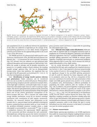
Recently, EPR spectroscopy has emerged as a powerful tool to study the structure and dynamics of biological
macromolecules such as proteins, protein aggregates, RNA and DNA. It is used in combination with molecular
modelling to study complex systems such as soluble proteins, membrane proteins and protein aggregates like
amyloid fibrils and oligomers.
https://www.ias.ac.in/article/fulltext/reso/020/11/1017-1032
moment. The otheris spinning around its own axis, which brings spin magnetic moment.
Like most spectroscopic techniques, EPR spectrometers measure the absorption of
electromagnetic radiation.
The EPR spectrum of a free radical is the simplest of all forms of spectroscopy. If an
external magnetic field is not present, the two electron spin states (spin up and spin down)
are degenerate. The degeneracy of the electron spin states characterized by the quantum
number, ms ¼ 1/2 is lifted by the use of a magnetic field. Transitions between the
electron spin levels are induced by radiation at the matching frequency. When a magnetic
field is induced, atoms with unpaired electrons spin either in the same direction (spin up)
or in the opposite direction (spin down) of the applied field. These two possible
alignments with different energies are no longer degenerate. The alignments are directly
proportional to the applied magnetic field strength. This is called the Zeeman effect. An
unpaired electron interacts with its environment, and the details of EPR spectra depend on
the nature of those interactions. The readings can provide information on structural and
dynamic information, even from the chemical or physical process, without influencing the
process itself. The energy associated with the transition is expressed in terms of the
applied magnetic field B, the electron spin g-factor g, and the constant mB, which is called
the Bohr magneton.
The EPR technique has been widely used to study the structure and function of biological
membranes.
Biological membranes play a vital role in the cell structure and function. Mass and
information transport through the membrane are the most important biological functions,
whereas the membranes divide the cell into several different compartments. Researches in
the past decades have shown that membranes consist of a laterally heterogeneous lipid
bilayer with a large number of embedded protein molecules. The bilayer is heterogeneous
either in the way of molecular assembly or in the way of the assembly of molecular
aggregates. The molecules and the super molecular aggregates thus interact with each
other by different interaction forces and exhibit a variety of characteristics in the transport.
The elucidation of the structure and function of the biological membrane has been
recognized as a formidable task. Despite its complexity, the EPR technique is considered
as one of the most important techniques, both experimentally and biologically.
Unlike biological membranes, the application of the EPR technique to investigate the
synthetic polymeric membranes is very rare and none can be found for ceramic
membranes. This is very surprising, considering the fact that the biomimetic membrane
such as aquaporin membrane currently occupies the center position in the development of
novel separation membranes.
It is attempted in this article to review the EPR applications for the study of synthetic
polymeric membranes. The fundamentals of the EPR technique that are outlined before
48 Chapter 3
72.
some examples ofEPR applications in the synthetic polymeric membranes are shown.
Then, the EPR works that have potential in the future investigation of separation
membranes are collected from the literature and the problems that should be addressed for
the wider applications of the EPR technique are shown.
2. Fundamentals of EPR
2.1 Principle of Electron Paramagnetic Resonance
Magnetic moment of the molecule is primarily contributed by unpaired electron (Fig. 3.1).
By increasing the external magnetic field, the gap between two energy states is widened
until it matches the energy of the microwaves, as represented by the double arrow in the
diagram above. At this point the unpaired electrons can move between their two spin
states. Since there are typically more electrons in the lower state, due to the
MaxwelleBoltzmann distribution, there is a net absorption of energy, and it is this
absorption that is monitored and converted into a spectrum (see Fig. 3.2). The upper
spectrum below is the simulated absorption for a system of free electrons in a varying
magnetic field. The lower spectrum is the first derivative of the absorption spectrum. The
latter is the most common way to record and publish EPR spectra.
If we are dealing with systems with a single spin like this example, then EPR would
always consist of just one line and would have little value as an investigative tool, but
several factors influence the effective value of g in different settings. Since the source of
an EPR spectrum is a change in an electron’s spin state, it might be thought that all EPR
spectra for a single electron spin would consist of one line. However, the interaction of
an unpaired electron, by way of its magnetic moment with nearby nuclear spins, results
in additional allowed energy states and, in turn, multilined spectra. In such cases, the
spacing between the EPR spectral lines indicates the degree of interaction between the
Figure 3.1
Energy levels for an electron spin (ms ¼ 1/2) in an applied magnetic field B0 [1].
Electron Paramagnetic Resonance (EPR) Spectroscopy 49
73.
unpaired electron andthe perturbing nuclei. The hyperfine coupling constant of a nucleus
is directly related to the spectral line spacing and, in the simplest cases, is essentially the
spacing.
Fundamentally EPR is similar to the more widely familiar method of nuclear magnetic
resonance (NMR) spectroscopy, with several important distinctions. Although both
spectroscopies deal with the interaction of electromagnetic radiation with magnetic
moments of particles, there are many differences between the two spectroscopies:
1. EPR focuses on the interactions between an external magnetic field and the unpaired
electrons of whatever system it is localized to, as opposed to the nuclei of individual
atoms.
2. The electromagnetic radiation used in NMR typically is confined to the radio frequency
range between 300 and 1000 MHz, whereas EPR is typically performed using micro-
waves in the 3e400 GHz range.
3. In EPR, the frequency is typically held constant, whereas the magnetic field strength is
varied. This is the reverse of how NMR experiments are typically performed, where the
magnetic field is held constant while the radio frequency is varied.
4. Due to the short relaxation times of electron spins in comparison to nuclei, EPR
experiments must often be performed at very low temperatures, often below 10K, and
sometimes as low as 2K. This typically requires the use of liquid helium as a coolant.
5. EPR spectroscopy is inherently roughly 1000 times more sensitive than NMR spectros-
copy due to the higher frequency of electromagnetic radiation used in EPR in
comparison to NMR.
Figure 3.2
Absorption of energy [1].
50 Chapter 3
74.
EPR permits observationof any substance having unpaired electrons. Some examples of
substances that exhibit this quality are as follows:
1. Atoms or ions having partially filled inner electron shells that are all of the transition
elements of the iron series, rare earth’s and platinum series.
2. Molecules having an odd number of electrons in their outer shells (e.g., NO or ClO2).
3. Molecules with an even number of electrons in their outer shells but with a resultant
magnetic moment (e.g., O2).
4. Free radicals, which are naturally or artificially produced.
5. Conduction electrons in metals and acceptors and donors in semiconductors.
6. Modified crystal structure and defects in crystals, e.g., color centers.
EPR study is affected by the degree of detail desired and by the type of problem
investigated. It is sensitive to the local environment.
2.2 Electron Spin and Magnetic Moment
As discussed earlier, an electron is a negatively charged particle with certain mass and has
mainly two kinds of movements. The first one is spinning around the nucleus, which
brings orbital magnetic moment, and the other is spinning around own axis, which brings
spin magnetic moment. Magnetic field of the molecule is primarily contributed by
unpaired electron’s spin magnetic moment, which is given by,
MS ¼
ffiffiffiffiffiffiffiffiffiffiffiffiffiffiffiffiffi
SðS þ 1Þ
p h
2p
(3.1)
MS is the total spin angular momentum, S is the spin quantum number, and h is Planck’s
constant. In the z direction, the component of the total spin angular moment can only
assume two values:
MSZ
¼ mS$
h
2p
(3.2)
the term ms has (2S þ 1) different values: þS, (S 1), (S 2),. S. For single unpaired
electron, only two possible values for ms are þ1/2 and 1/2.
The magnetic moment, me is directly proportional to the spin angular momentum and one
may therefore write
me ¼ gemBMS (3.3)
The appearance of negative sign is because the magnetic moment of electron is collinear
but antiparallel to the spin itself. The term (gemB) is the magnetogyric ratio. The factor ge
is known as the free electron g-factor with a value of 2.002 319 304 386 (one of the most
Electron Paramagnetic Resonance (EPR) Spectroscopy 51
75.
accurately known physicalconstants). The Bohr magneton, mB, is the magnetic moment
for one unit of quantum mechanical angular momentum:
mB ¼ ðehÞ=ð4pmeÞ (3.4)
where e is the electron charge, me is the electron mass.
This magnetic moment interacts with the applied magnetic field. The interaction between
the magnetic moment (me) and the field (B) is described by
E ¼ meB (3.5)
For single unpaired electron, there will be two possible energy states, this effect is called
Zeeman splitting.
Eþ1
2
¼
1
2
gmBB (3.6)
E1
2
¼
1
2
gmBB (3.7)
In the absence of external magnetic field, Eþ1/2 ¼ E1/2 ¼ 0.
In the presence of external magnetic field, as illustrated in Fig. 3.1, with the absorption of
radiation, the difference between the two energy states can be written as
DE ¼ hv ¼ gmBB (3.8)
With the intensity of the applied magnetic field increasing, the energy difference between
the energy levels widens until it matches with the microwave radiation and results in
absorption of photons.
2.3 Hyperfine Coupling
Since the source of an EPR spectrum is a change in an electron’s spin state, it might be
thought that all EPR spectra for a single electron spin would consist of one line. However,
the interaction of an unpaired electron, by way of its magnetic moment, with nearby
nuclear spins, results in additional allowed energy states and, in turn, multilined spectra. In
such cases, the spacing between the EPR spectral lines indicates the degree of interaction
between the unpaired electron and the perturbing nuclei. The hyperfine coupling constant
of a nucleus is directly related to the spectral line spacing and, in the simplest cases, is
essentially the spacing itself.
2.4 Block Diagram of EPR Spectrometer
Fig. 3.3 shows a block diagram for a typical EPR spectrometer. The radiation source
usually used is called a klystron. Klystrons are vacuum tubes known to be stable
52 Chapter 3
76.
high-power microwave sources,which have low-noise characteristics and thus give high
sensitivity. A majority of EPR spectrometers operate at approximately 9.5 GHz, which
corresponds to about 32 mm. The radiation may be incident on the sample continuously
[i.e., continuous wave (cw)] or pulsed. The sample is placed in a resonant cavity, which
admits microwaves through an iris. The cavity is located in the middle of an
electromagnet and helps to amplify the weak signals from the sample. Numerous types
of solid-state diodes are sensitive to microwave energy and absorption lines then can be
detected when the separation of the energy levels is equal or very close to the
frequency of the incident microwave photons. In practice, most of the external
components, such as the source and detector, are contained within a microwave bridge
control. Additionally, other components, such as an attenuator, field modulator, and
amplifier, are also included to enhance the performance of the instrument.
2.5 Spin-Labeling Method
Most chemical and biological samples of interest for EPR spectroscopy lack an inherent
stable unpaired electron, the majority of EPR methods rely on the usage of spin-labeling
reagents. The radical so introduced is often called a spin label or a spin probe. It is
invariably a nitroxide radical, which exhibits a three-line hyperfine structure whose peak
shape, splitting, etc., depend on the radical’s environments. The nitroxide label is a monitor
of motion. The shape of the EPR signal depends also on the orientation of the magnetic
field relative to the axis of the radical. Thus, the spin label method is useful to study the
environment of radical, which is the structure of the polymer at a molecular level.
Figure 3.3
Block diagram for a typical electron paramagnetic resonance spectrometer [2].
Electron Paramagnetic Resonance (EPR) Spectroscopy 53
77.
Commonly, nitroxides suchas derivatives of TEMPO (2,2,6,6-tetramethyl-1-
piperidinyloxy) are used as they offer high stability of the unpaired electron and
exceptional EPR sensitivity combined with facile and versatile moieties for binding to the
sample through chemical reactions itself. Fig. 3.4 shows the EPR spectra of TEMPO
solution in water (0.02 wt%). The spectra consist of three symmetric peaks since the NO*
radical of TEMPO (or with 5-, 12-, and 16-doxylstearic acid derivatives) is freely mobile
in the solution. The spectra are isotropic (symmetric) and the value of Hamiltonian
parameter, the factor ge is known as the free electron g-factor with a value of 2.002 319
304 386 (one of the most accurately known physical constants) and ǀAǀ (distance between
two peaks) is 17 G. All three peaks are almost equal in height and symmetric.
Interactions of an unpaired electron with its environment influence the shape of an EPR
spectral line. The shape of curves and other properties of the EPR spectra gives the clue
for analysis.
3. EPR Applications for the Synthetic Polymeric Membranes
3.1 EPR Applications at the University of Ottawa
Khulbe and Matsuura [4] wrote a review in which they discussed the characterization of
synthetic membranes by EPR.
Figure 3.4
Electron paramagnetic resonance spectra of 2,2,6,6-tetramethyl-1-piperidinyloxy solution in water
(0.02 wt%) [3].
54 Chapter 3
78.
The radicals weredetected in the polymeric material from which membranes are
fabricated and the number of radicals depended on the conditions in which the membranes
were fabricated and the environment to which the membranes were exposed. Polymers
themselves contain paramagnetic free radicals. It is possible that these radicals may take
part in the transportation of gases through the membrane. It is observed that these radicals
are affected reversibly with gases (CO2 and CH4). Khulbe et al. [5] reported that
polyphenylene oxide (PPO) radicals are present in PPO powder, and the membranes
prepared from PPO contain free radicals that are affected by the conditions of the
environment. It was reported that the number of spins/g in membranes is higher than in
the PPO powder and it also depends on the characteristics of solvents used for membrane
preparation. Generally, the number of spins/g in vacuum is less than in the air. However,
no definite conclusion could be drawn due to small quantity of spins (1014
spins/g). It was
noticed that in the presence of N2 the number of spins/g (concentration) was more than
that in the presence of O2. On the contrary, the number of spins/g was higher in the
presence of CH4 than CO2. The permeation rates through the membrane of CO2 and O2
are usually higher than CH4 and N2, respectively. This type of behavior also was observed
with sulfonated and brominated PPO membranes [4].
Incorporation of the spin label TEMPO was also attempted by Khulbe et al. [6]. Dense
homogeneous PPO membranes were prepared by casting a solution, which consisted of
PPO, TEMPO (spin probe), and 1,1,2-trichloroethylene solvent. The solvent was
evaporated at 22, 4, and 10C. Membranes were subjected to EPR spectroscopic study as
well as to the permeability measurement of various gases, including O2, N2, CO2, and
CH4. It was observed that the intensity of the spin probe decreased with the decrease of
temperature used for the preparation of the membrane. The intensity of the spin probe was
almost at zero level for the membrane prepared at 10C in comparison with the EPR
signal intensity of the other two membranes prepared at higher temperatures. It could be
due to high crystallinity state in the membrane prepared at 10C or some level of
molecular ordering. Authors concluded that
1. The intensity of the spin probe in the PPO membrane depends on the temperature of
solvent evaporation during dense membrane preparation.
2. The morphology of the surface on the membrane depends on the temperature used for
the preparation of the membrane.
3. Generally, the permeation rate of gases (especially with CO2 and CH4) increases with
the decrease in the temperature used for the preparation of membrane. It could be
possible that Langmuir sites are most favorable for the CH4 and N2 permeation in PPO
membrane. It could be possible that Henry sites are good for selectivity.
Gumi et al. [7] studied activated composite membranes by EPR and reported that EPR is a
useful tool for the characterization of activated composite membranes.
Electron Paramagnetic Resonance (EPR) Spectroscopy 55
79.
Another example ofthe incorporation of spin label is the work by Khulbe et al. [3]
who prepared dense membranes from poly(phenylene oxide) (PPO) by blending spin
probes (TEMPO, 5-, 12-, and 16-doxylstearic acid) in the casting solution. It was
noticed that the shape and size of the probe influence the EPR spectra of the NO*
radical in the PPO membrane. Unexpectedly, from the shape of the EPR signal it was
noticed that the NO*
radical of TEMPO in PPO membrane was more mobile than in
water media. However, the motion of the NO*
radical of 16-doxylstearic acid was
higher than that of NO*
radical of 5- and 12-doxylstearic acid when the radicals were
in the PPO membrane. This could be due to the inductive effect from COOH group.
The Hamiltonian parameters of the EPR signal indicated that all the probes were not
randomly distributed in the PPO membrane, but some probes were distributed in the
polymer in orderly fashion.
Khulbe et al. [8] studied the structure of the skin layer of asymmetric cellulose acetate
(CA) RO membranes with TEMPO probe. It was observed that the mobility of TEMPO in
the asymmetric membrane shrunk at 90C was the same as TEMPO in a dense
homogeneous membrane prepared from the same casting solution. Authors reported the
following conclusions
1. The pore sizes of the asymmetric membranes are larger when they were shrunk at lower
temperatures
2. The space in the polymer network (the origin of the network pore) in the dense film
was smaller when no swelling agent is added to the casting solution
3. The space in the polymer network in the dense film was smaller when the membrane
was dry
In another study, Khulbe et al. [9] used EPRspectroscopy as a method to study membrane
fouling during ultrafiltration (UF). Bovine serum albumin (BSA) and polyethylene oxide,
with and without TEMPO (spin probe), solutions in water were used as the feed in the UF
experiments. Asymmetric membranes were prepared by phase inversion technique using
casting solutions of polyethersulfone (PES) in n-methyl pyrrolidone. Polyvinyl pyrrolidone
was added as a nonsolvent additive. The following conclusions were reported.
1. Deposition of BSA on the surface and inside the pore during UF is in a specific orienta-
tion (manner). However, the orientation of BSA molecule on the surface is different
from that of the BSA molecule inside the pore.
2. The packing density of BSA molecules inside the pore depends on the particular pore
size and feed pressure. At higher feed pressure, the denser packing moves toward
smaller pore size.
3. Fouling depends on the structure of solute.
EPR spectroscopy technique was also used to study CA membranes for reverse osmosis
(RO) and PES membranes for UF [10]. TEMPO was used as a spin probe that was
56 Chapter 3
80.
brought into themembranes by immersing the membranes into solutions involving
TEMPO, or by blending TEMPO into membrane casting solutions. The following
conclusions were reported:
1. EPR technique can be used to study the structure and the transport of RO and UF
membranes.
2. Water may flow through the pores of PES membranes. The sizes of pores are those of
UF membranes. Unlike CA, the polymer matrix of PES membrane is a little swollen or
not at all swollen by water and continuous channels through which water flows cannot
be formed. In CA, spaces in water swollen polymer matrix were the primary provider
of continuous flow channels that contribute to the separation of salt and small organic
molecules. In the absence of such water channels, PES membranes cannot act as RO
membranes.
Khulbe et al. [11] reported the EPR study on the structure and transport of asymmetric
aromatic polyamide membranes. TEMPO was used as a spin probe that was brought into
the membrane by (a) immersion of the membranes in aqueous TEMPO solutions, (b) RO
experiments with feed solutions involving TEMPO, or (c) blending TEMPO in casting
solutions. The membranes were tested for the separation of sodium chloride and TEMPO
from water by RO. It was concluded that aromatic polyamide membranes contain water
channels in the polymer matrix like CA membranes. A comparison was made with other
RO membranes (CA) and UF membranes (PES). It was suggested that the EPR
technique can be used to study the structure of UF and RO membranes. The presence of
water channels in the polymer matrix seems indispensable for the RO membrane.
3.2 Applications of EPR to Study Fouling of RO and UF Membranes
Membrane fouling and aging were studied by the other groups using EPR technique.
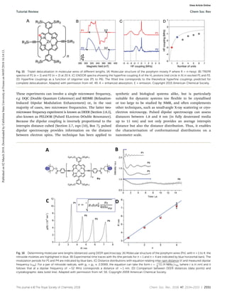
Oppenheim et al. [12] spin-labeled hen egg lysozyme (HEL) with 3-maleimido-proxy at
two positions of macromolecule. HEL solution was ultrafiltered in a cross-flow UF
apparatus for 2 h using polysulfone UF membrane of molecular weight cutoff (MWCO) ¼
10 kDa. Then, spin-labeled HEL in saline buffer solution and on the UF membrane were
subjected to EPR analysis. Figs. 3.5 and 3.6 show the EPR signals obtained from HEL in
the buffer solution and HEL in the UF membrane, respectively. The peaks indicated in
Fig. 3.6 by arrows were ascribed by the authors to the spinespin interaction between two
spin labels of HELs confined in narrow pore channels. When HEL was ultrafiltered by UF
membrane of MWCO ¼ 30 kDa, the EPR signal was similar to that of HEL in the buffer
solution, indicating the pores of the latter membrane (MWCO ¼ 30 kDa) were not blocked
by HELs.
RO and UF membranes are often cleaned chemically by contacting the membranes with
hypochlorite solution. It has long been suggested that degradation of polymer takes place
Electron Paramagnetic Resonance (EPR) Spectroscopy 57
81.
during the membranecleaning due to radical formation [13]. To confirm this hypothesis
Oliveira et al. studied, using EPR technique, the aging of polyamide thin film composite
membrane during the chemical cleaning by hypochlorite solution changing the
hypochlorite concentration as well as pH [14].
Figure 3.5
Electron paramagnetic resonance signal from the hen egg lysozyme in buffer solution [12].
Figure 3.6
Electron paramagnetic resonance signal from the hen egg lysozyme in the UF membrane
(MWCO 10 kDa) pore [12].
58 Chapter 3
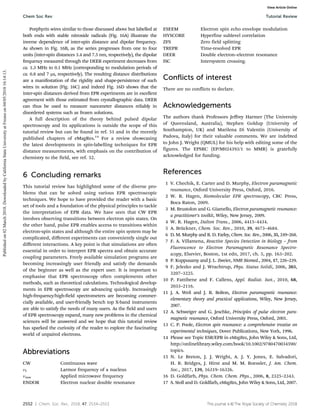
82.
Dow Filmtech NF270 membrane was immersed in bleach solution (NaClO3) before the
membrane was dried and transferred into a quartz tube for EPR observation. The intensity
of the EPR signal has increased with an increase of bleach concentration as shown in
Fig. 3.7, whereas the radical formation was suppressed by increasing pH (Fig. 3.8).
Unfortunately, the radical species could not be identified due to the absence of the
hyperfine structure.
They have also studied the effect of the membrane exposure to the sunlight on the
radical formation and the radical formation during the ultraviolet (UV) membrane
surface grafting and confirmed that the membrane degradation occurred under an
excessive UV irradiation.
4. Other Examples of EPR Applications
4.1 Aging of Proton Exchange Membranes
The degradation of proton exchange membranes (PEMs) is an important subject in the fuel
cell application. As a typical PEM Nafion was chosen and its degradation mechanism was
studied by EPR when Nafion was neutralized by Cu(II), Fe(II), and Fe(III) ions [15].
When Nafion was neutralized by FeSO4 and irradiated by UV, the signal from ROCF2CF2$
radical was detected and its intensity increased with the UV irradiation time (Fig. 3.9).
Remarkably, the signal was also observed even before the UV irradiation, indicating
radical formation in the presence of Fe(II) without UV irradiation. At the same time the
formation of Fe(III) was detected.
Figure 3.7
Electron paramagnetic resonance spectra taken after the membrane was immersed in bleach
solution of (a) 80, (b) 50, and (c) 20 v/v% [14].
Electron Paramagnetic Resonance (EPR) Spectroscopy 59
83.
Figure 3.8
Electron paramagneticresonance spectra after the membrane was immersed in 50 v/v% bleach
solution at (a) pH ¼ 8 and (b) pH ¼ 9 [14].
Figure 3.9
Electron paramagnetic resonance signal for ROCF2CF2$ radical when neutralized by Fe(II) [15].
60 Chapter 3
84.
Thus, the radicalformation and polymer degradation are possible in the presence of metal
ions such and Cu(II), Fe(II), and Fe(III) even without UV irradiation.
4.2 Study of Carbon Nanotubes
Much attention has been paid to carbon nanotubes (CNTs) to apply them for separation
membranes due to their extraordinarily high permeability for water and gas. Many
attempts have also been made to incorporate them in the mixed matrix membranes
(MMMs) [16]. The study of CNTs by EPR was conducted even before the
announcement of the unusual permeation characteristics of CNTs by Hinds et al. [17].
Multiwalled CNTs were embedded in styrene-polyisoprene-polystyrene (SIS) block
copolymer and its EPR spectra were recorded [18]. The resonance spectrum of SIS-CNTs
composite is featured by a strong and symmetric peak at g ¼ 2.06 and the resonance line
width of 102
G, which was ascribed to the strongly interacting localized and itinerant
electrons, in the so-called bottleneck state.
The double integral of the resonance line called S is proportional to the susceptibility.
When S is plotted versus temperature (Fig. 3.10), S depends only weakly on
temperature when the CNT content in the composite is low, but S depends strongly on
temperature when the CNT content is high. Since susceptibility S of localized electron
is temperature dependent, whereas S of delocalized electron is temperature independent,
Fig. 3.10 means that the amount of localized electron is very small when the CNT
content is low. These localized electrons were most likely those of Feþ3
ions in the
residual catalyst of CNT synthesis. As the CNT loading increases, the amount of
Figure 3.10
Temperature dependence of S [18].
Electron Paramagnetic Resonance (EPR) Spectroscopy 61
85.
localized electrons (paramagneticdefects) increases and so does the temperature
dependency. This means these paramagnetic defects are localized either within CNTs
themselves or at the CNTsepolymer interface.
Another study on CNTs was done by Rao et al. [19].
Double walled carbon nanotubes of 0.45 nm average diameter were embedded in VP 15
molecular sieve (zeolite) nanochannels and subjected to EPR at temperatures 4.2, 20, 40,
60, and 75K. From Fig. 3.11, for all temperatures a symmetric EPR signal is observed at
gc z 2.0028 with a corresponding density z1019
g1
.
Generally, for single walled carbon nanotubes (SWCNTs) and MWCNTs of much larger
diameter (more than 1 nm) different types of EPR signals are observed, i.e., (1) signal
centered at gc ¼ 2.0 coming from the residual metal catalytic particles, (2) gc ¼ 2.07
coming from the conduction electron spin resonance, and (3) gc ¼ 2.00 coming from
localized electron spins. Therefore, Fig. 3.11 excludes the possibility of the presence of
conduction electrons. The electrons are localized in the defect on the CNTs.
Figure 3.11
Electron paramagnetic resonance signal of carbon nanotubes embedded in zeolite at different
temperatures [19].
62 Chapter 3
86.
4.3 Metal OrganicFrameworks
Much attention is also paid to metal organic frameworks (MOFs) due to its unique
structures that allow strong adsorption of gaseous molecules [20]. They are also embedded
in polymeric membrane to form MMMs for gas and liquid separation [21].
MOF expands in their crystalline structure when guest molecules are adsorbed in it,
whereas it shrinks when the molecules are desorbed, a phenomena known as
“breathing.” It was confirmed by EPR that similar structural change takes place when
temperature changes from high (HT) to low (LT) and vice versa. Cr(III)-doped
aluminum-based MIL-53 was synthesized where the main metal ion is Al (99%),
whereas the rest of 1% is Cr. The sample was further calcinated and evacuated to
remove water and residual organic acid and it was called MIL-53(Al/Cr)deh, where deh
means dehydration.
The Q-band EPR spectra of MIL-53(Al/Cr)deh taken at different temperatures are shown
in Fig. 3.12.
At 295K (Fig. 3.12(a,b)), three singularities (q ¼ 0 degree, 42 degree, and 90 degree) of
the central MS ¼ 1/2 4 ½ transition appear between 1170 and 1320 mT. Furthermore,
two single q ¼ 90 degree edge singularities of the MS ¼ 3/2 4 ½ transitions are
observed at 940 and 1540 mT without splitting, indicating an axially symmetric tensor
(E z 0). Then, the ratio of spin Hamiltonian parameters E/D becomes nearly equal to
Figure 3.12
Electron paramagnetic resonance spectra of MIL-53(Al/Cr)deh at (a) experimental, (b) simulated
at 295K, (c) experimental, and (d) simulated at 5K [21].
Electron Paramagnetic Resonance (EPR) Spectroscopy 63
87.
zero, hence thesesignals are assigned to CrO4(OH)2 octahedral (Fig. 3.13(a)) in the HT
phase of MIL-53(Al/Cr)deh.
On the other hand, at a lower temperature of 5K, the Q-band spectrum transformed to
rhombic nature (Fig. 3.12(c,d)) and the signals at 940 and 1540 mT disappeared, which
means the ratio of spin Hamiltonian parameters E/D is no longer zero (by simulation E/D
ratio was found to be 0.236), suggesting the lowering in the symmetry of CrO4(OH)2
octahedrons (see Fig. 3.13(b)).
It was further proposed that high to low temperature transition occurs at temperatures
between 150 and 60K, whereas the transformation from low to high transition occurs at
the temperatures between 330 and 375K, indicating the large thermal hysteresis. As
well about 20% of the material does not undergo the transition high to low
temperature.
4.4 State of Interfacial Water
Two polypeptides, 26-residue polypeptide (n3) and 14-mer long proline model peptide
(PPm3), were spin labeled and dissolved in vitrified solvent (concentrated aqueous
sucrose or glycerol solution) or confined in two mesoporous silica materials, SBA15a
Figure 3.13
Schematic presentation of MIL-53(Al/Cr)deh structure, (a) 295K, (b) 5K [21].
64 Chapter 3
88.
and SBA15b, withpore diameters of 7.6 and 6.1 nm, respectively. Then, they were
subjected to several EPR studies including double electron resonance, electron spin
echo, and electron spin echo envelope modulation (ESEEM). As well, H2O was
sometimes changed to D2O [22]. The parameter p(D2O) measured by ESEEM shows
the accessibility of water, especially D2O, within the van der Waals contact distance of
c. 0.35 nm from the spin label.
As shown in Table 3.1, p parameter does not change in the vitrified solvent or in the pore
of SBA 15a and SBA 15b. Only when the peptide PPm3 was in the vitrified solvent
containing 40% glycerol, the accessibility was nearly doubled.
On the other hand, the parameter Cex, which indicates the density of water (D2O in this
case) within the range of 2 nm of the spin label is remarkably different, depending on
the confinement in the nanopore. The values for both n3 and PPm3 are in the order of
SBA 15b SBA 15a vitrified solvent and remarkably high when the polypeptides are
confined in SBA 15b with the nanopores of the smaller diameter. Thus, this result
confirms that there is density profile in the vicinity of the spin-labeled polypeptide,
indicating the presence of special water near polypeptides that represent proteins,
so-called “biological surface water.” The importance of such water for sustaining
“life” is well recognized.
The presence of special water in RO membrane, most likely in the membrane pore, has
long been recognized by differential scanning calorimetric (DSC) experiments [23]. Thus,
EPR can possibly be a powerful tool to sense the presence of special interfacial water in
the membrane pore.
5. Conclusions
It was shown that the EPR technique is a powerful tool to study the synthetic polymeric
membranes by showing:
1) Radicals are present in the synthetic polymeric membrane.
Table 3.1: p Parameter and density (Cex) profile in the vicinity of spin-labeled polypeptide.
p Cex (n/m3
)
26-residue polypeptide (n3) in
SBA 15a
0.185 24.2
n3 in SBA 15b 0.156 42.3
n3 in 40% sucrose solution 0.142 12.8
14-mer long proline model
peptide (PPm3) in SBA 15a
0.215 28.6
PPm3 in SBA 15b 0.132 60.9
PPm3 in 40% glycerol solution 0.479 23.0
Electron Paramagnetic Resonance (EPR) Spectroscopy 65
89.
1.1) The concentrationof radicals is different depending on the conditions by which
membranes are fabricated. The macromolecular radicals in the membrane may
lead to the degradation of polymer by radical reactions.
1.2) The radical concentration increases during the chemical cleaning of the mem-
brane, leading to polymer degradation. The radical concentration also increases
by exposure to sunlight and during the surface modification by UV grafting.
2) The spin-labeling technique is a powerful tool to characterize the membrane
morphology. In particular,
2.1) The order in the macromolecular alignment in the membrane can be detected at
the molecular level, which might affect the membrane selectivity in gas
separation.
2.2) The difference in the nature of the pores in RO and UF membranes can be
identified. Water passes through the swollen intersegmental space (network
pores) in the skin layer of the CA RO membrane, whereas in the PES UF
membrane water flows through pores formed between the polymer aggregates
(aggregate pores).
2.3) The network pores of the CA membranes shrink when the membrane is annealed.
2.4) EPR technique confirms that membrane fouling takes place by protein molecules
that are densely packed in the membrane pores.
It was shown by some other examples that
1) Radicals were found in the Nafion PEMs when its sulfonic group was partially
neutralized by Cu or Fe ions, causing the degradation of the PEMs.
2) It was found that the electron was highly localized in the CNT itself, in the space
between CNT and polymer matrix, or in the defect of CNTs.
3) Hysteresis was observed between the expansion of MOF at the HT and shrinkage at the
LT, which resembles the breathing of MOF that occurs by adsorption and desorption of
guest molecules.
4) The density profile was detected near protein molecules that are confined in nano-
channels. This proves the presence of the interfacial water at the protein/water
interface.
It should also be noted that the EPR applications for the synthetic polymeric membranes,
although they can give some insights into the membrane structure and performance, all of
the currently available works lack precise analysis of the hyperfine structures of the EPR
signals.
On the other hand, in the other works, the hyperfine structures of EPR signals were
analyzed more rigorously, giving details of the EPR signal sources. Unfortunately,
however, it is very difficult to understand how the EPR parameters can be interpreted due
to the complexity of the EPR theory.
66 Chapter 3
90.
As well, EPRtechnique has the following drawbacks compared to the other
characterization techniques.
1) It is impossible to obtain two-dimensional (2D) or three-dimensional (3D) images of
the membrane surface (and the cross-section) unlike scanning electron microscope,
transmission electron microscope, and atomic force microscope.
2) Currently, it is impossible to investigate the surface of the membrane separately from
the bulk, unlike FTIR-ATR, XPS, EDX, and contact angle measurement.
3) Hence, the data are affected by the bulk structures under the top surface layer that
governs the performance of the asymmetric membrane, similar to XRD, DSC, TGA,
and measurement of mechanical strength.
Thus, the complication involved in the theoretical interpretation of EPR, absence of 2D
and 3D images taken by the EPR technique and difficulty in the surface observation is
now hampering the wider usage of the EPR technique to investigate the synthetic
polymeric membrane despite its enormous potential to reveal the details of the membrane
structure.
References
[1] UC Davis ChemWiki, http://chemwiki.ucdavis.edu/Physical_Chemistry/Spectroscopy/Magnetic_
Resonance_Spectroscopies/Electron_Paramagnetic_Resonance/EPR%3A_Theory.
[2] What is EPR spectroscopy?: University of Texas at Austin. http://epr.cm.utexas.edu/WhatIsEPR.html.
[3] Khulbe KC, Hamad F, Feng C, Matsuura T, Gumi T, Palet C. ESR spectra of spin probe in PPO
membrane. Polymer 2003;44:695e701.
[4] Khulbe KC, Matsuura T. Characterization of synthetic membranes by Raman spectroscopy, electron spin
resonance, and atomic force microscopy; a review. Polymer 2000;41:1917e35.
[5] Khulbe KC, Chowdhury G, Matsuura T, Lamarche G. Characterization of PPO [poly(phenylene oxide) ]
powder and membranes from it by ESR technique. J Membr Sci 1997;123:9e15.
[6] Khulbe KC, Chowdhury G, Kruczek B, Vujosevic R, Matsuura T, Lamarche G. Characterization of the
PPO dense membrane prepared at different temperatures by ESR, atomic force microscope and gas
permeation. J Membr Sci 1997;126:115e22.
[7] Gumi T, Valiente M, Khulbe KC, Palet C, Matsuura T. Characterization of activated composite
membranes by solute transport, contact angle measurement, AFM and ESR. J Membr Sci
2003;212:123e34.
[8] Khulbe KC, Matsuura T, Lamarche G, Lamarche A-M, Choi C, Noh SH. Study of the structure of
asymmetric cellulose acetate membranes for reverse osmosis using electron spin resonance (ESR) method.
Polymer 2001;42:6479e84.
[9] Khulbe KC, Matsuura T, Singh S, Lamarche G, Noh SH. Study on fouling of ultrafiltration membrane by
electron spin resonance. J Membr Sci 2000;167:263e73.
[10] Khulbe KC, Matsuura T, Feng SCY. Study on cellulose acetate membranes for reverse osmosis and
polyethersulfone membranes for ultrafiltration by electron spin resonance technique. Desalination
2002;148:329e32.
[11] Khulbe KC, Feng C, Matsuura T, Lamarche G, Lamarche A-M. Study of the structure of asymmetric
polyamide membranes for reverse osmosis using the electron spin resonance (ESR) method. Desalination
2003;154:1e8.
Electron Paramagnetic Resonance (EPR) Spectroscopy 67
91.
[12] Oppenheim SF,Buettner GR, Dordick JS, Rodgers VGJ. Applying electron paramagnetic resonance
spectroscopy to the study of fouling in protein ultrafiltration. J Membr Sci 1994;96:289e97.
[13] Kwon Y-N, Leckie JO. Hypochlorite degradation of crosslinked polyamide membranes I. Changes in
chemical/morphological properties. J Membr Sci 2006;283:21e6.
[14] Oliveira FRP, Matos CT, Moura JJG, Portugal CAM, Crespo JG. Study of membrane ageing and grafting
mechanisms using electron paramagnetic resonance. Desalination Water Treat 2011;27:150e8.
[15] Kadirov MK, Bosnjakovic A, Schlick S. Membrane-derived fluorinated radicals detected by electron spin
resonance in UV-irradiated nafion and Dow ionomers: efffect of counterions and H2O2. J Phys Chem B
2005;109:7664e70.
[16] Yang HY, Han ZJ, Yu SF, Pey KL, Osrikov K, Karnik R. Carbon nanotube membranes with ultrahigh
specific adsorption capacity for water desalination and purification. Nat Commun 2013;4. http://dx.doi.org/
10.1038/ncomms3220. Article number: 2220.
[17] Hinds BJ, Chopra N, Rantell T, Andrews R, Gavalas V, Bachas LG. Aligned multiwalled carbon nanotube
membranes. Science 2004;303:62e5.
[18] Chipara M, Zaleski JM, Hui D, Du C, Pan N. Electron spin resonance on carbon nanotubes-polymer
composites. J Polym Sci Part B 2005;43:3406e12.
[19] Rao SS, Stesmans A, Noyen JV, Jacobs P, Sels B. Electron spin resonance investigation of ultra-small
double walled carbon nanotubes embedded in zeolite nanochannels. J Phys Condens Matter
2011;23:455801. 6 pp.
[20] Hartmann M, Kunz S, Himsl D, Tangermann O. Adsorptive separation of isobutene and isobutane on
Cu3(BTC)2. Langmuir 2008;24:8634e42.
[21] Mendt M, Jee B, Stock N, Ahnfeldt T, Hartmann M, Himsl D, Pöppl A. Structural phase transitions and
thermal hysteresis in the metalorganic framework compound MIL-53 as studied by electron spin
resonance spectroscopy. J Phys Chem C 2010;114:19443e51.
[22] Lai Y-C, Chen Y-F, Chiang Y-W. ESR study of interfacial hydration layers of polypeptides in water-filled
nanochannels and in vitrified bulk solvents. PLoS One 2013;8:e68264. p. 130.
[23] Taniguchi Y, Horigome S. The states of water in cellulose acetate membranes. J Appl Polym Sci
1975;19:2743e8.
68 Chapter 3

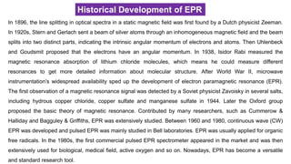
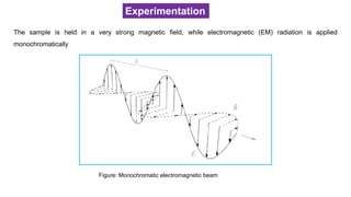
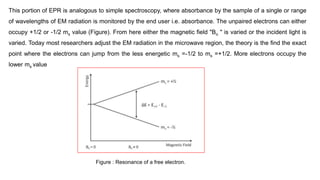
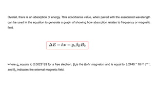
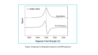
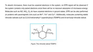
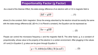
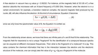
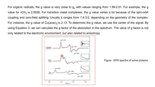
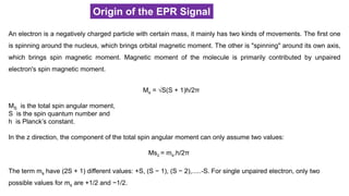
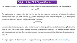
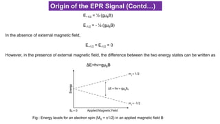
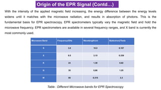
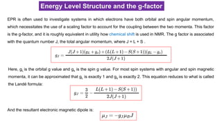
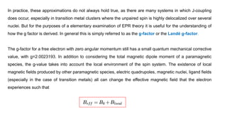
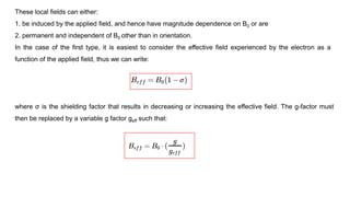
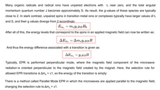
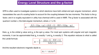
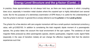
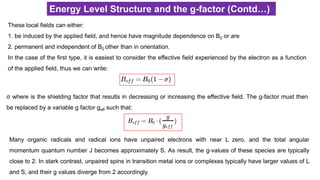
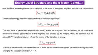
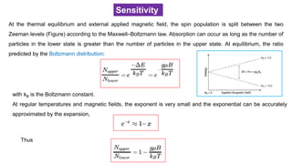
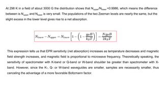
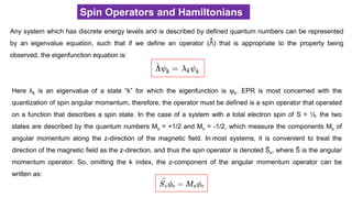
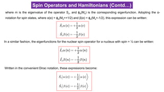
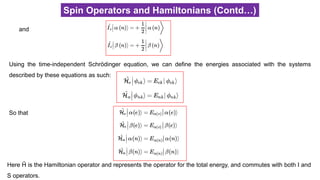
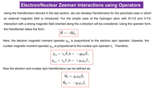
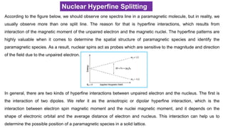
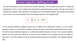
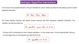
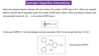
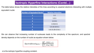
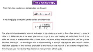
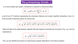
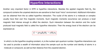
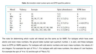
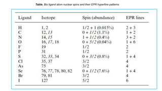
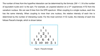
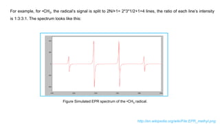
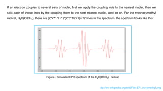
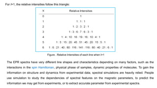
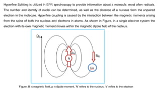
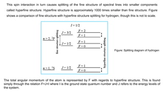
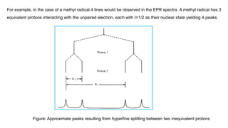
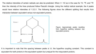
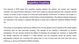
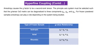
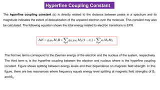
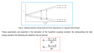
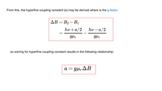
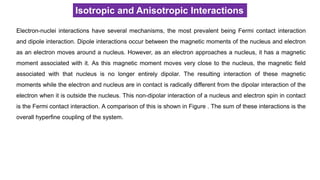
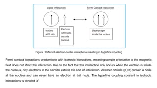
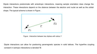
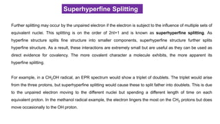
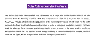
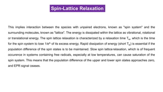
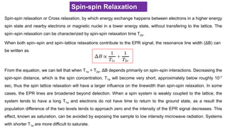
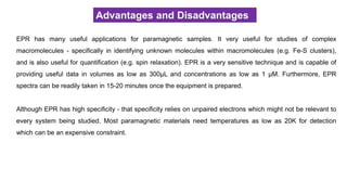
![Biological Applications
EPR is a very useful tool to study proteins with metal clusters, as proteins are usually in low concentration and
volume. Just the ability of EPR to probe a metal site in an enzyme reveals information. For example, in [NiFe]
hydrogenase there are many steps in the catalytic cycle where an iron atom is EPR silent and a nickel atom
switches between EPR active and silent depending on the catalytic state. This, coupled with coordination
information from the crystal structure, is strong evidence that the EPR silent iron must be low spin Fe(II) and the
nickel cycles between Ni(I) and Ni(II) in the different catalytic states.
Also, it is very popular to spin label sites in a protein for exploration with EPR. Spin labeling usually takes advantage
of the reactivity of protein thiol groups from cysteines. The most commonly used spin label is a nitroxyl radical
bound to a larger heterocyclic ring. In principle this allows previously EPR silent regions to be explored. By using
complex pulsed EPR techniques, such as double electron electron resonance, the distances between spin labels (or
natural paramagnetic sites) can be determined - this is especially useful when crystallographic structures are
unavailable.
Recently, EPR spectroscopy has emerged as a powerful tool to study the structure and dynamics of biological
macromolecules such as proteins, protein aggregates, RNA and DNA. It is used in combination with molecular
modelling to study complex systems such as soluble proteins, membrane proteins and protein aggregates like
amyloid fibrils and oligomers.
https://www.ias.ac.in/article/fulltext/reso/020/11/1017-1032](https://image.slidesharecdn.com/epr-spectroscopy-250607060036-53afcfd1/85/EPR-Spectroscopy-pdf-spectreral-techicque-68-320.jpg)

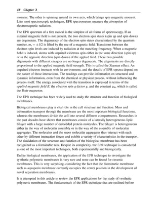
![some examples of EPR applications in the synthetic polymeric membranes are shown.
Then, the EPR works that have potential in the future investigation of separation
membranes are collected from the literature and the problems that should be addressed for
the wider applications of the EPR technique are shown.
2. Fundamentals of EPR
2.1 Principle of Electron Paramagnetic Resonance
Magnetic moment of the molecule is primarily contributed by unpaired electron (Fig. 3.1).
By increasing the external magnetic field, the gap between two energy states is widened
until it matches the energy of the microwaves, as represented by the double arrow in the
diagram above. At this point the unpaired electrons can move between their two spin
states. Since there are typically more electrons in the lower state, due to the
MaxwelleBoltzmann distribution, there is a net absorption of energy, and it is this
absorption that is monitored and converted into a spectrum (see Fig. 3.2). The upper
spectrum below is the simulated absorption for a system of free electrons in a varying
magnetic field. The lower spectrum is the first derivative of the absorption spectrum. The
latter is the most common way to record and publish EPR spectra.
If we are dealing with systems with a single spin like this example, then EPR would
always consist of just one line and would have little value as an investigative tool, but
several factors influence the effective value of g in different settings. Since the source of
an EPR spectrum is a change in an electron’s spin state, it might be thought that all EPR
spectra for a single electron spin would consist of one line. However, the interaction of
an unpaired electron, by way of its magnetic moment with nearby nuclear spins, results
in additional allowed energy states and, in turn, multilined spectra. In such cases, the
spacing between the EPR spectral lines indicates the degree of interaction between the
Figure 3.1
Energy levels for an electron spin (ms ¼ 1/2) in an applied magnetic field B0 [1].
Electron Paramagnetic Resonance (EPR) Spectroscopy 49](https://image.slidesharecdn.com/epr-spectroscopy-250607060036-53afcfd1/85/EPR-Spectroscopy-pdf-spectreral-techicque-72-320.jpg)
![unpaired electron and the perturbing nuclei. The hyperfine coupling constant of a nucleus
is directly related to the spectral line spacing and, in the simplest cases, is essentially the
spacing.
Fundamentally EPR is similar to the more widely familiar method of nuclear magnetic
resonance (NMR) spectroscopy, with several important distinctions. Although both
spectroscopies deal with the interaction of electromagnetic radiation with magnetic
moments of particles, there are many differences between the two spectroscopies:
1. EPR focuses on the interactions between an external magnetic field and the unpaired
electrons of whatever system it is localized to, as opposed to the nuclei of individual
atoms.
2. The electromagnetic radiation used in NMR typically is confined to the radio frequency
range between 300 and 1000 MHz, whereas EPR is typically performed using micro-
waves in the 3e400 GHz range.
3. In EPR, the frequency is typically held constant, whereas the magnetic field strength is
varied. This is the reverse of how NMR experiments are typically performed, where the
magnetic field is held constant while the radio frequency is varied.
4. Due to the short relaxation times of electron spins in comparison to nuclei, EPR
experiments must often be performed at very low temperatures, often below 10K, and
sometimes as low as 2K. This typically requires the use of liquid helium as a coolant.
5. EPR spectroscopy is inherently roughly 1000 times more sensitive than NMR spectros-
copy due to the higher frequency of electromagnetic radiation used in EPR in
comparison to NMR.
Figure 3.2
Absorption of energy [1].
50 Chapter 3](https://image.slidesharecdn.com/epr-spectroscopy-250607060036-53afcfd1/85/EPR-Spectroscopy-pdf-spectreral-techicque-73-320.jpg)
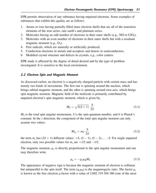
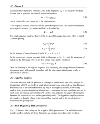
![high-power microwave sources, which have low-noise characteristics and thus give high
sensitivity. A majority of EPR spectrometers operate at approximately 9.5 GHz, which
corresponds to about 32 mm. The radiation may be incident on the sample continuously
[i.e., continuous wave (cw)] or pulsed. The sample is placed in a resonant cavity, which
admits microwaves through an iris. The cavity is located in the middle of an
electromagnet and helps to amplify the weak signals from the sample. Numerous types
of solid-state diodes are sensitive to microwave energy and absorption lines then can be
detected when the separation of the energy levels is equal or very close to the
frequency of the incident microwave photons. In practice, most of the external
components, such as the source and detector, are contained within a microwave bridge
control. Additionally, other components, such as an attenuator, field modulator, and
amplifier, are also included to enhance the performance of the instrument.
2.5 Spin-Labeling Method
Most chemical and biological samples of interest for EPR spectroscopy lack an inherent
stable unpaired electron, the majority of EPR methods rely on the usage of spin-labeling
reagents. The radical so introduced is often called a spin label or a spin probe. It is
invariably a nitroxide radical, which exhibits a three-line hyperfine structure whose peak
shape, splitting, etc., depend on the radical’s environments. The nitroxide label is a monitor
of motion. The shape of the EPR signal depends also on the orientation of the magnetic
field relative to the axis of the radical. Thus, the spin label method is useful to study the
environment of radical, which is the structure of the polymer at a molecular level.
Figure 3.3
Block diagram for a typical electron paramagnetic resonance spectrometer [2].
Electron Paramagnetic Resonance (EPR) Spectroscopy 53](https://image.slidesharecdn.com/epr-spectroscopy-250607060036-53afcfd1/85/EPR-Spectroscopy-pdf-spectreral-techicque-76-320.jpg)
![Commonly, nitroxides such as derivatives of TEMPO (2,2,6,6-tetramethyl-1-
piperidinyloxy) are used as they offer high stability of the unpaired electron and
exceptional EPR sensitivity combined with facile and versatile moieties for binding to the
sample through chemical reactions itself. Fig. 3.4 shows the EPR spectra of TEMPO
solution in water (0.02 wt%). The spectra consist of three symmetric peaks since the NO*
radical of TEMPO (or with 5-, 12-, and 16-doxylstearic acid derivatives) is freely mobile
in the solution. The spectra are isotropic (symmetric) and the value of Hamiltonian
parameter, the factor ge is known as the free electron g-factor with a value of 2.002 319
304 386 (one of the most accurately known physical constants) and ǀAǀ (distance between
two peaks) is 17 G. All three peaks are almost equal in height and symmetric.
Interactions of an unpaired electron with its environment influence the shape of an EPR
spectral line. The shape of curves and other properties of the EPR spectra gives the clue
for analysis.
3. EPR Applications for the Synthetic Polymeric Membranes
3.1 EPR Applications at the University of Ottawa
Khulbe and Matsuura [4] wrote a review in which they discussed the characterization of
synthetic membranes by EPR.
Figure 3.4
Electron paramagnetic resonance spectra of 2,2,6,6-tetramethyl-1-piperidinyloxy solution in water
(0.02 wt%) [3].
54 Chapter 3](https://image.slidesharecdn.com/epr-spectroscopy-250607060036-53afcfd1/85/EPR-Spectroscopy-pdf-spectreral-techicque-77-320.jpg)
![The radicals were detected in the polymeric material from which membranes are
fabricated and the number of radicals depended on the conditions in which the membranes
were fabricated and the environment to which the membranes were exposed. Polymers
themselves contain paramagnetic free radicals. It is possible that these radicals may take
part in the transportation of gases through the membrane. It is observed that these radicals
are affected reversibly with gases (CO2 and CH4). Khulbe et al. [5] reported that
polyphenylene oxide (PPO) radicals are present in PPO powder, and the membranes
prepared from PPO contain free radicals that are affected by the conditions of the
environment. It was reported that the number of spins/g in membranes is higher than in
the PPO powder and it also depends on the characteristics of solvents used for membrane
preparation. Generally, the number of spins/g in vacuum is less than in the air. However,
no definite conclusion could be drawn due to small quantity of spins (1014
spins/g). It was
noticed that in the presence of N2 the number of spins/g (concentration) was more than
that in the presence of O2. On the contrary, the number of spins/g was higher in the
presence of CH4 than CO2. The permeation rates through the membrane of CO2 and O2
are usually higher than CH4 and N2, respectively. This type of behavior also was observed
with sulfonated and brominated PPO membranes [4].
Incorporation of the spin label TEMPO was also attempted by Khulbe et al. [6]. Dense
homogeneous PPO membranes were prepared by casting a solution, which consisted of
PPO, TEMPO (spin probe), and 1,1,2-trichloroethylene solvent. The solvent was
evaporated at 22, 4, and 10C. Membranes were subjected to EPR spectroscopic study as
well as to the permeability measurement of various gases, including O2, N2, CO2, and
CH4. It was observed that the intensity of the spin probe decreased with the decrease of
temperature used for the preparation of the membrane. The intensity of the spin probe was
almost at zero level for the membrane prepared at 10C in comparison with the EPR
signal intensity of the other two membranes prepared at higher temperatures. It could be
due to high crystallinity state in the membrane prepared at 10C or some level of
molecular ordering. Authors concluded that
1. The intensity of the spin probe in the PPO membrane depends on the temperature of
solvent evaporation during dense membrane preparation.
2. The morphology of the surface on the membrane depends on the temperature used for
the preparation of the membrane.
3. Generally, the permeation rate of gases (especially with CO2 and CH4) increases with
the decrease in the temperature used for the preparation of membrane. It could be
possible that Langmuir sites are most favorable for the CH4 and N2 permeation in PPO
membrane. It could be possible that Henry sites are good for selectivity.
Gumi et al. [7] studied activated composite membranes by EPR and reported that EPR is a
useful tool for the characterization of activated composite membranes.
Electron Paramagnetic Resonance (EPR) Spectroscopy 55](https://image.slidesharecdn.com/epr-spectroscopy-250607060036-53afcfd1/85/EPR-Spectroscopy-pdf-spectreral-techicque-78-320.jpg)
![Another example of the incorporation of spin label is the work by Khulbe et al. [3]
who prepared dense membranes from poly(phenylene oxide) (PPO) by blending spin
probes (TEMPO, 5-, 12-, and 16-doxylstearic acid) in the casting solution. It was
noticed that the shape and size of the probe influence the EPR spectra of the NO*
radical in the PPO membrane. Unexpectedly, from the shape of the EPR signal it was
noticed that the NO*
radical of TEMPO in PPO membrane was more mobile than in
water media. However, the motion of the NO*
radical of 16-doxylstearic acid was
higher than that of NO*
radical of 5- and 12-doxylstearic acid when the radicals were
in the PPO membrane. This could be due to the inductive effect from COOH group.
The Hamiltonian parameters of the EPR signal indicated that all the probes were not
randomly distributed in the PPO membrane, but some probes were distributed in the
polymer in orderly fashion.
Khulbe et al. [8] studied the structure of the skin layer of asymmetric cellulose acetate
(CA) RO membranes with TEMPO probe. It was observed that the mobility of TEMPO in
the asymmetric membrane shrunk at 90C was the same as TEMPO in a dense
homogeneous membrane prepared from the same casting solution. Authors reported the
following conclusions
1. The pore sizes of the asymmetric membranes are larger when they were shrunk at lower
temperatures
2. The space in the polymer network (the origin of the network pore) in the dense film
was smaller when no swelling agent is added to the casting solution
3. The space in the polymer network in the dense film was smaller when the membrane
was dry
In another study, Khulbe et al. [9] used EPRspectroscopy as a method to study membrane
fouling during ultrafiltration (UF). Bovine serum albumin (BSA) and polyethylene oxide,
with and without TEMPO (spin probe), solutions in water were used as the feed in the UF
experiments. Asymmetric membranes were prepared by phase inversion technique using
casting solutions of polyethersulfone (PES) in n-methyl pyrrolidone. Polyvinyl pyrrolidone
was added as a nonsolvent additive. The following conclusions were reported.
1. Deposition of BSA on the surface and inside the pore during UF is in a specific orienta-
tion (manner). However, the orientation of BSA molecule on the surface is different
from that of the BSA molecule inside the pore.
2. The packing density of BSA molecules inside the pore depends on the particular pore
size and feed pressure. At higher feed pressure, the denser packing moves toward
smaller pore size.
3. Fouling depends on the structure of solute.
EPR spectroscopy technique was also used to study CA membranes for reverse osmosis
(RO) and PES membranes for UF [10]. TEMPO was used as a spin probe that was
56 Chapter 3](https://image.slidesharecdn.com/epr-spectroscopy-250607060036-53afcfd1/85/EPR-Spectroscopy-pdf-spectreral-techicque-79-320.jpg)
![brought into the membranes by immersing the membranes into solutions involving
TEMPO, or by blending TEMPO into membrane casting solutions. The following
conclusions were reported:
1. EPR technique can be used to study the structure and the transport of RO and UF
membranes.
2. Water may flow through the pores of PES membranes. The sizes of pores are those of
UF membranes. Unlike CA, the polymer matrix of PES membrane is a little swollen or
not at all swollen by water and continuous channels through which water flows cannot
be formed. In CA, spaces in water swollen polymer matrix were the primary provider
of continuous flow channels that contribute to the separation of salt and small organic
molecules. In the absence of such water channels, PES membranes cannot act as RO
membranes.
Khulbe et al. [11] reported the EPR study on the structure and transport of asymmetric
aromatic polyamide membranes. TEMPO was used as a spin probe that was brought into
the membrane by (a) immersion of the membranes in aqueous TEMPO solutions, (b) RO
experiments with feed solutions involving TEMPO, or (c) blending TEMPO in casting
solutions. The membranes were tested for the separation of sodium chloride and TEMPO
from water by RO. It was concluded that aromatic polyamide membranes contain water
channels in the polymer matrix like CA membranes. A comparison was made with other
RO membranes (CA) and UF membranes (PES). It was suggested that the EPR
technique can be used to study the structure of UF and RO membranes. The presence of
water channels in the polymer matrix seems indispensable for the RO membrane.
3.2 Applications of EPR to Study Fouling of RO and UF Membranes
Membrane fouling and aging were studied by the other groups using EPR technique.
Oppenheim et al. [12] spin-labeled hen egg lysozyme (HEL) with 3-maleimido-proxy at
two positions of macromolecule. HEL solution was ultrafiltered in a cross-flow UF
apparatus for 2 h using polysulfone UF membrane of molecular weight cutoff (MWCO) ¼
10 kDa. Then, spin-labeled HEL in saline buffer solution and on the UF membrane were
subjected to EPR analysis. Figs. 3.5 and 3.6 show the EPR signals obtained from HEL in
the buffer solution and HEL in the UF membrane, respectively. The peaks indicated in
Fig. 3.6 by arrows were ascribed by the authors to the spinespin interaction between two
spin labels of HELs confined in narrow pore channels. When HEL was ultrafiltered by UF
membrane of MWCO ¼ 30 kDa, the EPR signal was similar to that of HEL in the buffer
solution, indicating the pores of the latter membrane (MWCO ¼ 30 kDa) were not blocked
by HELs.
RO and UF membranes are often cleaned chemically by contacting the membranes with
hypochlorite solution. It has long been suggested that degradation of polymer takes place
Electron Paramagnetic Resonance (EPR) Spectroscopy 57](https://image.slidesharecdn.com/epr-spectroscopy-250607060036-53afcfd1/85/EPR-Spectroscopy-pdf-spectreral-techicque-80-320.jpg)
![during the membrane cleaning due to radical formation [13]. To confirm this hypothesis
Oliveira et al. studied, using EPR technique, the aging of polyamide thin film composite
membrane during the chemical cleaning by hypochlorite solution changing the
hypochlorite concentration as well as pH [14].
Figure 3.5
Electron paramagnetic resonance signal from the hen egg lysozyme in buffer solution [12].
Figure 3.6
Electron paramagnetic resonance signal from the hen egg lysozyme in the UF membrane
(MWCO 10 kDa) pore [12].
58 Chapter 3](https://image.slidesharecdn.com/epr-spectroscopy-250607060036-53afcfd1/85/EPR-Spectroscopy-pdf-spectreral-techicque-81-320.jpg)
![Dow Filmtech NF 270 membrane was immersed in bleach solution (NaClO3) before the
membrane was dried and transferred into a quartz tube for EPR observation. The intensity
of the EPR signal has increased with an increase of bleach concentration as shown in
Fig. 3.7, whereas the radical formation was suppressed by increasing pH (Fig. 3.8).
Unfortunately, the radical species could not be identified due to the absence of the
hyperfine structure.
They have also studied the effect of the membrane exposure to the sunlight on the
radical formation and the radical formation during the ultraviolet (UV) membrane
surface grafting and confirmed that the membrane degradation occurred under an
excessive UV irradiation.
4. Other Examples of EPR Applications
4.1 Aging of Proton Exchange Membranes
The degradation of proton exchange membranes (PEMs) is an important subject in the fuel
cell application. As a typical PEM Nafion was chosen and its degradation mechanism was
studied by EPR when Nafion was neutralized by Cu(II), Fe(II), and Fe(III) ions [15].
When Nafion was neutralized by FeSO4 and irradiated by UV, the signal from ROCF2CF2$
radical was detected and its intensity increased with the UV irradiation time (Fig. 3.9).
Remarkably, the signal was also observed even before the UV irradiation, indicating
radical formation in the presence of Fe(II) without UV irradiation. At the same time the
formation of Fe(III) was detected.
Figure 3.7
Electron paramagnetic resonance spectra taken after the membrane was immersed in bleach
solution of (a) 80, (b) 50, and (c) 20 v/v% [14].
Electron Paramagnetic Resonance (EPR) Spectroscopy 59](https://image.slidesharecdn.com/epr-spectroscopy-250607060036-53afcfd1/85/EPR-Spectroscopy-pdf-spectreral-techicque-82-320.jpg)
![Figure 3.8
Electron paramagnetic resonance spectra after the membrane was immersed in 50 v/v% bleach
solution at (a) pH ¼ 8 and (b) pH ¼ 9 [14].
Figure 3.9
Electron paramagnetic resonance signal for ROCF2CF2$ radical when neutralized by Fe(II) [15].
60 Chapter 3](https://image.slidesharecdn.com/epr-spectroscopy-250607060036-53afcfd1/85/EPR-Spectroscopy-pdf-spectreral-techicque-83-320.jpg)
![Thus, the radical formation and polymer degradation are possible in the presence of metal
ions such and Cu(II), Fe(II), and Fe(III) even without UV irradiation.
4.2 Study of Carbon Nanotubes
Much attention has been paid to carbon nanotubes (CNTs) to apply them for separation
membranes due to their extraordinarily high permeability for water and gas. Many
attempts have also been made to incorporate them in the mixed matrix membranes
(MMMs) [16]. The study of CNTs by EPR was conducted even before the
announcement of the unusual permeation characteristics of CNTs by Hinds et al. [17].
Multiwalled CNTs were embedded in styrene-polyisoprene-polystyrene (SIS) block
copolymer and its EPR spectra were recorded [18]. The resonance spectrum of SIS-CNTs
composite is featured by a strong and symmetric peak at g ¼ 2.06 and the resonance line
width of 102
G, which was ascribed to the strongly interacting localized and itinerant
electrons, in the so-called bottleneck state.
The double integral of the resonance line called S is proportional to the susceptibility.
When S is plotted versus temperature (Fig. 3.10), S depends only weakly on
temperature when the CNT content in the composite is low, but S depends strongly on
temperature when the CNT content is high. Since susceptibility S of localized electron
is temperature dependent, whereas S of delocalized electron is temperature independent,
Fig. 3.10 means that the amount of localized electron is very small when the CNT
content is low. These localized electrons were most likely those of Feþ3
ions in the
residual catalyst of CNT synthesis. As the CNT loading increases, the amount of
Figure 3.10
Temperature dependence of S [18].
Electron Paramagnetic Resonance (EPR) Spectroscopy 61](https://image.slidesharecdn.com/epr-spectroscopy-250607060036-53afcfd1/85/EPR-Spectroscopy-pdf-spectreral-techicque-84-320.jpg)
![localized electrons (paramagnetic defects) increases and so does the temperature
dependency. This means these paramagnetic defects are localized either within CNTs
themselves or at the CNTsepolymer interface.
Another study on CNTs was done by Rao et al. [19].
Double walled carbon nanotubes of 0.45 nm average diameter were embedded in VP 15
molecular sieve (zeolite) nanochannels and subjected to EPR at temperatures 4.2, 20, 40,
60, and 75K. From Fig. 3.11, for all temperatures a symmetric EPR signal is observed at
gc z 2.0028 with a corresponding density z1019
g1
.
Generally, for single walled carbon nanotubes (SWCNTs) and MWCNTs of much larger
diameter (more than 1 nm) different types of EPR signals are observed, i.e., (1) signal
centered at gc ¼ 2.0 coming from the residual metal catalytic particles, (2) gc ¼ 2.07
coming from the conduction electron spin resonance, and (3) gc ¼ 2.00 coming from
localized electron spins. Therefore, Fig. 3.11 excludes the possibility of the presence of
conduction electrons. The electrons are localized in the defect on the CNTs.
Figure 3.11
Electron paramagnetic resonance signal of carbon nanotubes embedded in zeolite at different
temperatures [19].
62 Chapter 3](https://image.slidesharecdn.com/epr-spectroscopy-250607060036-53afcfd1/85/EPR-Spectroscopy-pdf-spectreral-techicque-85-320.jpg)
![4.3 Metal Organic Frameworks
Much attention is also paid to metal organic frameworks (MOFs) due to its unique
structures that allow strong adsorption of gaseous molecules [20]. They are also embedded
in polymeric membrane to form MMMs for gas and liquid separation [21].
MOF expands in their crystalline structure when guest molecules are adsorbed in it,
whereas it shrinks when the molecules are desorbed, a phenomena known as
“breathing.” It was confirmed by EPR that similar structural change takes place when
temperature changes from high (HT) to low (LT) and vice versa. Cr(III)-doped
aluminum-based MIL-53 was synthesized where the main metal ion is Al (99%),
whereas the rest of 1% is Cr. The sample was further calcinated and evacuated to
remove water and residual organic acid and it was called MIL-53(Al/Cr)deh, where deh
means dehydration.
The Q-band EPR spectra of MIL-53(Al/Cr)deh taken at different temperatures are shown
in Fig. 3.12.
At 295K (Fig. 3.12(a,b)), three singularities (q ¼ 0 degree, 42 degree, and 90 degree) of
the central MS ¼ 1/2 4 ½ transition appear between 1170 and 1320 mT. Furthermore,
two single q ¼ 90 degree edge singularities of the MS ¼ 3/2 4 ½ transitions are
observed at 940 and 1540 mT without splitting, indicating an axially symmetric tensor
(E z 0). Then, the ratio of spin Hamiltonian parameters E/D becomes nearly equal to
Figure 3.12
Electron paramagnetic resonance spectra of MIL-53(Al/Cr)deh at (a) experimental, (b) simulated
at 295K, (c) experimental, and (d) simulated at 5K [21].
Electron Paramagnetic Resonance (EPR) Spectroscopy 63](https://image.slidesharecdn.com/epr-spectroscopy-250607060036-53afcfd1/85/EPR-Spectroscopy-pdf-spectreral-techicque-86-320.jpg)
![zero, hence these signals are assigned to CrO4(OH)2 octahedral (Fig. 3.13(a)) in the HT
phase of MIL-53(Al/Cr)deh.
On the other hand, at a lower temperature of 5K, the Q-band spectrum transformed to
rhombic nature (Fig. 3.12(c,d)) and the signals at 940 and 1540 mT disappeared, which
means the ratio of spin Hamiltonian parameters E/D is no longer zero (by simulation E/D
ratio was found to be 0.236), suggesting the lowering in the symmetry of CrO4(OH)2
octahedrons (see Fig. 3.13(b)).
It was further proposed that high to low temperature transition occurs at temperatures
between 150 and 60K, whereas the transformation from low to high transition occurs at
the temperatures between 330 and 375K, indicating the large thermal hysteresis. As
well about 20% of the material does not undergo the transition high to low
temperature.
4.4 State of Interfacial Water
Two polypeptides, 26-residue polypeptide (n3) and 14-mer long proline model peptide
(PPm3), were spin labeled and dissolved in vitrified solvent (concentrated aqueous
sucrose or glycerol solution) or confined in two mesoporous silica materials, SBA15a
Figure 3.13
Schematic presentation of MIL-53(Al/Cr)deh structure, (a) 295K, (b) 5K [21].
64 Chapter 3](https://image.slidesharecdn.com/epr-spectroscopy-250607060036-53afcfd1/85/EPR-Spectroscopy-pdf-spectreral-techicque-87-320.jpg)
![and SBA15b, with pore diameters of 7.6 and 6.1 nm, respectively. Then, they were
subjected to several EPR studies including double electron resonance, electron spin
echo, and electron spin echo envelope modulation (ESEEM). As well, H2O was
sometimes changed to D2O [22]. The parameter p(D2O) measured by ESEEM shows
the accessibility of water, especially D2O, within the van der Waals contact distance of
c. 0.35 nm from the spin label.
As shown in Table 3.1, p parameter does not change in the vitrified solvent or in the pore
of SBA 15a and SBA 15b. Only when the peptide PPm3 was in the vitrified solvent
containing 40% glycerol, the accessibility was nearly doubled.
On the other hand, the parameter Cex, which indicates the density of water (D2O in this
case) within the range of 2 nm of the spin label is remarkably different, depending on
the confinement in the nanopore. The values for both n3 and PPm3 are in the order of
SBA 15b SBA 15a vitrified solvent and remarkably high when the polypeptides are
confined in SBA 15b with the nanopores of the smaller diameter. Thus, this result
confirms that there is density profile in the vicinity of the spin-labeled polypeptide,
indicating the presence of special water near polypeptides that represent proteins,
so-called “biological surface water.” The importance of such water for sustaining
“life” is well recognized.
The presence of special water in RO membrane, most likely in the membrane pore, has
long been recognized by differential scanning calorimetric (DSC) experiments [23]. Thus,
EPR can possibly be a powerful tool to sense the presence of special interfacial water in
the membrane pore.
5. Conclusions
It was shown that the EPR technique is a powerful tool to study the synthetic polymeric
membranes by showing:
1) Radicals are present in the synthetic polymeric membrane.
Table 3.1: p Parameter and density (Cex) profile in the vicinity of spin-labeled polypeptide.
p Cex (n/m3
)
26-residue polypeptide (n3) in
SBA 15a
0.185 24.2
n3 in SBA 15b 0.156 42.3
n3 in 40% sucrose solution 0.142 12.8
14-mer long proline model
peptide (PPm3) in SBA 15a
0.215 28.6
PPm3 in SBA 15b 0.132 60.9
PPm3 in 40% glycerol solution 0.479 23.0
Electron Paramagnetic Resonance (EPR) Spectroscopy 65](https://image.slidesharecdn.com/epr-spectroscopy-250607060036-53afcfd1/85/EPR-Spectroscopy-pdf-spectreral-techicque-88-320.jpg)
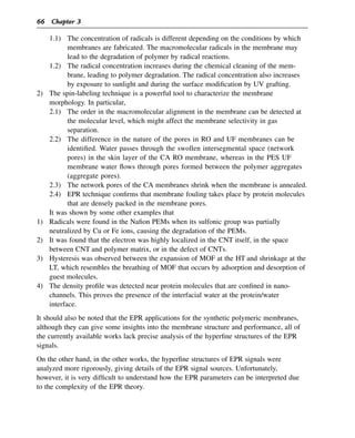
![As well, EPR technique has the following drawbacks compared to the other
characterization techniques.
1) It is impossible to obtain two-dimensional (2D) or three-dimensional (3D) images of
the membrane surface (and the cross-section) unlike scanning electron microscope,
transmission electron microscope, and atomic force microscope.
2) Currently, it is impossible to investigate the surface of the membrane separately from
the bulk, unlike FTIR-ATR, XPS, EDX, and contact angle measurement.
3) Hence, the data are affected by the bulk structures under the top surface layer that
governs the performance of the asymmetric membrane, similar to XRD, DSC, TGA,
and measurement of mechanical strength.
Thus, the complication involved in the theoretical interpretation of EPR, absence of 2D
and 3D images taken by the EPR technique and difficulty in the surface observation is
now hampering the wider usage of the EPR technique to investigate the synthetic
polymeric membrane despite its enormous potential to reveal the details of the membrane
structure.
References
[1] UC Davis ChemWiki, http://chemwiki.ucdavis.edu/Physical_Chemistry/Spectroscopy/Magnetic_
Resonance_Spectroscopies/Electron_Paramagnetic_Resonance/EPR%3A_Theory.
[2] What is EPR spectroscopy?: University of Texas at Austin. http://epr.cm.utexas.edu/WhatIsEPR.html.
[3] Khulbe KC, Hamad F, Feng C, Matsuura T, Gumi T, Palet C. ESR spectra of spin probe in PPO
membrane. Polymer 2003;44:695e701.
[4] Khulbe KC, Matsuura T. Characterization of synthetic membranes by Raman spectroscopy, electron spin
resonance, and atomic force microscopy; a review. Polymer 2000;41:1917e35.
[5] Khulbe KC, Chowdhury G, Matsuura T, Lamarche G. Characterization of PPO [poly(phenylene oxide) ]
powder and membranes from it by ESR technique. J Membr Sci 1997;123:9e15.
[6] Khulbe KC, Chowdhury G, Kruczek B, Vujosevic R, Matsuura T, Lamarche G. Characterization of the
PPO dense membrane prepared at different temperatures by ESR, atomic force microscope and gas
permeation. J Membr Sci 1997;126:115e22.
[7] Gumi T, Valiente M, Khulbe KC, Palet C, Matsuura T. Characterization of activated composite
membranes by solute transport, contact angle measurement, AFM and ESR. J Membr Sci
2003;212:123e34.
[8] Khulbe KC, Matsuura T, Lamarche G, Lamarche A-M, Choi C, Noh SH. Study of the structure of
asymmetric cellulose acetate membranes for reverse osmosis using electron spin resonance (ESR) method.
Polymer 2001;42:6479e84.
[9] Khulbe KC, Matsuura T, Singh S, Lamarche G, Noh SH. Study on fouling of ultrafiltration membrane by
electron spin resonance. J Membr Sci 2000;167:263e73.
[10] Khulbe KC, Matsuura T, Feng SCY. Study on cellulose acetate membranes for reverse osmosis and
polyethersulfone membranes for ultrafiltration by electron spin resonance technique. Desalination
2002;148:329e32.
[11] Khulbe KC, Feng C, Matsuura T, Lamarche G, Lamarche A-M. Study of the structure of asymmetric
polyamide membranes for reverse osmosis using the electron spin resonance (ESR) method. Desalination
2003;154:1e8.
Electron Paramagnetic Resonance (EPR) Spectroscopy 67](https://image.slidesharecdn.com/epr-spectroscopy-250607060036-53afcfd1/85/EPR-Spectroscopy-pdf-spectreral-techicque-90-320.jpg)
![[12] Oppenheim SF, Buettner GR, Dordick JS, Rodgers VGJ. Applying electron paramagnetic resonance
spectroscopy to the study of fouling in protein ultrafiltration. J Membr Sci 1994;96:289e97.
[13] Kwon Y-N, Leckie JO. Hypochlorite degradation of crosslinked polyamide membranes I. Changes in
chemical/morphological properties. J Membr Sci 2006;283:21e6.
[14] Oliveira FRP, Matos CT, Moura JJG, Portugal CAM, Crespo JG. Study of membrane ageing and grafting
mechanisms using electron paramagnetic resonance. Desalination Water Treat 2011;27:150e8.
[15] Kadirov MK, Bosnjakovic A, Schlick S. Membrane-derived fluorinated radicals detected by electron spin
resonance in UV-irradiated nafion and Dow ionomers: efffect of counterions and H2O2. J Phys Chem B
2005;109:7664e70.
[16] Yang HY, Han ZJ, Yu SF, Pey KL, Osrikov K, Karnik R. Carbon nanotube membranes with ultrahigh
specific adsorption capacity for water desalination and purification. Nat Commun 2013;4. http://dx.doi.org/
10.1038/ncomms3220. Article number: 2220.
[17] Hinds BJ, Chopra N, Rantell T, Andrews R, Gavalas V, Bachas LG. Aligned multiwalled carbon nanotube
membranes. Science 2004;303:62e5.
[18] Chipara M, Zaleski JM, Hui D, Du C, Pan N. Electron spin resonance on carbon nanotubes-polymer
composites. J Polym Sci Part B 2005;43:3406e12.
[19] Rao SS, Stesmans A, Noyen JV, Jacobs P, Sels B. Electron spin resonance investigation of ultra-small
double walled carbon nanotubes embedded in zeolite nanochannels. J Phys Condens Matter
2011;23:455801. 6 pp.
[20] Hartmann M, Kunz S, Himsl D, Tangermann O. Adsorptive separation of isobutene and isobutane on
Cu3(BTC)2. Langmuir 2008;24:8634e42.
[21] Mendt M, Jee B, Stock N, Ahnfeldt T, Hartmann M, Himsl D, Pöppl A. Structural phase transitions and
thermal hysteresis in the metalorganic framework compound MIL-53 as studied by electron spin
resonance spectroscopy. J Phys Chem C 2010;114:19443e51.
[22] Lai Y-C, Chen Y-F, Chiang Y-W. ESR study of interfacial hydration layers of polypeptides in water-filled
nanochannels and in vitrified bulk solvents. PLoS One 2013;8:e68264. p. 130.
[23] Taniguchi Y, Horigome S. The states of water in cellulose acetate membranes. J Appl Polym Sci
1975;19:2743e8.
68 Chapter 3](https://image.slidesharecdn.com/epr-spectroscopy-250607060036-53afcfd1/85/EPR-Spectroscopy-pdf-spectreral-techicque-91-320.jpg)
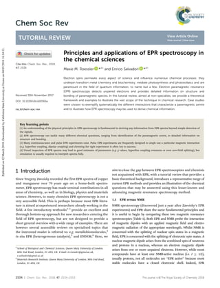
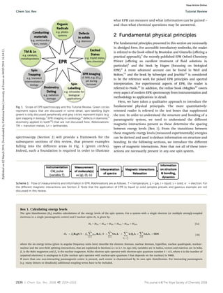
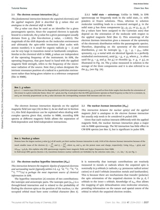
![2538 | Chem. Soc. Rev., 2018, 47, 2534--2553 This journal is ©The Royal Society of Chemistry 2018
Box 4. A more quantitative look at the hyperfine interaction
For an electron coupled to a single nuclear spin, the hyperfine Hamiltonian is given by:
HHF = SAI. (2)
The hyperfine matrix A consists of an isotropic and an anisotropic component:
A = aisoI + T, (3)
where I is the identity matrix and T is the dipolar part of the hyperfine matrix. aiso (typically in MHz), also known as Fermi’s contact interaction, is proportional
to the probability of finding the electron spin at the nucleus (|c(0)|2
):
aiso ¼
2m0
3
h
gebegnbn cð0Þ
2
¼
TrðAÞ
3
: (4)
It follows from eqn (4) that different isotopes of the same element will display isotropic hyperfine constants proportional to the corresponding gn, for instance
deuterium will have an isotropic hyperfine coupling B6.5 times smaller than that of hydrogen.
The dipolar part of the hyperfine matrix can be used to determine the distance r between an unpaired electron (T is proportional to 1/r3
). In the EPR literature,
A, aiso and T are usually given, where
A = [Ax, Ay, Az] = aiso + T. (5)
Ax,y,z are the principal components of the diagonalized hyperfine matrix and T = [T, T, 2T] in axial symmetry.
The anisotropic part (T) is a pure magnetic dipole–dipole
interaction that averages out in liquid solution and is thus only
detected in the solid state. T depends on the orientation and
the average distance between the unpaired electron and the
magnetically active nucleus. Like g in the solid state, T has
three components (Tx, Ty, Tz, along each Cartesian axis). In EPR,
Fig. 2 Energy level diagrams, transitions and field-swept EPR spectra to illustrate the (A) Zeeman interaction for a system with a single unpaired electron
(S = 1/2) and (B) hyperfine interaction with a I = 1/2 nucleus (e.g. 1
H). Hyperfine transitions are governed by the selection rules Dms = 1 (where
ms = +1/2 = a, ms = 1/2 = b, blue labels) and DmI = 0 (where mI = +1/2 = a, mI = 1/2 = b, green labels). In both Ai and Bi EPR transitions (blue doted
arrows) are only shown for the isotropic case, giving rise to lines in the corresponding blue CW EPR spectra shown in (Aii and Bii). In (Bi), the NMR
transitions (nuclear transition frequencies) in the a and b electron-spin manifolds are denoted with na and nb, respectively. The dotted line in Aii marks the
resonance position for a free electron at g = 2.0023. The equations describing the resonance conditions in each case are given above the corresponding
energy level diagram (nmw = applied microwave frequency). The insets in Aii and Bii depict the magnetic interactions at play. Note that giso (taken
arbitrarily as g = 1.93) is the average of 2g (1.80) and g8 (2.20); similarly, aiso (130 MHz) is the average of 2A (60 MHz) and A8 (270 MHz). CW spectra
were simulated using EasySpin (microwave frequency 9.6 GHz, linewidth 2 mT).
Chem Soc Rev Tutorial Review
Published
on
02
March
2018.
Downloaded
by
California
State
University
at
Fresno
on
04/05/2018
16:14:13.
View Article Online](https://image.slidesharecdn.com/epr-spectroscopy-250607060036-53afcfd1/85/EPR-Spectroscopy-pdf-spectreral-techicque-96-320.jpg)
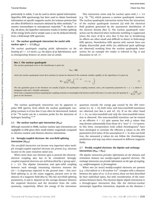
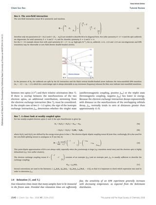
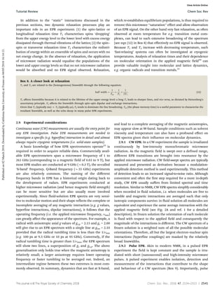
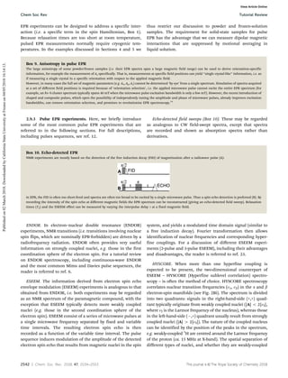
![This journal is ©The Royal Society of Chemistry 2018 Chem. Soc. Rev., 2018, 47, 2534--2553 | 2543
or strongly-coupled explains the popularity of HYSCORE. This
technique is however much more time-consuming than one-
dimensional ESEEM.
DEER. The double electron–electron resonance (DEER)
experiment is often the method of choice to measure the
distance between two weakly-coupled electron spins. It is a
two-frequency (pump and probe) experiment that measures the
electron dipole–dipole interaction between two spins, which
varies inversely with their cubed distance. The first microwave
frequency is used to select a fraction of the spins (probe) and to
produce the measured signal (echo). A second microwave
frequency (pump) is used to invert the orientation of the
coupled spin, causing a modulation of the signal (echo) inten-
sity at the frequency of the electron spin–spin coupling (known
as the dipolar frequency).
2.10 Spectral interpretation
Simulation is usually required for the interpretation of EPR spectra
but is increasingly accessible to non-specialists.
Few spectra can be fully and easily interpreted by measuring
peak positions and separations like in one-dimensional NMR (Box
11). Spectral interpretation is often the most time-consuming
aspect of any EPR study and usually requires simulation of the
EPR spectra. Historically, simulations were a major bottleneck,
with each research group having to develop their own pro-
grammes. Nowadays a number of excellent packages are available.
One of the best is EasySpin, a toolbox supported by MATLAB for
simulating and fitting CW and pulsed EPR spectra (http://easy
spin.org).24,25
The now widespread use of Easyspin, which is freely
available, enables consistent analysis and allows non-experts to
simulate most EPR spectra. EPR spectrometers manufacturers
have also developed simulation packages (e.g. XSophe by Bruker).
In addition, the fast open-source spin dynamics programme
Spinach covers magnetic resonance applications, including EPR
(http://spindynamics.org/Spinach.php).26
Finally, the on-line
educational tool EPR simulator (http://www.eprsimulator.org),†
enables the user to see the effect of different EPR parameters on
simulated spectra (e.g. Cu(II), nitroxides, radicals in solution) in
an interactive manner.
Box 11. Why is the interpretation of EPR spectra not straightforward?
EPR spectra often depend on the magnitude and relative orientation of all magnetic tensors (g, A, Q, D) with respect to each other and with respect to the
applied magnetic field. This leads to many parameters, but simulations often allow the determination of these tensors and their relative orientation.
In some cases (e.g. when many interactions are of similar magnitude), fitting of the experimental data based on a full quantum mechanical computation
(density functional theory) and molecular dynamics simulations is necessary for reliable spectral interpretation.
3 What g values can tell us and the
benefit of multiple frequencies (HEZ)
In this section we discuss how the interaction between a para-
magnet and the applied magnetic field leads to the appearance
of an EPR line at a characteristic g value that depends on the
molecular environment and the electronic ground state. Owing
to their dependence on spin–orbit coupling, g values are much
more difficult to predict than NMR chemical shift values and
tables correlating g with structural motifs are limited.27,28
Nonetheless, g values can be important parameters in EPR
characterisation. The relevance of g as an observable to char-
acterise the electronic state and molecular geometry, and the
detection of mechanistically-relevant bonding interactions is
illustrated below. The advantages of multi-frequency EPR to
disentangle composite spectra will also be apparent.
3.1 Detecting the presence of different species and deducing
electronic configurations
Motivated by the role that Ti(III) compounds play in homo-
geneous and heterogeneous catalysis (e.g. Ziegler–Natta poly-
merisation), Chiesa, Van Doorslaer and co-workers investigated
TiCl3(Py)3 and TiCl3 complexes.29
Continuous-wave EPR spectra
at multiple microwave frequencies (Fig. 3) revealed the presence
of two distinct rhombic Ti(III) ([Ar]3d1
, hence S = 1/2) species. The
g values of the peak positions remain unchanged with increasing
magnetic field, indicating that any magnetic interaction between
the centres is negligible (see, in contrast, Section 3.2). The two
Ti3+
species could in fact be ascribed to defects in the solid,
ligated by 14
N nuclei (as revealed by pulse EPR experiments,
not discussed here). In this case, the only magnetic interaction
that needs to be considered is the EZ interaction for the two
Ti(III) species since other interactions are not resolved (i.e. the
spin Hamiltonian is well described by HEZ, see eqn (1), Box 1).
Fig. 3 Two distinct Ti(III) species present in powder TiCl3(Py)3, as revealed
by multifrequency EPR. Simulated EPR spectra are in red. Adapted from
ref. 29 with permission from the PCCP Owner Societies.
† EPR Simulator is under construction and being developed by Dr Victor Chechik,
University of York (UK).
Tutorial Review Chem Soc Rev
Published
on
02
March
2018.
Downloaded
by
California
State
University
at
Fresno
on
04/05/2018
16:14:13.
View Article Online](https://image.slidesharecdn.com/epr-spectroscopy-250607060036-53afcfd1/85/EPR-Spectroscopy-pdf-spectreral-techicque-101-320.jpg)
![2544 | Chem. Soc. Rev., 2018, 47, 2534--2553 This journal is ©The Royal Society of Chemistry 2018
Note that the peaks appear sharper, on a g-value scale, at higher
microwave frequencies because they are further apart on a
magnetic field scale, while the linewidths do not increase
proportionally with the field. This is analogous to NMR experi-
ments carried out at different operating frequencies, where
however the effect is less apparent since NMR peaks are
generally much sharper (Section 1.1).
All six principal g values of the two Ti(III) species are below ge.
This illustrates that generally g o 2 for transition metal com-
plexes with configuration dn,no5
, conversely g 4 2 for dn,n45
and
g B ge for d5
complexes (e.g. high-spin Mn2+
). The relatively
large g anisotropy (Section 2.1) is a reflection of the effective
spin–orbit coupling constant that increases with increasing
nuclear charge (excited states are closer to the ground state).
g values can also yield information on the electronic ground
state and the geometry of metal complexes. A classic example is
Jahn–Teller distorted Cu2+
. The vast majority of Cu2+
complexes
exhibit a ‘lengthening’ of the z axis (tetragonal distortion),
resulting in the unpaired electron being in the 3dx2–y2 orbital
(gz 4 gx,y). Halcrow and co-workers30,31
have shown that simple
substitution by more bulky substituents in the ligand framework
can result in ‘shortening’ of the z axis (a much less common type
of tetragonal distortion), and thus in the unpaired electron being
in the 3dz2 orbital, i.e. gz o gx,y (see Fig. 4, left). This is clearly
apparent in the Q-band (B35 GHz) CW EPR spectra (Fig. 4,
right). Note that the hyperfine coupling of the electron spin to
the Cu nuclear spin (I = 3/2, 2I + 1 = 4) is, as is often the case,
only resolved along gz.
3.2 Inferring magnetic coupling between centres through
g values
EPR spectroscopy led to the discovery of iron–sulfur (Fe–S)
clusters, which are now recognised to be ubiquitous in nature
and assume a wide range of roles ranging from electron
transfer to participation in catalysis. It was long a puzzle how
two Fe ions (high-spin Fe3+
, S = 5/2, and Fe2+
, S = 2, both have
expected g values above ge) give rise to an average g value
below ge. Long before the first crystallographic structures
became available, Gibson et al.32
predicted an antiferromagnetic
exchange interaction between the Fe centres, forming a [2Fe–2S]
cluster, that explains the experimentally observed g values and the
total spin Stotal = SFe(III) SFe(II) = 1/2 ground state (Fig. 5).
3.3 Detecting mechanistically relevant bonding interactions
Radicals are involved in numerous redox reactions and biological
electron transfer, and deciphering their bonding interactions is of
mechanistic relevance. Stoll et al. showed that hydrogen bonding
to tryptophan radical cations is reflected in a change in the g
anisotropy.34
The very small shift of gx by just 0.00015 (Fig. 6), that
could be predicted by density functional theory, is only detectable
at extremely high magnetic fields/frequencies (700 GHz). Pulse
ENDOR (Section 2.9) at lower frequencies (X- and Q-band)
however could detect the H-bonded proton by comparison with
the deuterated sample. The very different magnetic properties
of 1
H (I = 1/2) and 2
H (I = 1) mean that deuteration is commonly
employed to detect and characterise exchangeable protons, and
the effects of isotopic substitution on EPR spectra are discussed
further in Section 4.4.
Fig. 4 Illustration of the g value serving as an observable to characterise the electronic ground state and molecular geometry. Note that in the axial case,
g8 is typically used to designate gx = gy and g = gz. Figure adapted from ref. 31 with permission from The Royal Society of Chemistry.
Fig. 5 The structure of a typical [2Fe–2S] cluster, as found in e.g. spinach
ferredoxin (left) and corresponding X-band EPR spectrum33
(right), illus-
trating that antiferromagnetic coupling between the Fe centres results
in a single unpaired electron with an average (isotropic) g value below ge.
Colour coding: Fe = orange, S = yellow, N = blue, O = red, protein
backbone = green.
Chem Soc Rev Tutorial Review
Published
on
02
March
2018.
Downloaded
by
California
State
University
at
Fresno
on
04/05/2018
16:14:13.
View Article Online](https://image.slidesharecdn.com/epr-spectroscopy-250607060036-53afcfd1/85/EPR-Spectroscopy-pdf-spectreral-techicque-102-320.jpg)
![This journal is ©The Royal Society of Chemistry 2018 Chem. Soc. Rev., 2018, 47, 2534--2553 | 2545
All discussion in this section was restricted to S = 1/2 systems.
Large deviations from ge can occur in systems with multiple
unpaired electrons (see Section 5).
4 Nuclei surrounding the unpaired
electron spin: Hyperfine and nuclear
quadrupole interactions (HHF HNQ)
In this section we will show that a wealth of information can be
extracted from the interaction between unpaired electrons
and surrounding nuclei, that not only encodes structural
but also functional and mechanistic information. In the
examples below, the reader will be introduced to some of the
most common experiments used to measure and gain more
detailed information from hyperfine interactions. More than a
single EPR method is often suitable (and necessary) to solve
a particular problem, and the examples below have been
chosen to illustrate different hyperfine EPR experiments (see
Section 2.9.3).
4.1 Fe(I) intermediate in catalysis (CW EPR)
Organometallic Fe(I) compounds are rare but were recently
shown to be important intermediates in Negishi cross-coupling
reactions through EPR experiments.35
Continuous-wave EPR
spectroscopy of a likely Fe(I) intermediate shows that the
unpaired electron is primarily located on the low-spin Fe centre
(S = 1/2), with a near-axial g tensor (Fig. 7) whose anisotropy was
reproduced in DFT calculations. Moreover, large hyperfine
couplings to four nearby phosphorus atoms (I = 1/2) are clearly
visible. From the 1 : 4 : 6 : 4 : 1 quintuplet pattern apparent in the
g1 region‡ and on the basis of the structure one may be led to
conclude that the strength of the hyperfine coupling to the Fe(I)
electron spin of the two (equal) equatorial P is very similar to
the two (equal) axial P. However, as revealed through
simulation of the entire EPR spectrum, the equatorial 31
P are
actually inequivalent and one is more weakly coupled (aiso =
37.9 MHz, T = [2.9, 5.7, 2.7] MHz, see Box 4) relative to the
remaining P ligands with similar coupling parameters (aiso =
71 MHz, T = [2.8, 1.4, 1.4] MHz). EPR experiments thus
demonstrated unambiguously that Fe(I) is present in such
cross-coupling reactions, and that the complex adopts a dis-
torted geometry in solution as shown by the inequivalent spin
density distribution onto the 31
P ligands.
4.2 Host–guest interactions (ENDOR)
Unless the hyperfine coupling to the electron spin is relatively
large (tens of MHz), it is often not observed in CW EPR in
the solid state. We now discuss an example of a much subtler
interaction. Turro and co-workers investigated the magnetic
communication between a fulleride radical anion host cage and
a H2 guest molecule encapsulated within it (Fig. 8). The H2
guest can be in the ortho (I = 1) or para (I = 0) nuclear
spin state.36
The CW EPR spectrum (Fig. 8A) is dominated by
three lines of approximately equal intensity, arising from the
unpaired electron delocalised over the surface of the fulleride
coupling to the nearby 14
N atom with I = 1 (additional low-
intensity lines arise from coupling to 13
C atoms of low natural
abundance). However, pulsed ENDOR spectroscopy revealed
the weak coupling between the unpaired electron and the
endo-H2 molecule through difference spectra (Fig. 8B). In this
‘‘weak-coupling case’’ (nI 4 A/2), the observed peaks are centred
around the Larmor frequency of the proton (nI E 14.8 MHz) at
the measurement field as shown in Fig. 8B (A = [0.35, 0.35,
1.00], i.e. aiso = 0.10 MHz and T = 0.45 MHz, see Box 4). On
the basis of the magnetic interaction between the fulleride and
the H2 molecule, demonstrating that cage and host molecule
‘communicate’, and the observed temperature dependence of
the ENDOR spectra (not discussed here) showing that the ortho–
para interconversion takes no longer than 1 hour, the authors
conclude that spin catalysis is highly efficient and may lead to a
new way of driving ortho-H2/para-H2 conversion.
Fig. 6 Illustration of how g values can be sensitive to relatively weak
bonding interactions. The gx of the tryptophan radical cation shifts
with hydrogen bonding, as revealed by very high-frequency EPR
(700 GHz). In deuterated samples the proton of HX (in red) is replaced
by D. Adapted with permission from ref. 34. Copyright 2011 American
Chemical Society.
Fig. 7 Fe(I) complex in Negishi cross-coupling reactions (left, schematic
structure) and corresponding X-band CW EPR spectrum and simulation
(right) demonstrating that the unpaired electron is mostly located on Fe.
Note that the indicated hyperfine couplings A are very approximate but
serve as a good starting point for simulations (a useful rule of thumb is that
1 mT B 28 MHz for g B 2). Adapted with permission from ref. 35.
Copyright 2012 American Chemical Society.
‡ Note the notation g1,2,3 (rather than gx,y,z) is used in this case because the g
values were not assigned to the Cartesian axes.
Tutorial Review Chem Soc Rev
Published
on
02
March
2018.
Downloaded
by
California
State
University
at
Fresno
on
04/05/2018
16:14:13.
View Article Online](https://image.slidesharecdn.com/epr-spectroscopy-250607060036-53afcfd1/85/EPR-Spectroscopy-pdf-spectreral-techicque-103-320.jpg)
![2546 | Chem. Soc. Rev., 2018, 47, 2534--2553 This journal is ©The Royal Society of Chemistry 2018
4.3 The interstitial atom in the nitrogenase MoFe cluster
(ESEEM)
The co-called MoFe cluster is one of the most complex clusters
found in nature and being paramount for ‘fixing’ N2 (breaking
the nitrogen triple bond to form ammonia), by a mechanism
that is not fully understood, continues to be an inspiration for
biochemists and chemists alike. The nature of the central
interstitial atom (formally coordinated by six bonds) was long
a debate that EPR spectroscopy has helped to resolve in con-
junction with high-resolution X-ray crystallography.37
Upon
labelling with 13
C (I = 1/2), ESEEM revealed a small hyperfine
coupling of 2.5 MHz (see inset in Fig. 9) centred around the
Larmor frequency peak of 13
C at 3.7 MHz, showing that the
central atom is, surprisingly, carbon.
4.4 Distinguishing between possible reaction intermediates
(HYSCORE)
HYSCORE spectroscopy can be used to elucidate catalytic
mechanisms and a powerful strategy is to combine HYSCORE with
isotopic labelling. This can allow detection of usually silent nuclei
(e.g. 12
C to 13
C, I = 1/2, substitution) or spectral simplification (e.g.
14
N, I = 1, to 15
N, I = 1/2, substitution). As seen is Section 2.8.3,
HYSCORE can distinguish between strongly and weakly coupled
nuclei, providing means to characterise intermediates structurally
and validate or rule out possible catalytic reaction pathways.
Fugate et al.38
used HYSCORE to distinguish between three
intermediates proposed to lead to the formation of biotin, an
essential vitamin. The structure of the intermediate deduced
from the spectroscopic data is composed of a reduced [2Fe–2S]
cluster with a total spin S = 1/2 ground state (see Section 3.2)
bonded to 9-mercaptodethiobiotin (MDTB) as shown in Fig. 10C.
Selective 13
C labelling of MDTB revealed signals (correlation
ridges), centred around the Larmor frequency of 13
C (3.8 MHz
at 355 mT), that were not visible in the natural-abundance
sample (Fig. 10A); the relatively large aiso (2.7 MHz, see Box 4)
shows that significant electron density is on the 13
C atom,
suggesting that it is directly bonded to the Fe–S cluster, as
corroborated by the relatively large axial anisotropy (T = 1.5 MHz,
Box 4). The simulated spectrum of the 13
C coupling (in the absence
of orientation selection, see Box 9) is shown in Fig. 10Aii (right) –
note that the experimental spectrum (Fig. 10Aii, left) shows only
part of the full ridge required to determine the hyperfine
parameters (and hence aiso and T) directly from the spectrum.
Indicative of the two inequivalent N in the side-chain
Arginine, the HYSCORE spectrum of the 15
N-Arg substituted
enzyme (Fig. 10Bii) shows the presence of two sets of peaks,
centred around A/2 in the left-hand quadrant (resulting from
the strongly-coupled blue N in Fig. 10C) and the Larmor
frequency of 15
N in right-hand quadrant (resulting from the
weakly-coupled green N in Fig. 10C), respectively. The corres-
ponding 14
N spectrum is considerably more complicated; up
to 18 cross-peaks may be observed owing to the quadrupole
moment arising from the I = 1 nucleus. Usually the most
prominent (often sole) peaks are those arising from the so-called
double-quantum (dq) transitions (DmI = 2 in each ms mani-
fold, Fig. 10D) and the hyperfine coupling A can be estimated
from these (Fig. 10Bi). Determining the nuclear quadrupole
parameters can be useful to deduce structural information such
as the degree of sp hybridisation and hence coordination of the
N nucleus in question.39
Although this is often a challenging
task, for the strongly-coupled 14
N in this example they are
readily obtained because the nuclear Zeeman and hyperfine
interactions are of similar magnitude and approximately cancel
each other out (i.e. combined they have no net effect on the
energy levels) in one of the ms manifolds (i.e. 2|nI| E |aiso|, here
Fig. 8 (A) CW EPR spectrum of the fulleride radical anion pictured in B with
endo-H2 (simulated spectrum in red). (B) Davies ENDOR EPR spectra of the
fulleride in the presence (black) and absence (red) of the endo-H2 molecule,
and the difference spectrum (blue), with simulation (red). Adapted with
permission from ref. 36. Copyright 2012 American Chemical Society.
Fig. 9 The MoFe cluster found in nitrogenases showing the usual central
C atom with nominally six bonds (left; colour coding: Fe = grey, S = yellow,
Mo = brown, central C = highlighted red, protein backbone = black, O = red,
N = dark blue) and 3-pulse ESEEM spectra in the frequency domain of the
wild-type (wt), 15
N- and 13
C-labelled protein. The inset show experiments
acquired at different t values (see Box 10); this is a requirement for 3-pulse
ESEEM experiments because these are affected by blind spots (a suppression
effect where individual peaks in the spectrum can disappear completely).
Adapted from ref. 37. Reprinted with permission from AAAS.
Chem Soc Rev Tutorial Review
Published
on
02
March
2018.
Downloaded
by
California
State
University
at
Fresno
on
04/05/2018
16:14:13.
View Article Online](https://image.slidesharecdn.com/epr-spectroscopy-250607060036-53afcfd1/85/EPR-Spectroscopy-pdf-spectreral-techicque-104-320.jpg)
![This journal is ©The Royal Society of Chemistry 2018 Chem. Soc. Rev., 2018, 47, 2534--2553 | 2547
the Larmor frequency of 14
N at field of the measurement, 347.5 mT,
is 1.1 MHz and aiso = 3.5 MHz), as illustrated in Fig. 10D. The
nuclear quadrupole transitions n0, n and n+ (n0 = 2KZ, n+ = K(3 + Z)
and n = K(3 + Z), where n0 + n = n+ and K = e2
qQ/4h (in MHz)
for I = 1, see also Box 5) are then directly observable (Fig. 10Bi)
and nuclear quadrupole parameters e2
qQ/h and Z can be
determined easily.40
This ‘‘cancellation’’ or ‘‘matching’’ condition
is surprisingly common for 14
N because it occurs even when 2|nI|
does not appear to match |aiso| very well. In fact, n0, n and n+ are
observed as long as |nI |aiso|/2|/K B 0.75–1 (in the example
given this ratio approaches the upper limit of 1). In many cases,
the condition can be deliberately achieved by changing the
microwave frequency.41
5 More than one unpaired electron
(HZFS, HDD and HEX)
For species with more than one unpaired electron (S 41/2) the
mutual interaction between the unpaired electrons must be
considered. High-spin centres are common for transition metals
and organic chromophores excited to their triplet (or higher
order) state with laser irradiation, and these will be the focus of
our discussion here. Pairs of weakly interacting spins (2 S = 1/2)
engineered onto diamagnetic molecules represent a special case
of multiple unpaired electrons and are becoming increasingly
popular in structural biology for distance determination.
5.1 Metal centres
Owing to their partially occupied d orbitals, transition metals
often possess unpaired electrons and are thus amenable to EPR
studies. In the EPR literature, low-spin refers to S = 1/2 systems
whereas high-spin pertains any S 4 1/2 system; the terminology
thus differs from that of coordination chemistry (e.g. a ‘‘low-spin’’
d4
octahedral complex is termed a high-spin S = 1 system in EPR).
When there is a considerable exchange interaction between two or
more spins (e.g. two metal centres sharing a m-oxo bridge or two
radicals covalently linked together) it is often convenient to define
a total spin Stotal. If spins are ferromagnetically coupled, Stotal is
the sum of the individual spins. For anti-ferromagnetically
coupled spins, Stotal is the difference of the individual spins (see
Sections 3.2 and 5.1.2 for examples).
Integer spins (S = 1, 2. . .) are often difficult to observe in
standard (parallel-mode) EPR because the zero-field splitting
(ZFS, Section 2.6, Box 6) usually exceeds the energy of the
microwave photons and their study typically requires high
microwave frequencies beyond the conventional X- to W-bands.
The ZFS varies greatly amongst different metal ions and coordi-
nation geometries as it depends on the spin–orbit coupling
(see Section 3.1 for the effect of spin–orbit coupling on g), for
instance it is very small for symmetric Mn(II) complexes and very
large for octahedral Co(II) complexes. A comprehensive review
on (high-field) EPR of mononuclear transition metal complexes
can be found in ref. 42.
Fig. 10 Spectroscopic evidence for the [2Fe–2S]-MDTB intermediate in the biosynthetic pathway of biotin. (Ai and Bi) HYSCORE spectra of the native protein
bound to MDTB. (Aii) Left: HYSCORE spectrum with 13
C-labelled MDTB and (Aii) right: simulated spectrum for the 13
C coupling in the absence of orientation
selection. (Bii) HYSCORE spectrum with 15
N-labelled arginine; note that in this case, the hyperfine parameters from the strongly-coupled 15
N can be estimated
quite accurately from the spectrum, despite orientation selection. (C) Spectroscopically deduced structure of the [2Fe–2S]-MDTB intermediate. (D) Energy-
level diagram for a 14
N nucleus in the ‘cancellation’ condition. Adapted with permission from ref. 38. Copyright 2012 American Chemical Society.
Tutorial Review Chem Soc Rev
Published
on
02
March
2018.
Downloaded
by
California
State
University
at
Fresno
on
04/05/2018
16:14:13.
View Article Online](https://image.slidesharecdn.com/epr-spectroscopy-250607060036-53afcfd1/85/EPR-Spectroscopy-pdf-spectreral-techicque-105-320.jpg)
![2548 | Chem. Soc. Rev., 2018, 47, 2534--2553 This journal is ©The Royal Society of Chemistry 2018
5.1.1 Interaction between multiple spins (exchange coupling).
With the goal to employ molecular nanomagnets as possible
qubits (a qubit is a quantum bit of information) Winpenny,
McInnes and co-workers used supramolecular chemistry to link
two {Cr7Ni} heterometallic rings (Stotal = 1/2, due to antiferromag-
netic coupling between 7 Cr(III) ions (S = 3/2), and 1 Ni(II) (S = 1),
Fig. 11B) to a Co(II) complex (S = 3/2). In this three-spin system, the
central Co atom is exchange coupled to the neighbouring {Cr7Ni}
heterometallic rings (Fig. 11A). EPR was used to determine the
weak interactions between molecular components in the supra-
molecular structure that are undetectable using magnetometry.
The ZFS of the central cobalt is too large to allow detection of inter-
manifold EPR transitions (see Box 6, even at 94 GHz). The Co2+
complex can be treated as an ‘effective’ S = 1/2 system with
‘characteristic’ g values that differ greatly from ge: gz = 6.5 (occur-
ring at B1000 mT in Fig. 11C), gy = 4.3 (B1600 mT) and gx E 2
(B3500 mT). The two heterometallic rings give rise to EPR signals
at gx,y = 1.78 and gz = 1.74, that partially overlap with the gx signal of
the Co(II) centre (Fig. 11C). The four additional splittings (a doublet
of doublets) of gz and gy are a manifestation of the anisotropic
exchange coupling (see Box 7) in the three-spin system and their
values can be estimated from the spectrum.
5.1.2 Structural analysis of unusual Fe–S clusters (ZFS
parameters, D E). Hydrogenases are enzymes that catalyse
the interconversion of protons and hydrogen and are a
benchmark for efficient H2 production with earth-abundant
metals. HydG, an enzyme required for the assembly of [FeFe]-
hydrogenases, harbours two [4Fe–4S] clusters. One of these is
instrumental for the synthesis of the [FeFe] active site and can
reversibly coordinate a fifth Fe atom yielding an unprecedented
[5Fe–5S] cluster. The addition of a Fe2+
(S = 2) centre to a [4Fe–4S]+
cluster (with Stotal = 1/2 in this case) generates a new spin
system with total spin either S = 5/2 (ferromagnetic coupling) or
S = 3/2 (antiferromagnetic coupling). The [5Fe–5S] and [4Fe–4S]
clusters are readily distinguishable in the CW EPR spectrum:
The high-spin [5Fe–5S] cluster (a mixture of S = 3/2 and 5/2)
appears at low magnetic field (Fig. 12A) whereas the low-spin
[4Fe–4S] cluster (S = 1/2) appears around g = 2 (Fig. 12B).44
With
the aid of the corresponding rhombogram for a S = 5/2 spin
system (Section 2.6), the four effective g values observed for
Fig. 11 Determining interactions in a nanomagnet using EPR. (A) Schematic structure of the supramolecular three spin complex. The exchange coupling
constants are indicated for each spin pair. (B) Structure of the polymetallic ring. In (A and B) Cr and Ni are represented as green and silver spheres,
respectively. (C) Experimental W-band (94 GHz) spectra of the three spin system at 5 K (black line) and corresponding simulation (red line). The exchange
coupling pattern along gz and gy is indicated. Adapted from ref. 43.
Fig. 12 EPR spectroscopic characterisation of the [5Fe–5S] cluster in the
assembly of [FeFe]-hydrogenases. (A) Low-field region of the X-band CW
EPR spectrum (10 K) showing evidence of a high-spin [5Fe–5S] cluster with
spin S = 5/2 (simulation in red) and 3/2 (simulation in blue). (B) High-field
region showing the [4Fe–4S] S = 1/2 cluster. (C) Exchange coupling
scheme for the formation of the S = 5/2 [5Fe–5S] cluster. (D) Partial
rhombogram for S = 5/2, showing effective g values for the ms = 3/2
intradoublet transitions when E/D = 0.225 (1/2 and 5/2 intradoublet
transitions not shown). Adapted from ref. 4 and 44.
Chem Soc Rev Tutorial Review
Published
on
02
March
2018.
Downloaded
by
California
State
University
at
Fresno
on
04/05/2018
16:14:13.
View Article Online](https://image.slidesharecdn.com/epr-spectroscopy-250607060036-53afcfd1/85/EPR-Spectroscopy-pdf-spectreral-techicque-106-320.jpg)
![This journal is ©The Royal Society of Chemistry 2018 Chem. Soc. Rev., 2018, 47, 2534--2553 | 2549
the [5Fe–5S] cluster are readily assigned: g = 9.5 arises from the
ms = 1/2 manifold (i.e. one of the ms = 1/2 - ms = +1/2
transitions)§ and g = 4.7, 4.1, 3.8 arise from the transitions
within the ms = 3/2 manifold (i.e. ms = 3/2 - ms = +3/2, in
different orientations), from which the rhombicity can be
determined as E/D = 0.225 (Fig. 12D). EPR spectroscopy thus
provided evidence for the usual [5Fe–4S] cluster whose high-
spin nature enabled its characterisation without interference
from the low-spin [4Fe–4S] cluster.
5.2 Light induced phenomena
Time-resolved EPR (TREPR) enables the investigation of light-
induced events such as photo-redox reactions, formation of
photoexcited triplet states and radical pairs,45
and homolytic
dissociation of chemical bonds. A laser flash generates the
paramagnetic species (e.g. triplet or radical) and pulsed EPR
experiments (i.e. detecting the electron spin echo, see Box 10) in
the excited state can be performed as well as CW EPR. In this
section, we provide an introduction to triplet-state EPR spectra
and discuss examples. For further literature in the field, the
reader is referred to ref. 46.
5.2.1 Introduction to triplet-state EPR spectra. Let us
consider a chromophore in its ground singlet state with an
allowed optical absorption. Upon absorption of a photon, the
chromophore is excited to its first excited singlet state. This can
either decay back to the ground state (fluorescence or non-
radiative decay) or cross to a triplet state via the intersystem
crossing (ISC) mechanism. Triplet states are characterised by
two unpaired electrons with parallel spins (S = 1) with three
corresponding triplet sublevels X, Y, Z. The triplet sublevels are
labelled as X, Y, Z in zero field and as 0, 1 in high field, since
the ms quantum number is meaningful only at high field
(Fig. 13A and C). Since ISC is an anisotropic process, the
transitions from the singlet excited state to the three triplet
sublevels (and the decay rates from the three triplet sublevels to
the ground singlet state) generally have different probabilities
as determined by the molecular symmetry. Consequently, the
populations of the triplet sublevels do not follow the Boltzmann
distribution and are said to be spin polarised. Moreover, even
in the absence of an applied field the energies of the triplet
sublevels are usually non-degenerate and the relative splittings
depend on the ZFS parameters (Section 2.6), as sketched in
Fig. 13B. The corresponding transitions can be probed directly
in zero-field and the most common way for organic triplet
states is optically detected magnetic resonance.47
When an external field is applied as customary in EPR, the
electron Zeeman interaction also needs to be considered.
Fig. 13C shows the energy level diagram for the simple case
of the applied magnetic field parallel to the Z sublevel, in the
assumption that the electron Zeeman interaction is much
larger than all other interactions. The energy of this sublevel
does not depend on the strength of the applied field, whereas
the energy of the other sublevels mix and split proportionally to
the applied field strength. Similar considerations apply to the
Fig. 13 Illustration of the origin of triple-state EPR spectra. (A) Formation of a triplet via intersystem crossing from the first excited singlet. The
populations of the three sublevels are represented with green circles and do not follow the Boltzmann distribution. (B) EPR transitions in zero field. The
ordering of the energy levels depends on the sign of the ZFS parameters; in the case illustrated D, E 4 0. (C) In presence of an applied field two allowed
EPR transitions can be observed for each molecular orientation (here B0 is parallel to the Z axis of the ZFS tensor). (D) EPR spectrum corresponding to (C).
(E) Simulated powder-average EPR spectrum for the isotropic case. A = enhanced absorption; E = emission.
§ Note that the other two g values are not observed because these are {1.
Tutorial Review Chem Soc Rev
Published
on
02
March
2018.
Downloaded
by
California
State
University
at
Fresno
on
04/05/2018
16:14:13.
View Article Online](https://image.slidesharecdn.com/epr-spectroscopy-250607060036-53afcfd1/85/EPR-Spectroscopy-pdf-spectreral-techicque-107-320.jpg)