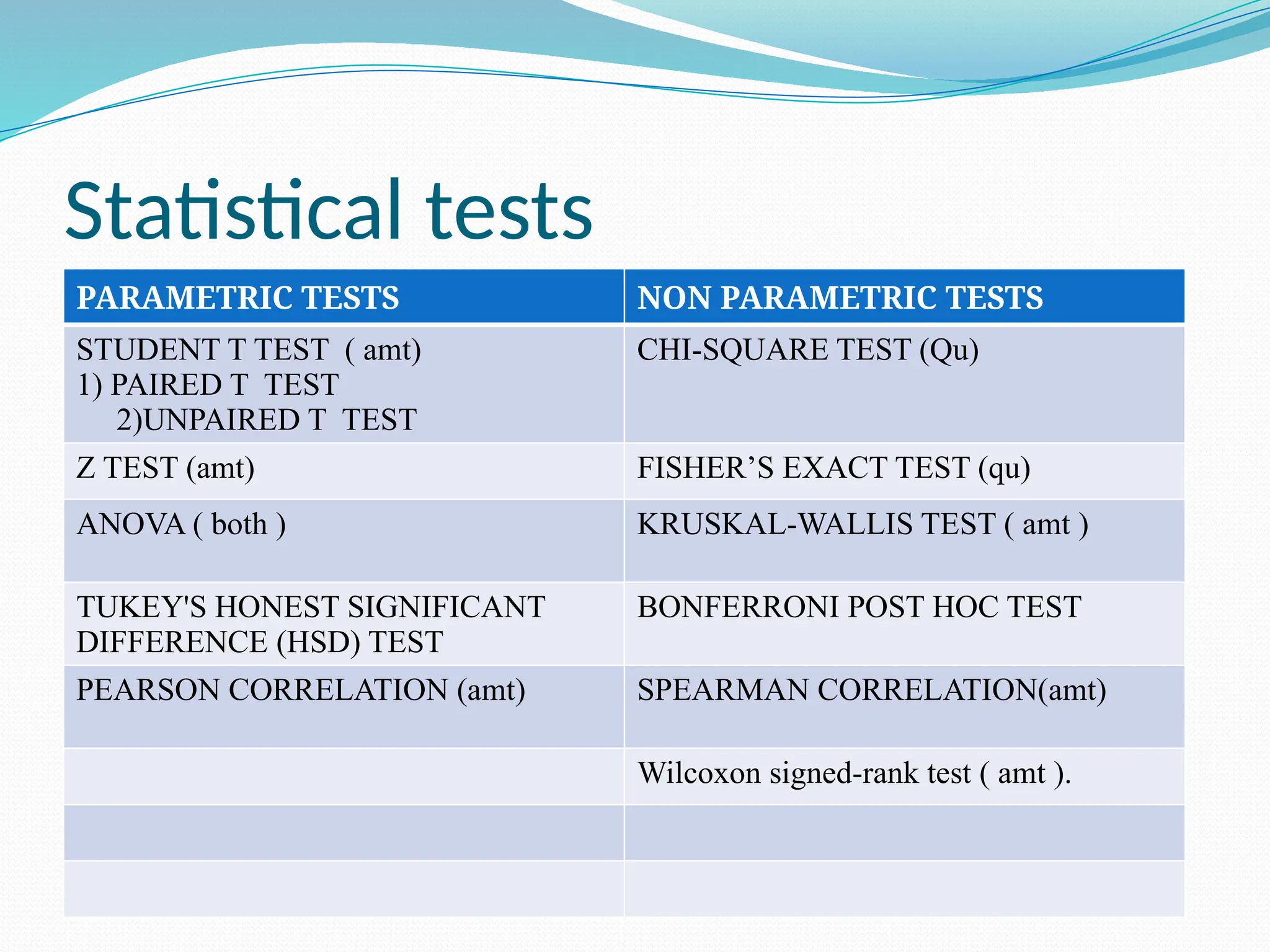
The document discusses various statistical tests used to analyze data, focusing on tests of significance, p-values, and confidence intervals. It explains different types of errors, including Type I and Type II errors, and various statistical methods like the paired t-test, unpaired t-test, chi-square test, ANOVA, and correlation coefficients. Additionally, the document details applications such as the Wilcoxon signed-rank test and the use of ROC curves for evaluating binary classifiers.

1. Dr Ashish
PG first Yr.
Dept. of Biochemistry
Kcgmc karnal
STATISTICAL TESTS

2. TEST OF SIGNIFICANCE
 A test of significance is a statistical method used to determine whether the observed
data in an experiment or study are strong enough to reject a null hypothesis. The
null hypothesis typically represents a default assumption, such as no effect or no
difference between groups.
 The test assesses the probability that the observed results would occur if the null
hypothesis were true. This probability is represented by the p-value.

3. Confidence Interval (CI)
• A confidence interval gives a range of values within which we expect the true
population parameter (like the mean) to fall, based on our sample data.
• confidence interval 95% :This tells us we are 95% confident that the interval we
calculate from our sample data includes the true population parameter.( like the
mean)

5. p- Value
 It is a standard against which we compare our result
 It is a result of computation
 Computed p-value compared with p-value criterion to test statistical significance
 Smaller p-value is always better
 p≤0.05 means reject null hypothesis and reached statistical significance
 p>0.05 means do not reject null hypothesis and has not reached statistical
significance

6. Types of error
 Type I error/ alpha error- rejecting the null hypothesis when it is true (error of
commission)
 Actually no difference, but test saying there is difference
 Worse than beta
 Asserts that drug works, when it does not
 Type II/ beta error- failing to reject null hypothesis when it is false (error of
omission)
 Actually there is difference, but test saying there is no difference
 Asserts that drug does not work, when it really does

7. Statistical tests
PARAMETRIC TESTS NON PARAMETRIC TESTS
STUDENT T TEST ( amt)
1) PAIRED T TEST
2)UNPAIRED T TEST
CHI-SQUARE TEST (Qu)
Z TEST (amt) FISHER’S EXACT TEST (qu)
ANOVA ( both ) KRUSKAL-WALLIS TEST ( amt )
TUKEY'S HONEST SIGNIFICANT
DIFFERENCE (HSD) TEST
BONFERRONI POST HOC TEST
PEARSON CORRELATION (amt) SPEARMAN CORRELATION(amt)
Wilcoxon signed-rank test ( amt ).

8. Paired t-Test and
Unpaired t-Test
Photo by Pexels

9. Paired T-test
Purpose: The paired t-test is used when you have two measurements taken on the
same group of subjects under different conditions or at different times. It assesses
whether the mean difference between the paired observations is significantly different
from zero.
When to Use:
•When you have two related samples (e.g., before and after measurements on the
same individuals).
•When you want to evaluate the effect of a treatment or intervention within the same
group.

10. Example: Suppose a researcher wants to evaluate the effect of a new diet on weight loss. They
measure the weight of 10 participants before starting the diet and then again after 6 weeks on the
diet. The weights are paired because each participant is measured twice, once before and once after
the diet.
•Before Diet (Weight in kg): 80, 85, 90, 95, 100, 105, 110, 115, 120, 125
•After Diet (Weight in kg): 78, 82, 88, 93, 98, 102, 108, 112, 118, 123
In a paired t-test, you would calculate the differences between the paired weights (Before - After) for
each participant and then test if the mean of these differences is significantly different from zero.

11. •Paired t-test: Compares means from the same group at different times or conditions.
Use it for repeated measures or matched samples.
•Unpaired t-test: Compares means between two independent groups. Use it when the
groups are unrelated.
Both tests assume that the data are normally distributed.
Difference between Paired t-test and unpaired t-test

12. 1. Paired t-test Calculation
Example Data
Before Diet (Weight in kg): 80, 85, 90, 95, 100, 105, 110, 115, 120, 125
After Diet (Weight in kg): 78, 82, 88, 93, 98, 102, 108, 112, 118, 123

13. Steps:
1.Calculate the differences between the paired observations.
Differences (Before - After):
80 - 78 = 2
85 - 82 = 3
90 - 88 = 2
95 - 93 = 2
100 - 98 = 2
105 - 102 = 3
110 - 108 = 2
115 - 112 = 3
120 - 118 = 2
125 - 123 = 2
Differences: 2, 3, 2, 2, 2, 3, 2, 3, 2, 2

15. * Degree of freedom in statistics reflect the number of independent values in a data set
that can vary without breaking any constraints imposed by the statistical model or
estimation method.

16. Z test
A Z-test is a statistical test used to determine whether there is a significant difference
between the means of two groups, or to compare a sample mean to a known population
mean when the population variance is known and the sample size is large (typically
n>30). The Z-test relies on the assumption that the data follows a normal distribution.
Testing Enzyme Activity
Let's say we are studying an enzyme that catalyzes a specific biochemical reaction.
We know from previous studies that the average activity level of this enzyme in a
healthy population is 50 units per milliliter (U/mL) with a known standard deviation of
5 U/mL.

17. Hypothesis:
We suspect that a new drug has an effect on the enzyme's activity. After administering
the drug to a sample of 40 patients, we measure the enzyme activity and find an
average activity of 52 U/mL.
Objective:
To determine whether the observed increase in enzyme activity is statistically
significant or just due to random chance, you perform a Z-test.
Steps in the Z-Test:
1) Formulate Hypotheses:
Null Hypothesis (H0): The mean enzyme activity after drug administration is 50
U/mL (no effect). μ=50
Alternative Hypothesis (H1​
): The mean enzyme activity after drug administration
is different from 50 U/mL (effect present). μ≠50

19. Determine the Critical Value: For a significance level (alpha) of 0.05 in a two-tailed
test, the critical Z-value is ±1.96.
Make a Decision:
If Z > 1.96, reject the null hypothesis.
Since 2.53 > 1.96, you reject the null hypothesis.
Conclusion:
The Z-test shows that the enzyme activity after drug administration is significantly
different from the known average of 50 U/mL. This suggests that the drug likely has
an effect on enzyme activity.
This approach is useful in biochemistry when comparing enzyme activities,
concentrations of biomolecules, or other measurable parameters to known standards

20. ANOVA
 ANOVA (Analysis of Variance) is a statistical method used to compare the means of
three or more groups to determine if there is a statistically significant difference
between them.
 ANOVA is particularly useful when you have multiple groups and want to test
whether their means are all equal or if at least one group differs significantly from
the others.
 ANOVA can be used for both qualitative and quantitative data.

21. How ANOVA Works:
1. Null Hypothesis (H ):
₀ Assumes that all group means are equal.
2. Alternative Hypothesis (H ): Assumes that at least one group mean is different.
₁
3. F-Statistic: ANOVA calculates an F-statistic, which is a ratio of the variance
between group means to the variance within the groups. A larger F-statistic indicates a
greater difference between group means relative to the variance within groups.
4. p-value: The F-statistic is used to determine the p-value, which helps decide
whether to reject the null hypothesis. A low p-value (typically < 0.05) suggests that
there is a statistically significant difference between the group means.

22. Correlation
To find out linear relation between two variables eg height and weight, temp
and pulse etc.
In order to find out whether there is significant association or not between two
variables ( we may call them x and y) we calculate Co-efficient of correlation,
represented by “rxy”.

23.  Suppose, we have two variables x and y and we have individuals who
have each one reading of x and one reading of y. the correlation
coefficient is given by the formula

24. Correlation analysis
Correlation coefficient (r), which ranges from -1.0 to +1.0
1. +ve value= two variable go together in same direction
E. g.= age and atherosclerosis
2. -ve value=increase in value of one variable associated with decrease in value of
another variable E. g.=age and quick reflexes
3. 0 value= no linear correlation between 2 variables
E. g.=height and school grade of children

25. 1. Pearson Correlation
Type: Parametric
Description: Measures the linear relationship between two continuous variables. It
assumes that the data is normally distributed and that the relationship between the
variables is linear.
Use: The Pearson correlation coefficient (r) ranges from -1 to 1, where:
r = 1 indicates a perfect positive linear relationship.
r= −1 indicates a perfect negative linear relationship.
r=0 indicates no linear relationship.
Test: Pearson's correlation test is used to determine whether there is a significant linear
relationship between two continuous variables

26. Spearman's Rank Correlation
Type: Non-parametric
Description: Measures the strength and direction of the relationship between two
ranked variables. It does not assume a linear relationship or normally distributed data.
Use: The Spearman correlation coefficient ρ or rs ranges from -1 to 1, similar to
Pearson, but it is based on the ranks of the data rather than the actual values.
Test: Spearman's rank correlation test is used to assess the association between two
variables when the data is ordinal, not normally distributed.

27. Regression
 To know in an individual case the value of one variable, knowing the value
of other.
 We calculate regression coefficient of one measurement to the another.
 We denote independent variable as x
and dependent variable as y.

28. The value of b is called regression coefficient of y upon x

29. Similarly, we can obtain regression of x upon y. Where b1
is regression coefficient of x upon y. The function of regression is to provide means of estimating the value of one variable
from the another.

30. Chi-square Test
 To determine if there is a significant association between two categorical variables.
 To find a relationship between a treatment type and the presence or absence of a certain
disease.
 Example: Determine if there is an association between receiving a COVID-19 vaccine
and health outcomes (healthy vs. non-healthy) among a sample of individuals.
Data Collection
Vaccination Status Healthy Non-Healthy Total
Vaccinated 150 30 180
Unvaccinated 80 40 120
Total 230 70 300

31.  Procedure:
1. Formulate Hypothesis Null Hypothesis (H0 ) and alternate hypothesis (H1)

32. Null Hypothesis (H0):
There is no association between vaccination status and health outcome.
Alternative Hypothesis (H1):
There is an association between vaccination status and health outcome.
Step 1: Formulate Hypotheses

33. Step 2: Calculate Expected Frequencies
Vaccination Status Healthy Non-Healthy Total
Vaccinated 150 30 180
Unvaccinated 80 40 120
Total 230 70 300

34. Step 3: Compute the Chi-Square Statistic
Healthy Non-Healthy
Vaccination Status Oij Eij Oij Eij Total
Vaccinated 150 138 30 42 180
Unvaccinated 80 92 40 28 120
Total 230 70 300

35. Step 4: Determine Degrees of Freedom

36.  Check the published probability table,
 On referring to Table, with 1 degree of freedom, the value
of for a probability of 0.05 is 3.84
 Since the calculated chi-square statistic (11.18) is greater than
the critical value (3.841), we reject the null hypothesis.
 We accept the alternate Hypothesis.
Step 5: Compare the chi-square statistic with the critical value
Χ2
Χ2
Chi-square Table

37. Interpretation
 Alternate hypothesis: there is a statistically significant
association between vaccination status and health outcome.
 This suggests that receiving the COVID-19 vaccine is
associated with a higher likelihood of being healthy compared
to those who are unvaccinated.

38. The Kruskal-Wallis test
The Kruskal-Wallis test is a non-parametric statistical test used to determine if there
are statistically significant differences between the medians of three or more
independent groups.
It is the non-parametric alternative to the One-Way ANOVA and is particularly useful
when the assumptions of ANOVA, such as normality and homogeneity of variance, are
not met.
This can be used to compare three or more independent groups or samples.

39. Hypotheses:
- Null Hypothesis (H ): The medians of the different groups are equal.
₀
- Alternative Hypothesis (H ): At least one group has a median different from the
₁
others.
How the Kruskal-Wallis Test Works:
1. Ranking the Data:
- Combine all the data from the groups into a single dataset.
- Rank the data from the lowest to the highest, assigning ranks to the data points. If there
are ties, assign the average rank to the tied values.


40. 2. Calculating the Test Statistic:
- The test statistic for the Kruskal-Wallis test is denoted as (H).
- H is calculated using the sum of ranks for each group, the number of observations in each
group, and the total number of observations across all groups.
3. Determining Significance:
- The H statistic is compared to a chi-square distribution with ( k-1 ) degrees of freedom, where
k is the number of groups.
- A p-value is obtained, and if this p-value is less than a predefined significance level (e.g., 0.05),
the null hypothesis is rejected, indicating that there is a significant difference in the medians of the
groups.

41. Steps in the Kruskal-Wallis Test:
1. Combine and Rank Data:
- Example: Suppose you are comparing the effectiveness of three different diets on weight loss in three groups
of participants:
- Group A (Diet A): 5, 7, 6
- Group B (Diet B): 8, 9, 7
- Group C (Diet C): 4, 3, 5
- Combine the data: [5, 7, 6, 8, 9, 7, 4, 3, 5]
- Rank the data: [3, 4, 5, 5, 5, 6, 7, 7, 8, 9]
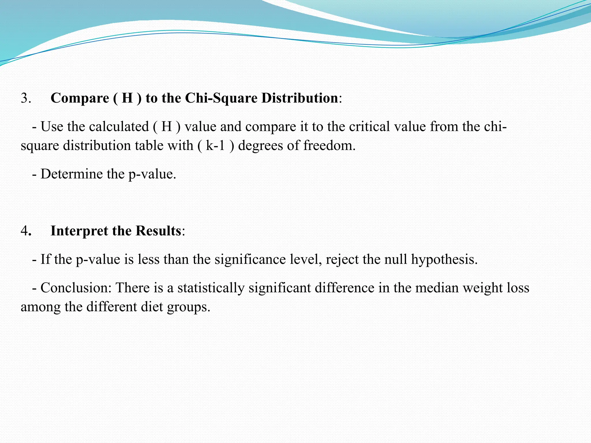
2. Calculate the Test Statistic (H):
- Calculate the sum of ranks for each group.
- Compute the ( H ) statistic using the Kruskal-Wallis formula.

42. 3. Compare ( H ) to the Chi-Square Distribution:
- Use the calculated ( H ) value and compare it to the critical value from the chi-
square distribution table with ( k-1 ) degrees of freedom.
- Determine the p-value.
4. Interpret the Results:
- If the p-value is less than the significance level, reject the null hypothesis.
- Conclusion: There is a statistically significant difference in the median weight loss
among the different diet groups.

43. Wilcoxon signed-rank test
 The Wilcoxon signed-rank test is a non-parametric statistical test used to compare
two related samples, matched samples, or repeated measurements on a single
sample to assess whether their population mean ranks differ.
 It's a popular alternative to the paired t-test when the data cannot be assumed to be
normally distributed.

44.  How It Works:
1. Calculate Differences: For each pair of observations, calculate the difference
between the two related samples.
2. Rank the Differences: Rank the absolute values of these differences, ignoring any
differences that are zero.
3. Assign Signs to the Ranks: Assign the original signs (+ or -) of the differences to
the ranks.

45. 4) Sum the Ranks: Sum the ranks separately for the positive and negative differences.
5) Test Statistic: The test statistic W is the smaller of the absolute values of these two
sums (positive and negative ranks).
6) Compare to Critical Value or Compute p-value: This test statistic is then
compared to a critical value from the Wilcoxon distribution table, or a p-value is
computed to determine the significance of the test.

46. Significance
Assessing Changes: The Wilcoxon signed-rank test is used to assess whether there is a
statistically significant change in a population’s median between two conditions. For
example, it can determine if a treatment has a significant effect on a group of patients
when comparing pre-treatment and post-treatment scores.
When to Use: This test is particularly useful when the assumptions of the paired t-test
are not met, such as when the data is ordinal, not normally distributed, or when dealing
with outliers that could affect the results of a parametric test.
Interpreting Results: A significant result (p-value < 0.05, for example) suggests that
there is a difference in the median ranks of the two samples, implying that the
treatment or intervention had an effect.

47. Receiver Operating Characteristic (ROC)/ ROC
curve
 is a graphical plot which illustrates the performance of a
binary classifier system.
 It is created by plotting the fraction of true positives/ sensitivity(Y-
axis) vs. the fraction of false positives/ (1-specificity)(X-axis), at
various threshold settings.
 In general, if both values are known, the ROC curve can be drawn.

48. Types - ROC curves representing excellent, good, and worthless tests plotted on
the same graph.
The accuracy of the test depends on how well the test separates the group being
tested into those with and without the disease in question. Accuracy is measured
by the area under the ROC curve
An area of 1 represents a perfect test; an area of .5 represents a worthless
test. A rough guide for classifying the accuracy of a diagnostic test is the
traditional academic point system:
 .90-1 = excellent (A)
 .80-.90 = good (B)
 .70-.80 = fair (C)
 .60-.70 = poor (D)
 .50-.60 = fail (F)

49. Sensitivity and Specificity

52. THANKS
Thank you