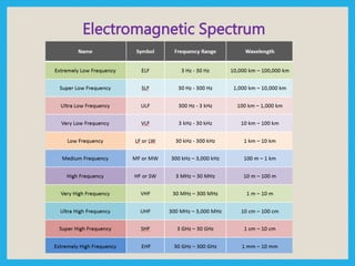
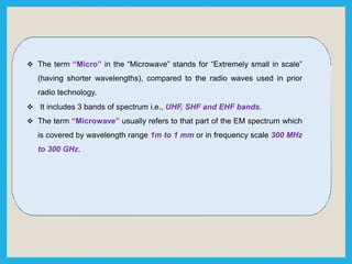
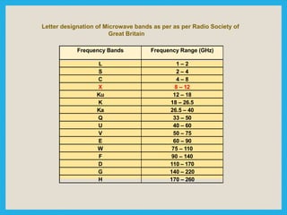
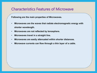
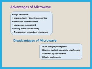
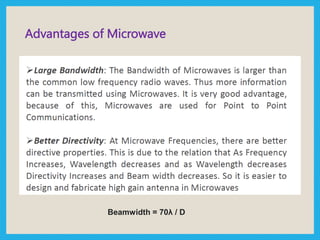
Electromagnetic Spectrum & Transmission line Theory

Microwaves &
Transmission Line
Theory
Presented By:
Prof. Shailaja Udtewar
Department of EXTC
Xavier Institute of Engineering, Mumbai

Electromagnetic Spectrum
The term “Spectrum” was first introduced in the 17th century to explain the
range of colours observed when white light is passed through a prism.
It was soon applied to other waves like sound waves, electromagnetic
waves etc.
Now it is applied to any signal that can be decomposed into frequency
components.
“EM Spectrum” refers the range of all possible frequencies of EM
radiations and it extends from low frequencies, used for Radio
Communication to higher end at Gama radiation. Alternatively it covers
wavelengths from thousands of km down to the fraction of the size of an
atom.

 The term “Micro” in the “Microwave” stands for “Extremely small in scale”
(having shorter wavelengths), compared to the radio waves used in prior
radio technology.
 It includes 3 bands of spectrum i.e., UHF, SHF and EHF bands.
 The term “Microwave” usually refers to that part of the EM spectrum which
is covered by wavelength range 1m to 1 mm or in frequency scale 300 MHz
to 300 GHz.

Letter designation of Microwave bands as per as per Radio Society of
Great Britain
Frequency Bands Frequency Range (GHz)
L 1 – 2
S 2 – 4
C 4 – 8
X 8 – 12
Ku 12 – 18
K 18 – 26.5
Ka 26.5 – 40
Q 33 – 50
U 40 – 60
V 50 – 75
E 60 – 90
W 75 – 110
F 90 – 140
D 110 – 170
G 140 – 220
H 170 – 260

Characteristics Features of Microwave
Following are the main properties of Microwaves.
• Microwaves are the waves that radiate electromagnetic energy with
shorter wavelength.
• Microwaves are not reflected by Ionosphere.
• Microwaves travel in a straight line.
• Microwaves are easily attenuated within shorter distances.
• Microwave currents can flow through a thin layer of a cable.

Advantages of Microwave
High bandwidth
Improved gain / directive properties
Reduction in antenna size
Low power requirement
Fading effect and reliability
Transparency property of microwave
Disadvantages of Microwave
Line of sight propagation
Subject to electromagnetic interference
Affected by bad weather
Costly equipments

Beamwidth = 70λ / D

• Antenna gain also has a direct correlation to both antenna
directivity and beamwidth.
• Higher gain antennas achieve extra power by focusing on a
reduced area; thus, the greater the gain, the smaller the area
covered (measured in degrees of beamwidth).
• Antenna gain and beamwidth always are inversely proportional.

 Fading effect and reliability:
At microwaves fading is less on the signal transmission but at LF
due to the transmission medium fading is more
 Power requirements:
These are partly low for both transmission and reception at
microwave frequencies
 Transparency property :
From 300MHz to 10 GHz signals are capable of freely propagating
through the ionized layers surrounding the earth as well as
through the atmosphere like duplex .comm... exchange of
information

Applications of Microwave
Radio detection and ranging
Terrestrial microwave link
Transmission of many television channels over one link
Satellite communication
Radio astronomy
Linear particle accelerator
Studies on basic properties of materials
Microwave oven
Industry
Medical Science

Limitations of Microwave
• Up to around a frequency of 1 GHz, most circuits are designed and
constructed using lumped parameter circuit components.
• Above 1 GHz the propagation time of the signal becomes comparable with
the time period of the signal.
• The lumped parameter circuit component length also becomes comparable
to the wavelength.
• This results in a rapid amplitude and phase variation of the signal with the
distance.
• The phase difference caused by the interconnection of different
components is also not negligible above 1 GHz.
• As a result at high frequencies KCL, KVL and normal voltage-current
concepts are not applicable. Instead field theory is required.

• Above 1 GHz the lumped circuit elements are replaced by the
distributed circuit element.
• The distributed circuit elements are small transmission line sections and the
are defined over an infinitesimal length.
• In this model the connecting wires between different elements are not
perfect conductor.
• At high frequencies the distributed circuit model is more accurate than the
lumped element circuit model and also more complex in nature.
• The existence of non-uniform current in the branches and non-uniform
voltages at the nodes further complicates the analysis of the circuit.
• The use of infinitesimals in distributed circuit model requires the application
of calculus rather than linear algebra.
Distributed circuit theory

Lumped Elements
• If the size of an element is smaller than the wavelength of the
applied signals, then it is a lumped element.
• In lumped elements, the effect of wave propagation can be
neglected.
• The physical dimensions of lumped elements make it so that signals
do not vary over the interconnects interfacing them.
• There are only minimal phase differences between the input and
output signals in lumped elements.
• Generally, the size of lumped elements is less than 1/20 times the
operating guided wavelength.
• Examples of lumped elements include:
• Resistors
• Capacitors
• Inductors

Distributed Elements
• The physical dimension of distributed elements is comparable with
the operating wavelength.
• They are distributed over lengths in an RF or microwave circuit.
• When conventional lumped elements are difficult to implement at
microwave frequencies, distributed elements are used instead.
• They perform the same functions as lumped elements, but the
signals vary along the lines and between the elements.
• These signals undergo considerable phase change across various
points within the distributed elements.
• Examples of distributed elements include:
• Stubs
• Coupled lines
• Cascaded lines

TRANSMISSION LINE
Introduction:
◦ In an electronic system, the delivery of power requires the
connection of two wires between the source and the load.
◦ At low frequencies, power is considered to be delivered to the load
through the wire.
◦ In the microwave frequency region, power is considered to be in
electric and magnetic fields that are guided from Place to place by
some physical structure.
◦ Any physical structure that will guide an electromagnetic wave place
to place is called a Transmission Line.

CHOICE OF TRANSMISSION LINES
◦ In practice, the choice of structure is dictated by:
(a) the desired operating frequency band,
(b) the amount of power to be transferred, and
(c) the amount of transmission losses that can be tolerated.

TYPES OF TRANSMISSION LINES
There are basically four types of transmission lines −
1. Two wire line
2. Coaxial cable
3. Waveguide
 Rectangular
 Circular
4. Planar Transmission Lines
 Strip line
 Microstrip line
 Slot line
 Fin line
 Coplanar Waveguide
 Coplanar slot line

◦ Coaxial cables are widely used to connect RF components.
◦ Their operation is practical for frequencies below 3 GHz. Above
that the losses are too excessive.
◦ For example, the attenuation might be 3 dB per 100 m at 100
MHz, but 10 dB/100 m at 1 GHz, and 50 dB/100 m at 10 GHz.
◦ Their power rating is typically of the order of 1KW at 100 MHz,
but only 200 W at 2 GHz, being limited primarily because of the
heating of the coaxial conductors and of the dielectric between
the conductors (dielectric voltage breakdown is usually a
secondary factor.)

◦ Another issue is the single-mode operation of the line.
◦ At higher frequencies, in order to prevent higher modes from being
launched, the diameters of the coaxial conductors must be reduced,
diminishing the amount of power that can be transmitted.
◦ Two-wire lines are not used at microwave frequencies because they
are not shielded and can radiate.
◦ One typical use is for connecting indoor antennas to TV sets.
Microstrip lines are used widely in microwave integrated circuits.

Waveguides are used to transfer electromagnetic power efficiently from
one point in space to another.
y
x
z
Coaxial line
Two-wire line
Microstrip line
Rectangular waveguide Dielectric waveguide
WAVEGUIDES

TRANSMISSION LINE PARAMETERS
◦ A transmission line is a connector which transmits energy from
one point to another.
◦ While transmitting or while receiving, the energy transfer has to
be done effectively, without the wastage of power.
◦ To achieve this, there are certain important parameters which has
to be considered.
◦ Primary Constants
◦ Secondary Constants

PRIMARY CONSTANTS
◦ The four electric circuit parameters R, L, G and C associated with the
transmission lines are referred to as primary constants of the
transmission lines.
1. Resistance: The series resistance is contributed by the conductors
themselves and depends upon their diameter and length. The
resistance is uniformly distributed along the length of the transmission
line. It is denoted by R and measured in ohms per unit length of
transmission line.
2. Inductance: The series inductance is contributed by the magnetic field
of each conductor carrying a current. The inductance is also uniformly
distributed along the length of the transmission line. It is denoted by L
and measured in henries per unit length of the transmission line.

PRIMARY CONSTANTS
3. Capacitance: The shunt capacitance is contributed by the two
conductors, placed parallel or twisted and separated by a dielectric.
The capacitance is also distributed along the length of the
transmission line. It is denoted by C and measured in farads per unit
length of the transmission line.
4. Conductance: The dielectric in between the conductor is not perfect.
Hence, a small conduction current or leakage current flows in
between the wires. This results in the shunt conductance. It exists
between the conductor and distributed along the length of the
transmission line. It is denoted by G and measured in mho per unit
length of the transmission line.

PRIMARY CONSTANTS
◦ The important parameters of a transmission line are resistance,
inductance, capacitance and conductance.
◦ Resistance and inductance together are called as transmission
line impedance.
◦ Capacitance and conductance together are called as admittance.

SECONDARY CONSTANTS
◦ Secondary constants of a transmission line are referred to as
characteristic impedance (Zo) and propagation constant (γ) which can
be derived from primary constants.
◦ Though these parameters are generally applicable to all types of
transmission lines, they also help us in understanding phenomena like
reflections and wave propagation along a power transmission line

CHARACTERISTIC IMPEDANCE
◦ The characteristic impedance of a uniform transmission line is the
ratio of the amplitudes of voltage and current of a single wave
propagating along the line i.e a wave traveling in one direction in the
absence of reflections in the other direction.
◦ It can also be defined as the input impedance of a transmission line
when its length is infinite.
◦ It is denoted by Z0
◦ The SI unit of characteristic impedance is the ohm.

• A transmission line drawn as two black wires.
• At a distance x into the line, there is current phasor I(x) traveling through
each wire, and there is a voltage difference phasor V(x) between the wires.
• If Z0 is the characteristic impedance of the line, then
• Z0 =V(x)/I(x) for a wave moving rightward, or
• Z0 = - V(x)/I(x) or a wave moving leftward

• Lossless and lossy transmission lines have different characteristics that are
dependent upon the impedance in the transmission line.
• If the transmission line is lossy, the characteristic impedance is a complex
number.
• If the transmission line is lossless, the characteristic impedance is a real
number.

PROPAGATION CONSTANT
◦ The propagation constant of a sinusoidal electromagnetic wave is a
measure of the change undergone by the amplitude and phase of the
wave as it propagates in a given direction.
◦ The quantity being measured can be the voltage, the current in a circuit,
or a field vector such as electric field strength or flux density.
◦ It is denoted by γ

REFLECTIONS
◦ Reflections are nothing but reflected incident waves when a transmission
line has discontinuous impedance (mismatched impedance).
◦ In other words, if a line is not uniform throughout the whole length, the
incident wave (i.e., signal sent from source to load) will reflect to its origin
(source) instead of travelling all the way to the far end (load). This is what
they call reflections.
◦ These reflections are opposite to the incident waves, and they have adverse
effects on a transmission line such as, generating standing waves on the
line, attenuation in travelling waves (incident waves), and as a result, power
loss in transmission lines.
◦ There will be no reflections and no standing waves on a transmission line if
it is terminated in its characteristic impedance.

STANDING WAVES
Green signal = incident wave
Blue signal = reflected wave
Red signal = standing wave (they are generated due to interference
between incident and reflected wave along a line)
When a transmission medium through which a wave is traveling changes, it
experiences partial transmittance and partial reflectance. This behavior of
waves is best explained by reflection and transmission coefficient.

REFLECTION COEFFICIENT
◦ It is a parameter that describes how much of an incident wave is being
reflected due to impedance discontinuity in a transmission line.
◦ It is denoted by capital gamma (Γ) and can be calculated by the ratio of the
amplitude of reflected wave to the amplitude of incident wave.
◦ Reflection coefficient can be mathematically represented by,
◦ Reflection coefficient value is 0 for Matched load, -1 for Short circuit load
and +1 for Open circuit load

VOLTAGE STANDING WAVE RATIO
◦ When the resistive load termination is not equal to the characteristic
impedance, part of the power is reflected back and the remainder is
absorbed by the load.
◦ The amount of voltage reflected back is called voltage reflection
coefficient.
◦ The standing wave is formed when the incident wave gets reflected.
◦ The standing wave which is formed, contains some voltage.
◦ The magnitude of standing waves can be measured in terms of standing
wave ratios.

VOLTAGE STANDING WAVE RATIO (VSWR)
◦ The larger the impedance mismatch, the higher will be the amplitude of
the standing wave.
◦ Therefore, if the impedance is matched perfectly VSWR is unity, which
means the transmission is perfect.

STANDING WAVES
◦ A standing wave is formed by the addition of incident and reflected waves and has nodal
points that remain stationary with time.
◦ Voltage Standing Wave Ratio:
VSWR = Vmax/Vmin
◦ Voltage standing wave ratio expressed in dB is called the Standing Wave Ratio:
SWR (dB) = 20log10VSWR
◦ The maximum impedance of the line is given by:
Zmax = Vmax/Imin
◦ The minimum impedance of the line is given by:
Zmin = Vmin/Imax
◦ Relationship between VSWR and Reflection Coefficient:
VSWR = (1 + | Г | ) / (1 - | Г |)
Г = (VSWR – 1)/(VSWR + 1)

STANDING WAVES
◦ A reflection coefficient (
) with a magnitude of zero is a perfect match, a
value of one is perfect reflection.
◦ Unlike VSWR, the reflection coefficient can distinguish between short
and open circuits.
◦ A short circuit has a value of -1 (1 at an angle of 180 degrees), while an
open circuit is one at an angle of 0 degrees.

TRANSMISSION LINE TERMINATIONS
◦ Line terminated in its characteristic impedance: If the end of the
transmission line is terminated in a resistor equal in value to the
characteristic impedance of the line as calculated by the formula
Z=(L/C)0.5 , then the voltage and current are compatible and no
reflections occur.
◦ Line terminated in a short: When the end of the transmission line is
terminated in a short (RL = 0), the voltage at the short must be equal to
the product of the current and the resistance.
◦ Line terminated in an open: When the line is terminated in an open, the
resistance between the open ends of the line must be infinite. Thus the
current at the open end is zero.

◦ Fig below shows a lossless transmission line terminated in an arbitrary
load impedance ZL .

◦ This problem will illustrate wave reflection on transmission lines, a
fundamental property of distributed systems.
◦ Assume that an incident wave of the form is generated from
a source at z < 0.
◦ The ratio of voltage to current for such a traveling wave is Z0, the
characteristic impedance of the line.
◦ However, when the line is terminated in an arbitrary load ZL = Z0, the
ratio of voltage to current at the load must be ZL
◦ Thus, a reflected wave must be excited with the appropriate amplitude
to satisfy this condition.

◦ The total voltage on the line can then be written as a sum of incident
and reflected waves:

(SHORT CIRCUIT)

(OPEN CIRCUIT)

IMPEDANCE MATCHING
◦ To achieve maximum power transfer to the load, impedance matching has to be
done.
◦ To achieve this impedance matching, the following conditions are to be met.

STUB MATCHING
◦ If the load impedance mismatches the source impedance, a method called
"Stub Matching" is sometimes used to achieve matching.
◦ The process of connecting the sections of open or short circuit lines called
stubs in the shunt with the main line at some point or points, can be termed
as Stub Matching.
◦ At higher microwave frequencies, basically two stub matching techniques
are employed.
◦ Single Stub Matching
◦ Double stub Matching

SINGLE STUB MATCHING
◦ In Single stub matching, a stub of certain fixed length is placed at some
distance from the load.
◦ It is used only for a fixed frequency, because for any change in frequency,
the location of the stub has to be changed, which is not done.
◦ This method is not suitable for coaxial lines.

DOUBLE STUB MATCHING
◦ In double stud matching, two stubs of variable length are fixed at certain
positions.
◦ As the load changes, only the lengths of the stubs are adjusted to achieve
matching.
◦ This is widely used in laboratory practice as a single frequency matching
device.
◦ The following figures show how the stub matchings look.

LOW AND HIGH FREQUENCY
◦ At low frequencies, the circuit elements are lumped since voltage and
current waves affect the entire circuit at the same time.
◦ At microwave frequencies, such treatment of circuit elements is not
possible since voltage and current waves do not affect the entire
circuit at the same time.
◦ The circuit must be broken down into unit sections within which the
circuit elements are considered to be lumped.
◦ This is because the dimensions of the circuit are comparable to the
wavelength of the waves according to the formula:
l = c/f
where,
c = velocity of light
f = frequency of voltage/current

Electromagnetic Spectrum & Transmission line Theory

More Related Content

What's hot

Similar to Electromagnetic Spectrum & Transmission line Theory

Recently uploaded

Electromagnetic Spectrum & Transmission line Theory