DEPT & SEM:
SUBJECT NAME:
COURSE CODE :
UNIT :
PREPARED BY :
COURSE: MWE UNIT: 1 Pg. 1
ECE & I SEM
MICROWAVE ENGINEERING
MWOC
I
Mr. M Mahesh
2.
COURSE: MWE UNIT:1 Pg. 2
OUTLINE
• What is MICROWAVE?
• History of MICROWAVES
• Frequency Bands, EM Spectrum
• Microwave Advantages, Applications
• Waveguide Types, Field components of Rectangular waveguide
• TM Mode Analysis
• TE Mode Analysis
• Waveguide Parameters
• Cavity Resonator, Power Transmission and losses
• Microstriplines
3.
COURSE: MWE UNIT:1 Pg. 3
WHAT IS MICROWAVE
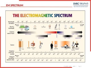
Microwaves are the electromagnetic waves whose frequencies rang from 1GHz to
1000GHz. Micro waves are also called as tinyness (small) waves due to their wave length
that is in terms of 1 meter to 1millimeter.
ranging from as long as one meter to as short as one millimeter, or equivalently
broad definition in terms of frequencies between 300 MHz and 300 GHz according to
electro magnetic spectrum.
A definite relationship exists between the frequency (f) and the corresponding wavelength
(λ) of electromagnetic waves .T
he product of these two i.e. (f) and (λ) gives the velocity of propagation of electro-
magnetic waves and it is equal to the velocity of light .
This is expressed as c = f * λ
c= velocity of light. (approx. 3* 108 m/sec ).
INTRODUCTION TO MICROWAVE:
4.
COURSE: MWE UNIT:1 Pg. 4
4
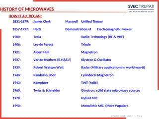
1831-1879: James Clerk Maxwell Unified Theory
1857-1937: Hertz Demonstration of Electromagnetic waves
1900: Tesla Radio Technology (HF & VHF)
1906: Lee de Forest Triode
1921: Albert Hull Magnetron
1937: Varian brothers (R.H&S.F) Klystron & Oscillator
1939: Robert Watson Watt Radar (Military applications in world war-II)
1940: Randoll & Boot Cylindrical Magnetron
1943: Kompfner TWT (helix)
1960: Twiss & Schneider Gyrotron, solid state microwave sources
1970: Hybrid MIC
1990: Monolithic MIC (More Popular)
HISTORY OF MICROWAVES
HOW IT ALL BEGAN:
5.
COURSE: MWE UNIT:1 Pg. 5
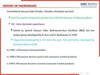
HISTORY OF MICROWAVES
Conventional Vacuum tube (Triodes, Tetrodes, Pentodes) was best
Can’t be used for frequencies greater than 100 MHz because of following effects
IEC –Inter electrode capacitance
Solved by Special Vacuum Tube: Barkhausen-Kurz Oscillator (BKO) but low
output power developed by K. Kurz and H. Barkhausen in 1920
Magnetron developed by A. W. Hull in the year 1921 and further developed by
Randoll & Boots in1939.
In 1960’ s Microwave Communication
In 1980’s Microwave devices used in the consumer market products
n 1990’s Microwave became common consumer market products
6.
COURSE: MWE UNIT:1 Pg. 6
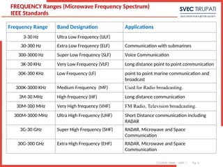
FREQUENCY Ranges (Microwave Frequency Spectrum)
IEEE Standards
Frequency Range Band Designation Applications
3-30 Hz Ultra Low Frequency (ULF)
30-300 Hz Extra Low Frequency (ELF) Communication with submarines
300-3000 Hz Super Low Frequency (SLF) Voice Communication
3K-30 KHz Very Low Frequency (VLF) Long distance point to point communication
30K-300 KHz Low Frequency (LF) point to point marine communication and
broadcast
300K-3000 KHz Medium Frequency (MF) Used for Radio broadcasting.
3M-30 MHz High frequency (HF) Long distance communication
30M-300 MHz Very High frequency (VHF) FM Radio, Television broadcasting.
300M-3000 MHz Ultra High Frequency (UHF) Short Distance communication including
RADAR
3G-30 GHz Super High Frequency (SHF) RADAR, Microwave and Space
Communication
30G-300 GHz Extra High Frequency (EHF) RADAR, Microwave and Space
Communication
7.
COURSE: MWE UNIT:1 Pg. 7
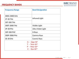
FREQUENCY BANDS
Frequency Range Band Designation
300G-3000 GHz
Infrared Light
3T-30 THz
30T-300 THz
300T-3000 THz Visible Light
3P-30 PHz Ultra Violet Light
30P-300 PHZ X-Rays
300P-3000 PHz Gamma Rays
3E-30 EHz Cosmic Rays
G - Giga-109
T - Tera-1012
P - Peta-1015
E - Exa-1018
8.
COURSE: MWE UNIT:1 Pg. 8
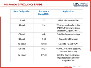
MICROWAVE FREQUENCY BANDS
Band Designation Frequency
Range(GHz)
Applications
L band 1-2 GSM, Marine satellite
S band 2-4 Weather and surface ship
RADAR, Microwave oven,
Bluetooth, ZigBee, Wi-Fi.
C band 4-8 Satellite Communication
X band 8-12 Educational Purpose
Ku band 12-18 Satellite TV and VSAT
K band 18-27 RADAR, Armature Satellite,
Infrared Astronmy
Ka band 27-40 Satellite Communication,
High resolution and low
range RADAR
COURSE: MWE UNIT:1 Pg. 14
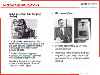
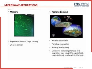
ADVANTAGES OF MICROWAVES
Large Bandwidth:
The Bandwidth of Microwaves is larger than the common low frequency radio waves.
Thus more information can be transmitted using Microwaves. It is very good advantage,
because of this, Microwaves are used for Point to Point Communications.
Improved Directivity:
As frequency increases , directivity increases and bandwidth decreases. Hence the
bandwidth of radiation θ is directly proportional to λ/D. At low frequency bands, the
size (diameter) of the antenna becomes very large if it is requires to get sharper beams
of radiation. B=1400
/(D/λ)
Transparency Window: Microwave frequency band ranging from 300 MHZ – 10 GHZ
are capable of freely propagating through the ionized layers surrounding the earth as
well as through the atmosphere.
1
15.
COURSE: MWE UNIT:1 Pg. 15
Power Consumption: The power required to transmit a high frequency signal is
lesser than the power required in transmission of low frequency signals. As
Microwaves have high frequency thus requires very less power.
Effect Of Fading Reliability: The effect of fading is minimized by using Line Of Sight
propagation technique at Microwave Frequencies. While at low frequency signals, the
layers around the earth causes fading of the signal
WAVEGUIDE:
A hollow metallic tube of the uniform cross section for transmitting electromagnetic
waves by successive reflections from the inner walls of the tube is called as a
Waveguide.
Microwaves propagate through microwave circuits, components and devices, which
act as a part of Microwave transmission lines, broadly called as Waveguides.
16.
COURSE: MWE UNIT:1 Pg. 16
WAVEGUIDE
A waveguide is generally preferred in microwave communications. A waveguide is a
special form of a transmission line, which is a hollow metal tube. Unlike the
transmission line, the waveguide has no center conductor.
ADVANTAGES OF WAVEGUIDES:
Waveguides are easy to manufacture.
They can handle very large power (in kilowatts)
Power loss is very negligible in waveguides
They offer very low loss ( low value of alpha-attenuation)
The microwave energy when travels through the waveguide, experiences lower
losses than a coaxial cable
17.
COURSE: MWE UNIT:1 Pg. 17
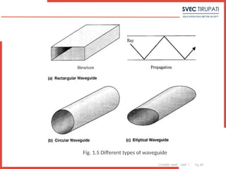
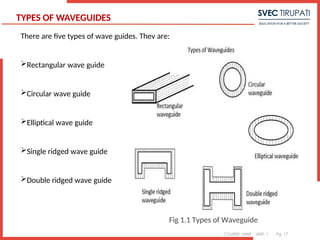
TYPES OF WAVEGUIDES
There are five types of wave guides. They are:
Rectangular wave guide
Circular wave guide
Elliptical wave guide
Single ridged wave guide
Double ridged wave guide
1
Fig 1.1 Types of Waveguide
18.
COURSE: MWE UNIT:1 Pg. 18
TRANSMISSION LINES VS WAVEGUIDES
1
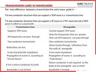
The main difference between a transmission line and a wave guide is −
A two conductor structure that can support a TEM wave is a transmission line.
A one conductor structure that can support a TE wave or a TM wave but not a TEM
wave is called as a waveguide.
Transmission Lines Waveguides
Supports TEM wave Cannot support TEM wave
All frequencies can pass through
Only the frequencies that are greater
than cut-off frequency can pass through
Two conductor transmission One conductor transmission
Reflections are less
Wave travels through reflections from
the walls of waveguide
It has characteristic impedance It has wave impedance
Propagation of waves is according to
"Circuit theory"
Propagation of waves is according to
"Field theory"
It has a return conductor to earth
Return conductor is not required as the
body of the waveguide acts as earth
Bandwidth is not limited Bandwidth is limited
19.
COURSE: MWE UNIT:1 Pg. 19
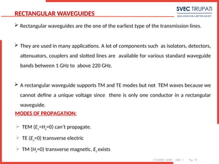
RECTANGULAR WAVEGUIDES
Rectangular waveguides are the one of the earliest type of the transmission lines.
They are used in many applications. A lot of components such as isolators, detectors,
attenuators, couplers and slotted lines are available for various standard waveguide
bands between 1 GHz to above 220 GHz.
A rectangular waveguide supports TM and TE modes but not TEM waves because we
cannot define a unique voltage since there is only one conductor in a rectangular
waveguide.
1
MODES OF PROPAGATION:
TEM (Ez=Hz=0) can’t propagate.
TE (Ez=0) transverse electric
TM (Hz=0) transverse magnetic, Ez exists
20.
COURSE: MWE UNIT:1 Pg. 20
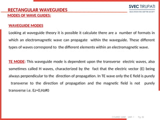
MODES OF WAVE GUIDES:
WAVEGUIDE MODES
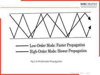
Looking at waveguide theory it is possible it calculate there are a number of formats in
which an electromagnetic wave can propagate within the waveguide. These different
types of waves correspond to the different elements within an electromagnetic wave.
TE MODE: This waveguide mode is dependent upon the transverse electric waves, also
sometimes called H waves, characterized by the fact that the electric vector (E) being
always perpendicular to the direction of propagation. In TE wave only the E field is purely
transverse to the direction of propagation and the magnetic field is not purely
transverse i.e. Ez=0,Hz#0
2
RECTANGULAR WAVEGUIDES
21.
COURSE: MWE UNIT:1 Pg. 21
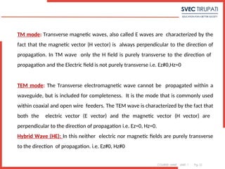
TM mode: Transverse magnetic waves, also called E waves are characterized by the
fact that the magnetic vector (H vector) is always perpendicular to the direction of
propagation. In TM wave only the H field is purely transverse to the direction of
propagation and the Electric field is not purely transverse i.e. Ez#0,Hz=0
TEM mode: The Transverse electromagnetic wave cannot be propagated within a
waveguide, but is included for completeness. It is the mode that is commonly used
within coaxial and open wire feeders. The TEM wave is characterized by the fact that
both the electric vector (E vector) and the magnetic vector (H vector) are
perpendicular to the direction of propagation i.e. Ez=0, Hz=0.
Hybrid Wave (HE): In this neither electric nor magnetic fields are purely transverse
to the direction of propagation. i.e. Ez#0, Hz#0
22.
COURSE: MWE UNIT:1 Pg. 22
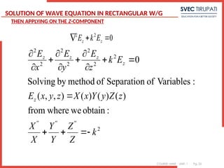
THEN APPLYING ON THE Z-COMPONENT
0
2
2
z
z E
k
E
2
2
2
2
2
2
2
2
:
obtain
we
where
from
)
(
)
(
)
(
)
,
,
(
:
Variables
of
Separation
of
method
by
Solving
0
k
Z
Z
Y
Y
X
X
z
Z
y
Y
x
X
z
y
x
E
E
k
z
E
y
E
x
E
''
''
''
z
z
z
z
z
SOLUTION OF WAVE EQUATION IN RECTANGULAR W/G
23.
COURSE: MWE UNIT:1 Pg. 23
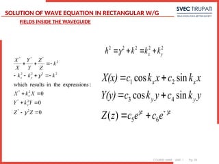
FIELDS INSIDE THE WAVEGUIDE
0
0
0
:
s
expression
in the
results
which
2
2
2
2
2
2
2
2
Z
Z
Y
k
Y
X
k
X
k
k
k
k
Z
Z
Y
Y
X
X
''
y
''
x
''
y
x
''
''
''
z
z
y
y
x
x
e
c
e
c
z
Z
y
k
c
y
k
c
Y(y)
x
k
c
x
k
c
X(x)
6
5
4
3
2
1
)
(
sin
cos
sin
cos
2
2
2
2
2
y
x k
k
k
h
SOLUTION OF WAVE EQUATION IN RECTANGULAR W/G
24.
COURSE: MWE UNIT:1 Pg. 24
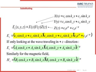
Substituting
z
z
y
y
x
x
e
c
e
c
z
Z
y
k
c
y
k
c
Y(y)
x
k
c
x
k
c
X(x)
6
5
4
3
2
1
)
(
sin
cos
sin
cos
)
(
)
(
)
(
)
,
,
( z
Z
y
Y
x
X
z
y
x
Ez
z
y
y
x
x
z
z
y
y
x
x
z
z
z
y
y
x
x
z
e
y
k
B
y
k
B
x
k
B
x
k
B
H
e
y
k
A
y
k
A
x
k
A
x
k
A
E
z
e
c
e
c
y
k
c
y
k
c
x
k
c
x
k
c
E
sin
cos
sin
cos
,
field
magnetic
for the
Similarly
sin
cos
sin
cos
:
direction
-
in
traveling
wave
at the
looking
only
If
sin
cos
sin
cos
4
3
2
1
4
3
2
1
6
5
4
3
2
1
25.
COURSE: MWE UNIT:1 Pg. 25
0
0 1
z
z
E e
E
E e
z z
E
E
z z
0
z
E E e
0
E
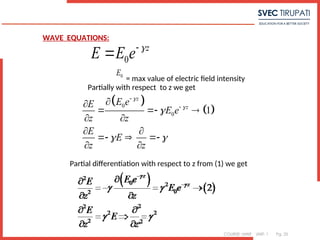
Partially with respect to z we get
= max value of electric field intensity
Partial differentiation with respect to z from (1) we get
WAVE EQUATIONS:
26.
COURSE: MWE UNIT:1 Pg. 26
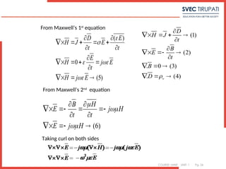
From Maxwell’s 1st
equation
( )
0
(5)
D E
H J E
t t
E
H j E
t
H j E
(1)
(2)
. 0 (3)
. (4)
v
D
H J
t
B
E
t
B
D
From Maxwell’s 2nd
equation
(6)
B H
E j H
t t
E j H
Taking curl on both sides
27.
COURSE: MWE UNIT:1 Pg. 27
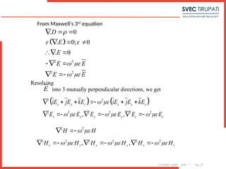
From Maxwell’s 3rd
equation
2 2
2 2
. 0
. 0; 0
. 0
D
E
E
E E
E E
Resolving
E into 3 mutually perpendicular directions, we get
2 2
2 2 2 2 2 2
, ,
x y z x y z
x x y y z z
iE jE kE iE jE kE
E E E E E E
2 2
H H
2 2 2 2 2 2
, ,
x x y y z z
H H H H H H
28.
COURSE: MWE UNIT:1 Pg. 28
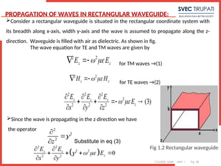
Consider a rectangular waveguide is situated in the rectangular coordinate system with
its breadth along x-axis, width y-axis and the wave is assumed to propagate along the z-
direction. Waveguide is filled with air as dielectric. As shown in fig.
2 2
z z
E E
2 2
z z
H H
The wave equation for TE and TM waves are given by
for TM waves →(1)
for TE waves →(2)
2 2 2
2
2 2 2
(3)
z z z
z
E E E
E
x y z
Since the wave is propagating in the z direction we have
the operator 2
2
2
z
Substitute in eq (3)
2 2
2 2
2 2
0
z z
z
E E
E
x y
PROPAGATION OF WAVES IN RECTANGULAR WAVEGUIDE:
Fig 1.2 Rectangular waveguide
29.
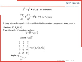
COURSE: MWE UNIT:1 Pg. 29
2 2 2
h
be a constant
2 2
2
2 2
0
z z
z
E E
h E
x y
for TM wave
Using Maxwell’s equation it is possible to find the various components along x and y
directions (Ex
,Ey
,Hx
,Hy
)
From Maxwell’s 1st
equation, we have
H j E
Expand H
x y z
x y z
i j k
j iE iE iE
x y z
H H H
Replacing
z
30.
COURSE: MWE UNIT:1 Pg. 30
x y z
x y z
i j k
j iE iE iE
x y
H H H
,
i j k
Equating coefficients of
4
5
6
z
y x
z
x y
x
z
z
H
H j E
y
H
H j E
x
H
H
j E
x y
Similarly from Maxwell’s 2nd
equation
E j H
31.
COURSE: MWE UNIT:1 Pg. 31
x y z
x y z
i j k
j iH iH iH
x y z
E E E
x y z
x y z
i j k
j iH iH iH
x y
E E E
z
7
8
9
z
y x
z
x y
x
z
z
E
E j H
y
E
E j H
x
E
E
j H
x y
Expanding and equating coefficients
32.
COURSE: MWE UNIT:1 Pg. 32
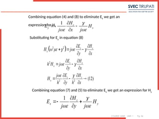
Combining equation (4) and (8) to eliminate Hy
we get an expression for Ex
1 z
y
E Ex
H
j x j x
Substituting for Hy
in equation (4)
2
2
z z
x x
z z
x
H E
E j E
y j x j
H E
E j
j y j x
Multiplying byj
2 2
2 2
z z
x
z z
x
E H
E j
x y
E H
E j
x y
33.
COURSE: MWE UNIT:1 Pg. 33
Where
2 2 2
h
Dividing by –h2
throughout we get
2 2
(10)
z z
x
E H
j
E
h x h y
Combining equation (5) and (7) to eliminate Hy
we get an expression for Ex
1 z
x y
E
H E
j y j
Substituting for Hx
in eq (5)
2 2 z z
y
H E
E j
x y
2 2 2
h
2
2 2
(11)
z z
y
z z
y
H E
h E j
x y
H E
j
E
h x h y
34.
COURSE: MWE UNIT:1 Pg. 34
Combining equation (4) and (8) to eliminate Ey we get an
expression for Hx
1 z
y x
H
E H
j x j
Substituting for Ey
in equation (8)
2 2 z z
x
E H
H j
y x
2
2 2
(12)
z z
x
z z
x
E H
h H j
y x
E H
j
H
h y h x
Combining equation (7) and (5) to eliminate Ex
we get an expression for Hy
1 z
x y
H
E H
j y j
35.
COURSE: MWE UNIT:1 Pg. 35
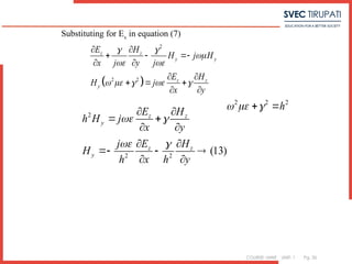
Substituting for Ex
in equation (7)
2
2 2
z z
y y
z z
y
E H
H j H
x j y j
E H
H j
x y
2
2 2
(13)
z z
y
z z
y
E H
h H j
x y
E H
j
H
h x h y
2 2 2
h
36.
COURSE: MWE UNIT:1 Pg. 36
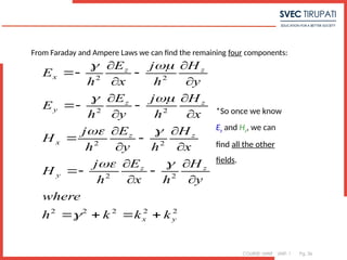
From Faraday and Ampere Laws we can find the remaining four components:
2
2
2
2
2
2
2
2
2
2
2
2
2
y
x
z
z
y
z
z
x
z
z
y
z
z
x
k
k
k
h
where
y
H
h
x
E
h
j
H
x
H
h
y
E
h
j
H
x
H
h
j
y
E
h
E
y
H
h
j
x
E
h
E
*So once we know
Ez and Hz, we can
find all the other
fields.
37.
COURSE: MWE UNIT:1 Pg. 37
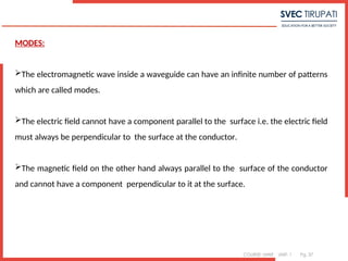
MODES:
The electromagnetic wave inside a waveguide can have an infinite number of patterns
which are called modes.
The electric field cannot have a component parallel to the surface i.e. the electric field
must always be perpendicular to the surface at the conductor.
The magnetic field on the other hand always parallel to the surface of the conductor
and cannot have a component perpendicular to it at the surface.
3
38.
COURSE: MWE UNIT:1 Pg. 38
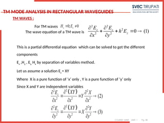
TM MODE ANALYSIS IN RECTANGULAR WAVEGUIDES
For TM waves 0; 0
z z
H E
The wave equation of a TM wave is
2 2
2
2 2
0 (1)
z z
z
E E
h E
x y
This is a partial differential equation which can be solved to get the different
components
Ex
,Hy
, Ey,
Hx
by separation of variables method.
Let us assume a solution Ez
= XY
Where X is a pure function of ‘x’ only , Y is a pure function of ‘y’ only
Since X and Y are independent variables
2
2 2
2 2 2
2
2 2
2 2 2
(2)
(3)
z
z
XY
E X
Y
x x x
XY
E Y
X
y y y
TM WAVES :
39.
COURSE: MWE UNIT:1 Pg. 39
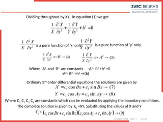
Dividing throughout by XY, in equation (1) we get
2 2
2
2 2
1 1
0
X Y
h
X x Y y
2
2
1 X
X x
is a pure function of ‘x’ only
2
2
1 Y
Y y
is a pure function of ‘y’ only.
2
2
2
1
(4)
X
B
X x
2
2
2
1
(5)
Y
A
Y y
Where -A2
and -B2
are constants -A2
- B2
+h2
=0
-A2
- B2
=h2
→(6)
1 2
3 4
cos sin (7)
cos sin (8)
X c Bx c Bx
Y c Ay c Ay
1 2 3 4
cos sin cos sin (9)
c Bx c Bx c Ay c Ay
Ordinary 2nd
order differential equations the solutions are given by
The complete solution is given by Ez
=XY, Substituting the values of X and Y
Ez
=
Where C1,
C2,
C3,
C4
are constants which can be evaluated by applying the boundary conditions.
40.
COURSE: MWE UNIT:1 Pg. 40
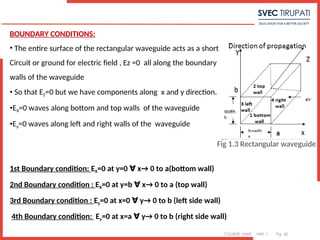
BOUNDARY CONDITIONS:
• The entire surface of the rectangular waveguide acts as a short
Circuit or ground for electric field , Ez =0 all along the boundary
walls of the waveguide
• So that EZ=0 but we have components along x and y direction.
•EX=0 waves along bottom and top walls of the waveguide
•Ey=0 waves along left and right walls of the waveguide
1st Boundary condition: EX=0 at y=0 x→ 0 to a(bottom wall)
∀
2nd Boundary condition : EX=0 at y=b x→ 0 to a (top wall)
∀
3rd Boundary condition : Ey=0 at x=0 y→ 0 to b (left side wall)
∀
4th Boundary condition: Ey=0 at x=a y→ 0 to b (right side wall)
∀
Fig 1.3 Rectangular waveguide
41.
COURSE: MWE UNIT:1 Pg. 41
1 2 3 4
cos sin cos sin
z
E c Bx c Bx c Ay c Ay
1 2 3
1 2
3
0 cos sin
cos sin 0
0
c Bx c Bx c
c Bx c Bx
c
1 2 4
cos sin sin (10)
z
E c Bx c Bx c Ay
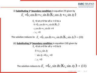
(i) Substituting 1st
boundary condition in equation (9) given by
Ez
=0 at y=0 for all x → 0 to a
The solution reduces to
1 4
4
1
0 sin
sin 0, 0
0
c c Ay
Ay c
c
2 4
sin sin (11)
z
E c Bx c Ay
(ii) Substituting 3rd
boundary condition in equation (10) given by
Ez
=0 at x=0 for all y → 0 to b
The solution reduces to
42.
COURSE: MWE UNIT:1 Pg. 42
2 4
4 2
0 sin sin
sin 0, 0, 0
sin 0
c Bx c Ab
Bx c c
Ab
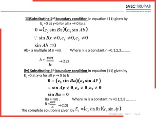
(iii)Substituting 2nd
boundary condition in equation (11) given by
Ez
=0 at y=b for all x → 0 to a
Ab= a multiple of π =nπ Where n is a constant n =0,1,2,3……….
A = →(12)
2 4
sin sin
z
E c Bx c Ay
(iv) Substituting 4th
boundary condition in equation (11) given by
Ez
=0 at x=a for all y → 0 to b
Ba = mπ , Where m is a constant m =0,1,2,3 ………..
B = →(13)
The complete solution is given by
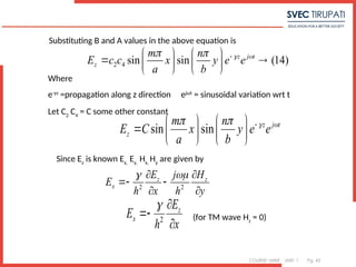
43.
COURSE: MWE UNIT:1 Pg. 43
2 4 sin sin (14)
z j t
z
m n
E c c x y e e
a b
sin sin z j t
z
m n
E C x y e e
a b
Substituting B and A values in the above equation is
Where
e-γz
=propagation along z direction ejωt
= sinusoidal variation wrt t
Let C2
C4
= C some other constant
2 2
z z
x
E H
j
E
h x h y
2
z
x
E
E
h x
Since Ez
is known Ex,
Ey,
Hx,
Hy
are given by
(for TM wave Hz
= 0)
44.
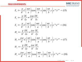
COURSE: MWE UNIT:1 Pg. 44
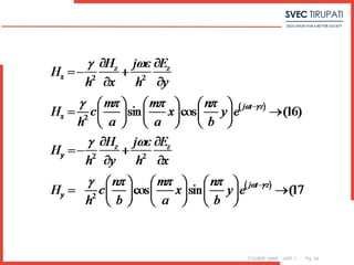
2
2 2
2
2 2
2
(cos sin (15)
(sin cos (16)
(sin cos
z j t
x
z z
y
z j t
y
z z
x
x
m m n
E C x y e e
h a a b
E H
j
E
h y h x
n m n
E C x y e e
h b a b
H E
j
H
h x h y
j n m n
H C x y
h b a b
2 2
2
(17)
(cos sin (18)
z j t
z z
y
z j t
y
e e
H E
j
H
h y h x
j m m n
H C x y e e
h a a b
FIELD COMPONENTS:
45.
COURSE: MWE UNIT:1 Pg. 45
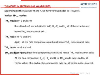
TM MODES IN RECTANGULAR WAVEGUIDES:
Depending on the values of m and n, we have various modes in TM waves.
Various TMmn
modes:
TM00
mode: m= 0 and n =0
If m =0 and n=0 are substituted in Ex
,Hy
, Ey,
and Hx
. all of them vanish and
hence TM00
mode cannot exist.
TM01
mode: m =0 and n=1
Again , all the field components vanish and hence TM01
mode cannot exist.
TM10
mode: m =1 and n=0
Even now , all the field components vanish and hence TM10
mode cannot exist.
TM11
mode: m=1 and n=1
All the four components Ex
,Hy
, Ey,
and Hx
i.e TM11
mode exists and for all
higher values of m and n , the components exist i.e. all higher modes do exist.
46.
COURSE: MWE UNIT:1 Pg. 46
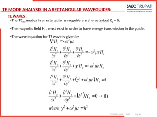
TE MODE ANALYSIS IN A RECTANGULAR WAVEGUIDES:
•The TEmn
modes in a rectangular waveguide are characterized Ez
= 0.
•The magnetic field Hz
, must exist in order to have energy transmission in the guide.
•The wave equation for TE wave is given by
2 2
2 2 2
2
2 2 2
2 2
2 2
2 2
2 2
2 2
2 2
0
z
z z z
z
z z
z z
z z
z
H
H H H
H
x y z
H H
H H
x y
H H
H
x y
2 2
2
2 2
2 2 2
0 (1)
z z
z
H H
h H
x y
where h
TE WAVES :
47.
COURSE: MWE UNIT:1 Pg. 47
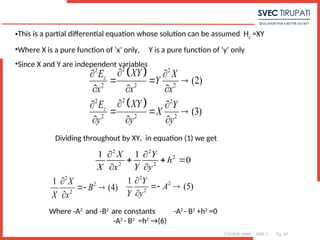
•This is a partial differential equation whose solution can be assumed Hz
=XY
•Where X is a pure function of ‘x’ only, Y is a pure function of ‘y’ only
•Since X and Y are independent variables
2
2 2
2 2 2
2
2 2
2 2 2
(2)
(3)
z
z
XY
E X
Y
x x x
XY
E Y
X
y y y
Dividing throughout by XY, in equation (1) we get
2 2
2
2 2
1 1
0
X Y
h
X x Y y
2
2
2
1
(4)
X
B
X x
2
2
2
1
(5)
Y
A
Y y
Where -A2
and -B2
are constants -A2
- B2
+h2
=0
-A2
- B2
=h2
→(6)
48.
COURSE: MWE UNIT:1 Pg. 48
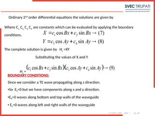
Ordinary 2nd
order differential equations the solutions are given by
1 2
3 4
cos sin (7)
cos sin (8)
X c Bx c Bx
Y c Ay c Ay
Where C1,
C2,
C3,
C4
are constants which can be evaluated by applying the boundary
conditions.
The complete solution is given by Hz
=XY
Substituting the values of X and Y
Hz
=
1 2 3 4
cos sin cos sin (9)
c Bx c Bx c Ay c Ay
BOUNDARY CONDITIONS:
Since we consider a TE wave propagating along z direction.
•So EZ=0 but we have components along x and y direction.
•EX=0 waves along bottom and top walls of the waveguide
• Ey=0 waves along left and right walls of the waveguide
49.
COURSE: MWE UNIT:1 Pg. 49
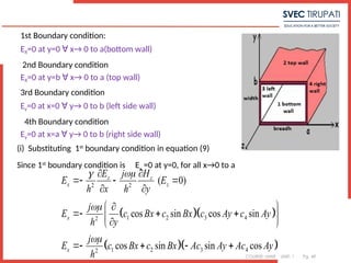
1st Boundary condition:
EX=0 at y=0 x→ 0 to a(bottom wall)
∀
2nd Boundary condition
EX=0 at y=b x→ 0 to a (top wall)
∀
3rd Boundary condition
Ey=0 at x=0 y→ 0 to b (left side wall)
∀
4th Boundary condition
Ey=0 at x=a y→ 0 to b (right side wall)
∀
(i) Substituting 1st
boundary condition in equation (9)
Since 1st
boundary condition is Ex
=0 at y=0, for all x→0 to a
2 2
1 2 3 4
2
1 2 3 4
2
( 0)
cos sin cos sin
cos sin sin cos
z z
x z
x
x
E H
j
E E
h x h y
j
E c Bx c Bx c Ay c Ay
h y
j
E c Bx c Bx Ac Ay Ac Ay
h
50.
COURSE: MWE UNIT:1 Pg. 50
Substituting 1st
boundary condition in the above equation
1 2 4
2
1 2
4
0 cos sin
cos sin 0, 0
0
j
c Bx c Bx Ac
h
c Bx c Bx A
c
The solution reduces to
1 2 3
cos sin cos (10)
z
H c Bx c Bx c Ay
(ii) 3rd
boundary condition
Substituting the 3rd
boundary condition
x =0, y→0 to b
51.
COURSE: MWE UNIT:1 Pg. 51
The solution now reduces to
1 3 cos cos (11)
z
H c c Bx Ay
(iii) 2nd
boundary condition Ez
=0 at y=b, for all x→0 to a
2 2
1 3
2
1 3
2
( 0)
cos cos
cos sin
z z
x z
x
x
E H
j
E E
h x h y
j
E c c Bx Ay
h y
j
E c c A Bx Ay
h
Substituting 2nd
boundary condition
where n=0,1,2,3.......
(12)
Ab n
n
A
b
52.
COURSE: MWE UNIT:1 Pg. 52
(iv) 4th
boundary condition Ey
=0 at x=a, for all y→0 to b
Substituting the boundary condition
The complete solution is 1 3 cos cos
z
H c c Bx Ay
53.
COURSE: MWE UNIT:1 Pg. 53
Substitute for A and B values
1 3
1 3
cos cos
cos cos (13)
z
j t z
z
m n
H c c x y
a b
c c c
m n
H c x y e
a b
FIELD COMPONENTS:
COURSE: MWE UNIT:1 Pg. 55
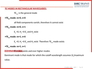
TE MODES IN RECTANGULAR WAVEGUIDES:
TEmn
is the general mode
•TE00
mode: m=0, n=0
all field components vanish, therefore it cannot exist
•TE01
mode: m=0, n=1
Ey
=0, Hx
=0 Ex
and Hy
exist
•TE10
mode: m=1, n=0
Ex
=0, Hy
=0 Ey
and Hx
exist Therefore TE10
mode exists
•TE11
mode: m=1, n=1
This also exists and ever higher modes
DOMINANT MODE:
Dominant mode is that mode for which the cutoff wavelength assumes (λc)maximum
value.
56.
COURSE: MWE UNIT:1 Pg. 56
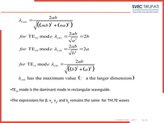
2 2
01 01 2
10 10 2
2
2
TE mod 2
2
TE mod 2
cmn
c
c
ab
mb na
ab
for e b
a
ab
for e a
b
11 01
2 2
10
2
TE mod
has the maximum value a the larger dimension
c
c
ab
for e
b a
•TE10
mode is the dominant mode in rectangular waveguide.
•The expressions for β, vp,
vg
, and λg
remains the same for TM,TE waves
57.
COURSE: MWE UNIT:1 Pg. 57
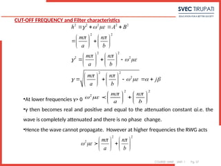
CUT-OFF FREQUENCY and Filter characteristics
•At lower frequencies γ> 0
•γ then becomes real and positive and equal to the attenuation constant αi.e. the
wave is completely attenuated and there is no phase change.
•Hence the wave cannot propagate. However at higher frequencies the RWG acts
2 2 2 2 2
2 2
2 2
2 2
2 2
2
h A B
m n
a b
m n
a b
m n
j
a b
2 2
2 m n
a b
2 2
2 m n
a b
58.
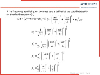
COURSE: MWE UNIT:1 Pg. 58
The frequency at which γ just becomes zero is defined as the cutoff frequency
(or threshold frequency ) fc
.
At f = fc
, γ =0 or ω =2πfc
=ωc
2 2
2
0 c
m n
a b
1
2 2 2
1
2 2 2
1
2 2 2
1
2 2 2
1
1
2
2
2
c
c
c
c
m n
a b
m n
f
a b
c m n
f
a b
c m n
f
a b
59.
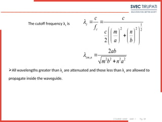
COURSE: MWE UNIT:1 Pg. 59
The cutoff frequency λc is 1
2 2 2
, 2 2 2 2
2
2
c
c
cm n
c c
f
c m n
a b
ab
m b n a
All wavelengths greater than λc
are attenuated and those less than λc
are allowed to
propagate inside the waveguide.
60.
COURSE: MWE UNIT:1 Pg. 60
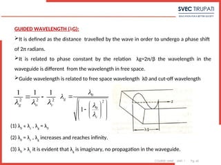
GUIDED WAVELENGTH (λG):
It is defined as the distance travelled by the wave in order to undergo a phase shift
of 2π radians.
It is related to phase constant by the relation λg=2π/β the wavelength in the
waveguide is different from the wavelength in free space.
Guide wavelength is related to free space wavelength λ0 and cut-off wavelength
6
2 2 2
1 1 1
g o c
0
2
0
1
g
c
(1) λ0
« λc
, λg
= λ0
(2) λ0
= λc
, λg
increases and reaches infinity.
(3) λ0
> λc
it is evident that λg
is imaginary, no propagation in the waveguide.
61.
COURSE: MWE UNIT:1 Pg. 61
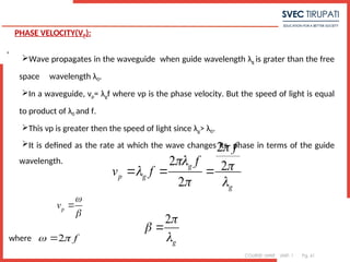
PHASE VELOCITY(VP):
Wave propagates in the waveguide when guide wavelength λg is grater than the free
space wavelength λ0.
In a waveguide, vp= λgf where vp is the phase velocity. But the speed of light is equal
to product of λ0 and f.
This vp is greater then the speed of light since λg> λ0.
It is defined as the rate at which the wave changes its phase in terms of the guide
wavelength.
2
2 2
2
g
p g
g
f
f
v f
p
v
2 f
2
g
where
,
62.
COURSE: MWE UNIT:1 Pg. 62
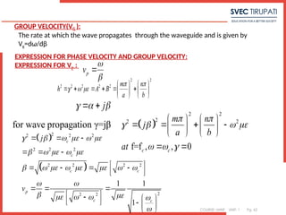
GROUP VELOCITY(VG ):
The rate at which the wave propagates through the waveguide and is given by
Vg=dω/dβ
p
v
2 2
2 2 2 2 2 m n
h A B
a b
j
for wave propagation γ=jβ
2 2
2
2 2
f=f , , 0
c c
m n
j
a b
at
2
2 2 2
2 2 2
2 2 2 2
2
2 2
1 1
1
c
c
c c
p
c c
j
v
EXPRESSION FOR PHASE VELOCITY AND GROUP VELOCITY:
EXPRESSION FOR VP
:
63.
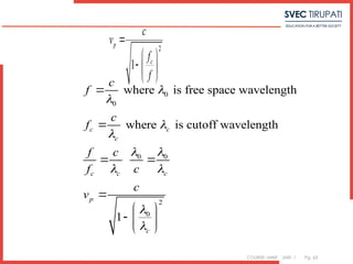
COURSE: MWE UNIT:1 Pg. 63
2
1
p
c
c
v
f
f
0
0
0 0
2
0
where is free space wavelength
where is cutoff wavelength
1
c c
c
c c c
p
c
c
f
c
f
f c
f c
c
v
64.
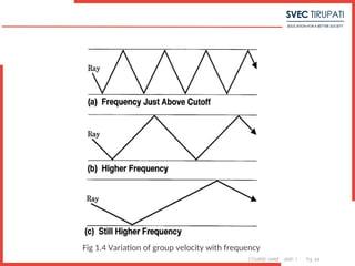
COURSE: MWE UNIT:1 Pg. 64
Fig 1.4 Variation of group velocity with frequency
65.
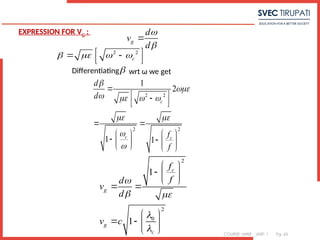
COURSE: MWE UNIT:1 Pg. 65
g
d
v
d
2 2
c
2 2
2 2
1
2
1 1
c
c c
d
d
f
f
2
2
0
1
1
c
g
g
c
f
f
d
v
d
v c
EXPRESSION FOR VG
:
Differentiating wrt ω we get
66.
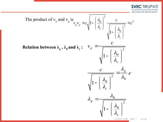
COURSE: MWE UNIT:1 Pg. 66
The product of vp
and vg
is
2
2
0
2
0
1
1
g p
c
c
c
v v c c
Relation between λg
, λ0
and λc
: 2
0
2
0
0
0
2
0
1
.
1
1
p
c
g
c
g
c
c
v
c
c
67.
COURSE: MWE UNIT:1 Pg. 67
2 2
2 2
y
x
z
y x
x y
z
x y
E
E
Z
H H
E E
Z
H H
z
Ex
Hy
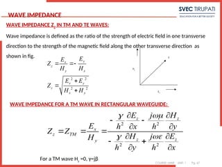
WAVE IMPEDANCE ZZ
IN TM AND TE WAVES:
Wave impedance is defined as the ratio of the strength of electric field in one transverse
direction to the strength of the magnetic field along the other transverse direction as
shown in fig.
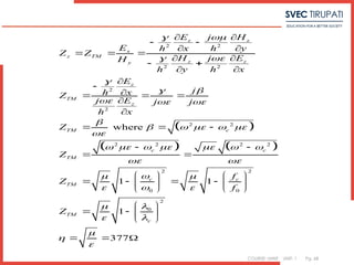
WAVE IMPEDANCE FOR A TM WAVE IN RECTANGULAR WAVEGUIDE:
2 2
2 2
z z
x
z TM
z z
y
E H
j
E h x h y
Z Z
H E
j
H
h y h x
For a TM wave Hz
=0, γ=jβ
WAVE IMPEDANCE
68.
COURSE: MWE UNIT:1 Pg. 68
2 2
2 2
2
2
2 2
2 2 2 2
2 2
0 0
2
0
where
1 1
1
3
z z
x
z TM
z z
y
z
TM
z
TM c
c c
TM
c c
TM
TM
c
E H
j
E h x h y
Z Z
H E
j
H
h y h x
E
j
h x
Z
E
j j j
h x
Z
Z
f
Z
f
Z
77
69.
COURSE: MWE UNIT:1 Pg. 69
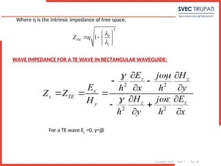
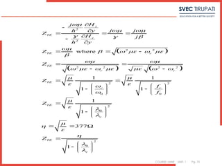
Where η is the intrinsic impedance of free space.
2
0
1
TM
c
Z
WAVE IMPEDANCE FOR A TE WAVE IN RECTANGULAR WAVEGUIDE:
2 2
2 2
z z
x
z TE
z z
y
E H
j
E h x h y
Z Z
H E
j
H
h y h x
For a TE wave Ez
=0, γ=jβ
70.
COURSE: MWE UNIT:1 Pg. 70
2
2
2 2
2 2 2 2
2 2
0 0
2
0
2
0
where
1 1
1 1
1
1
377
1
z
TE
z
TE c
TE
c c
TE
c c
TE
c
TE
c
H
j
j j
h y
Z
H j
h y
Z
Z
Z
f
f
Z
Z
71.
COURSE: MWE UNIT:1 Pg. 71
gair
gdielectric
r
1,
r gdielectric gair
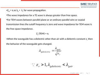
•ZTE
> η as λ0
< λc
for wave propagation.
•The wave impedance for a TE wave is always greater than free space.
•For TEM waves between parallel plane or an ordinary parallel wire or coaxial
transmission lines the cutoff frequency is zero and wave impedance for TEM wave is
the free space impedance.
Zz
(TEM) = η
•When the waveguide has a dielectric other than air with a dielectric constant εr
then
the behavior of the waveguide gets changed.
72.
COURSE: MWE UNIT:1 Pg. 72
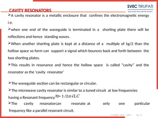
CAVITY RESONATORS
A cavity resonator is a metallic enclosure that confines the electromagnetic energy
i.e.
when one end of the waveguide is terminated in a shorting plate there will be
reflections and hence standing waves.
When another shorting plate is kept at a distance of a multiple of λg/2 than the
hollow space so form can support a signal which bounces back and forth between the
two shorting plates.
This results in resonance and hence the hollow space is called “cavity” and the
resonator as the ‘cavity resonator’
7
The waveguide section can be rectangular or circular.
The microwave cavity resonator is similar to a tuned circuit at low frequencies
having a Resonant frequency f0= 1 /2 √
𝜋 𝐿𝐶
The cavity resonatorcan resonate at only one particular
frequency like a parallel resonant circuit.
73.
COURSE: MWE UNIT:1 Pg. 73
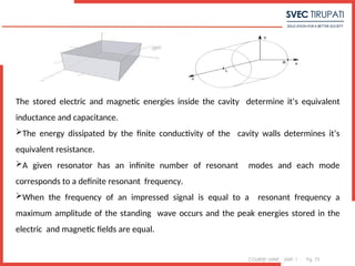
The stored electric and magnetic energies inside the cavity determine it’s equivalent
inductance and capacitance.
The energy dissipated by the finite conductivity of the cavity walls determines it’s
equivalent resistance.
A given resonator has an infinite number of resonant modes and each mode
corresponds to a definite resonant frequency.
When the frequency of an impressed signal is equal to a resonant frequency a
maximum amplitude of the standing wave occurs and the peak energies stored in the
electric and magnetic fields are equal.
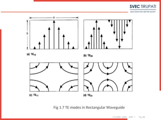
74.
COURSE: MWE UNIT:1 Pg. 74
7
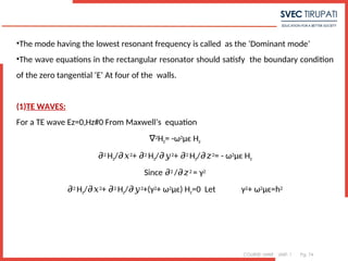
•The mode having the lowest resonant frequency is called as the ‘Dominant mode’
•The wave equations in the rectangular resonator should satisfy the boundary condition
of the zero tangential ‘E’ At four of the walls.
(1)TE WAVES:
For a TE wave Ez=0,Hz#0 From Maxwell’s equation
∇2Hz= -ω2μϵ Hz
𝜕2 Hz/𝜕𝑥2+ 𝜕2 Hz/𝜕𝑦2+ 𝜕2 Hz/𝜕𝑧2= - ω2μϵ Hz
Since 𝜕2 /𝜕𝑧2 = γ2
𝜕2 Hz/𝜕𝑥2+ 𝜕2 Hz/𝜕𝑦2+(γ2+ ω2μϵ) Hz=0 Let γ2+ ω2μϵ=h2
75.
COURSE: MWE UNIT:1 Pg. 75
Let
7
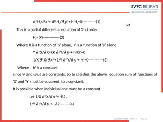
𝜕2 Hz/𝜕𝑥2+ 𝜕2 Hz/𝜕𝑦2+ h2Hz=0-----------(1)
This is a partial differential equation of 2nd order
Hz= XY-------------(2)
Where X is a function of ‘x’ alone, Y is a function of ‘y’ alone
Y 𝜕2 X/𝜕𝑥2+X 𝜕2 Y/𝜕𝑦2+ h2XY=0
1/X 𝜕2 X/𝜕𝑥2+1/Y 𝜕2 Y/𝜕𝑦2+ h2=0------------(3)
Where h2 is a constant
since γ2 and ω2μϵ are constants. So to satisfies the above equation sum of functions of
‘X’ and ‘Y’ must be equalent to a constant.
It is possible when individual one must be a constant.
Let 1/X 𝜕2 X/𝜕𝑥2= -B2 ,
1/Y 𝜕2 Y/𝜕𝑦2= -A2--------(4)
76.
COURSE: MWE UNIT:1 Pg. 76
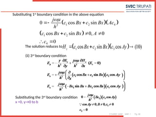
Where A2 and B2 are constants
-A2-B2+ h2=0
h2= A2+B2------------(5)
solutions of equation (4) are X=c1cosBx+c2sinBx------------(6)
Y=c3cosAy+c4sinAy------------(7)
Where c1,c2,c3 and c4 are constants Which are determined by applying boundary
conditions
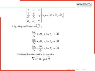
I) BOUNDARY CONDITION(BOTTOM WALL)
Ex=0 for y=0 and all values of x varying from 0 to a we know
Ex= -γ/h2 z/ -jωμ/h
𝜕𝐸 𝜕𝑥 2 z/ Since Ez=0
𝜕𝐻 𝜕𝑦
7
Ex= -jωμ/h2 z/
𝜕𝐻 𝜕𝑦
Ex= -jωμ/h2 / [(c1cosBx + c2sinBx)(c3cosAy+c4sinAy)]
𝜕 𝜕𝑦
= -jωμ/h2[(c2sinBx+c1cosBx)(-Ac3sinAy+Ac4cosAy)]
77.
COURSE: MWE UNIT:1 Pg. 77
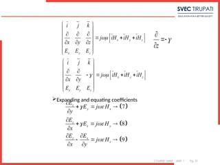
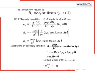
From the boundary condition(i) 0= -jωμ/h2[c1cosBx+c2sinBx]Ac4
[c1cosBx+c2sinBx]Ac4=0 c1cosBx+c2sinBx #0 A#0, c4=0
Hz=( c1cosBx+c2sinBx)(c3cosAy)
Hz= c3(c1cosBx+c2sinBx)cosAy
ii) 2ND BOUNDARY CONDITION[LEFT SIDE WALL] Ey=0 for x=0 and y varying
from 0 to b. Since
Ey= jωμ/h2 𝜕𝐻z/𝜕𝑥
Ey= jωμ/h2 / [(c1cosBx+c2sinBx)c3cosAy]
𝜕 𝜕𝑥
Ey= jωμ/h2[-Bc1sinBx+Bc2cosBx]c3cosAy From the boundary condition
0= jωμ/h2[Bc2c3cosBxcosAy] c3cosAy#0,
c2=0
Hz= c1cosBx.c3cosAy
78.
COURSE: MWE UNIT:1 Pg. 78
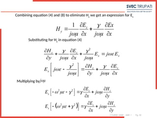
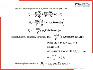
iii)3RD BOUNDARY CONDITION[TOP WALL] Ex=0 for y=b and x varies from 0 to a
Ex= -jωμ/h2 z/
𝜕𝐻 𝜕𝑦
Ex= -jωμ/h2 [ 1 3 ]/
𝜕 𝑐 𝑐 𝑐𝑜𝑠𝐵𝑥𝑐𝑜𝑠𝐴𝑦 𝜕𝑦
= jωμ/h2c1c3AcosBxsinAy c1c3cosBxsinAyb=0
Ab=nπ where n=0,1,2,3----
A=nπ/b
iii) 4TH BOUNDARY CONDITION[RIGHT SIDE WALL] Ey=0 for x=a and y varying from 0
to a Ey= jωμ/h2 / [c1c3cosBxcosAy]
𝜕 𝜕𝑥
= jωμ/h2c1c3BsinBxcosAy
Ey= jωμ/h2c1c3BsinBxcosAy
From the boundary condition Ey=0 for x=a and y varying from 0 to a
c1c3sinBacosAy=0 sinBa=0
Ba=mπ B=mπ/a c1c3=c
Hz= ccos(mπ/a)xcos(nπ/b)ye𝑗(𝜔𝑡−𝛽𝑧)
79.
COURSE: MWE UNIT:1 Pg. 79
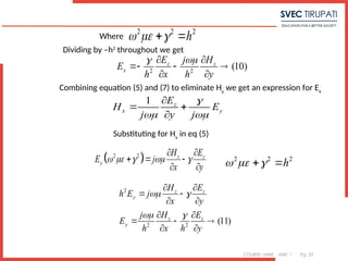
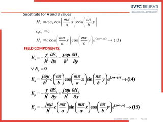
•The amplitude constant along the positive ‘z’ direction is represents by A+ ,and that
along the negative‘z’directionbyA-.
Adding the two travelling waves to obtain the fields of standing wave when we have
from above equation.
Hz= (A+𝑒−𝑗𝛽𝑧+A-𝑒𝑗𝛽𝑧)cos(mπ/a)xcos(nπ/b)y𝑒𝑗𝜔𝑡
To make Ey vanish at z=0 and z=d we must A+= A-
Ey= -γ/h2𝜕𝐸z/ +jωμ/h
𝜕𝑦 2𝜕𝐻z/ since E
𝜕𝑥 z=0
Ey= jωμ/h2 (A
𝜕 + −
𝑒 𝑗𝛽𝑧 + A − 𝑒𝑗𝛽𝑧)cos(mπ/a)xcos(nπ/b)y𝑒𝑗𝜔𝑡]/𝜕𝑥
0= [(A+ −
𝑒 𝑗𝛽𝑧+A-𝑒𝑗𝛽𝑧) − (mπ a )sin(mπ a )xcos(nπ b )y] 𝑒𝑗𝜔𝑡
But sin(mπ a )xcos(nπ b )y#0
Therefore A+ −
𝑒 𝑗𝛽𝑧+A-𝑒𝑗𝛽𝑧 = 0 To make Ey=0, A+= -A-
A+[ −
𝑒 𝑗𝛽𝑧- ]
𝑒𝑗𝛽𝑧 =0 -2jsinβz.A+=0 A+#0 only sinβd=0 with z=d βd=pπ
β=pπ/d
Hz=ccos(mπ/a)xcos(nπ/b)ysin(pπ/d)z𝑒 (
𝑗 − )
𝜔𝑡 𝛽𝑧
80.
COURSE: MWE UNIT:1 Pg. 80
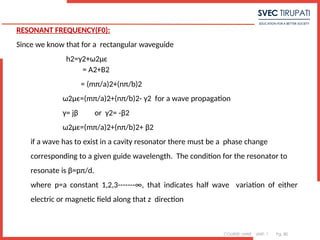
RESONANT FREQUENCY(F0):
Since we know that for a rectangular waveguide
h2=γ2+ω2μϵ
= A2+B2
= (mπ/a)2+(nπ/b)2
ω2μϵ=(mπ/a)2+(nπ/b)2- γ2 for a wave propagation
γ= jβ or γ2= -β2
ω2μϵ=(mπ/a)2+(nπ/b)2+ β2
if a wave has to exist in a cavity resonator there must be a phase change
corresponding to a given guide wavelength. The condition for the resonator to
resonate is β=pπ/d.
where p=a constant 1,2,3-------∞, that indicates half wave variation of either
electric or magnetic field along that z direction
81.
COURSE: MWE UNIT:1 Pg. 81
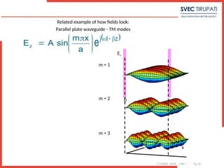
Related example of how fields look:
Parallel plate waveguide - TM modes
a
x
m
sin
A
Ez
z
t
j
e
0 a x
m = 1
m = 2
m = 3
x
z
a
Ez
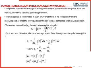
COURSE: MWE UNIT:1 Pg. 85
•The power transmitted through a waveguide and the power loss in the guide walls can
be calculated by a complex poyinting theorem.
•The waveguide is terminated in such away that there is no reflection from the
receiving end or that the waveguide is infinitely long as compared with its wavelength.
•The power transmitted ptr
through a waveguide given by
*
1
.
2
tr
p p ds E H ds
•For a loss less dielectric, the time average power flow through a rectangular waveguide
is
2 2
2
2 2
2
2 2
1
2 2
z
tr
z a a
y
x
z
y x
x y
x y
z
p E da H da
z
E
E
where z
H H
E E E
H H H
POWER TRANSMISSION IN RECTANGULAR WAVEGUIDE:
86.
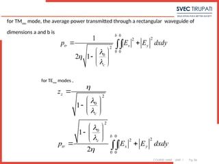
COURSE: MWE UNIT:1 Pg. 86
for TMmn
mode, the average power transmitted through a rectangular waveguide of
dimensions a and b is
0
2
2
2
0 0
0
1
2 1
b
tr x y
c
p E E dxdy
for TEmn
modes ,
2
0
2
0
0
2
2
0 0
1
1
2
z
c
b
c
tr x y
z
p E E dxdy
87.
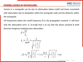
COURSE: MWE UNIT:1 Pg. 87
POWER LOSSES IN WAVEGUIDE:
•Losses in a waveguide can be due to attenuation below cutoff and losses associated
with attenuation due to dissipation within the waveguide walls and the dielectric within
the waveguide.
•At frequencies below the cutoff frequency (f<fc
) the propagation constant ‘γ’ will have
only the attenuation term ‘α’ (γ=α+jβ) that is to say that the phase constant β itself
becomes imaginary implying wave attenuation.
2
2 2
2
cos
1
2
2
1 1
g
g
c
c c c
f
f
f f f
j j j
f c f
88.
COURSE: MWE UNIT:1 Pg. 88
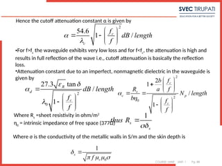
Hence the cutoff attenuation constant α is given by
2
54.6
1 /
c
c
f
dB length
f
•For f>fc
the waveguide exhibits very low loss and for f<fc
, the attenuation is high and
results in full reflection of the wave i.e., cutoff attenuation is basically the reflection
loss.
•Attenuation constant due to an imperfect, nonmagnetic dielectric in the waveguide is
given by
2
0
27.3 tan
/
1
R
d
c
dB length
f
f
2
2
0
2
1
/
1
c
s
c p
c
f
b
a f
R
N length
b f
f
Where Rs
=sheet resistivity in ohm/m2
η0
= intrinsic impedance of free space (377Ω)
1
s
s
thus R
Where σ is the conductivity of the metallic walls in S/m and the skin depth is
0
1
s
r
f
89.
COURSE: MWE UNIT:1 Pg. 89
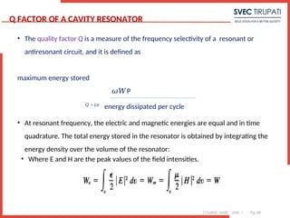
• The quality factor Q is a measure of the frequency selectivity of a resonant or
antiresonant circuit, and it is defined as
maximum energy stored
𝜔𝑊P
𝑄 = 2𝜋
energy dissipated per cycle
• At resonant frequency, the electric and magnetic energies are equal and in time
quadrature. The total energy stored in the resonator is obtained by integrating the
energy density over the volume of the resonator:
Q FACTOR OF A CAVITY RESONATOR
• Where E and H are the peak values of the field intensities.
90.
COURSE: MWE UNIT:1 Pg. 90
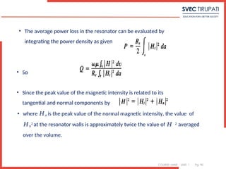
• The average power loss in the resonator can be evaluated by
integrating the power density as given
• So
• Since the peak value of the magnetic intensity is related to its
tangential and normal components by
• where 𝐻𝑛 is the peak value of the normal magnetic intensity, the value of
𝐻𝑛
2 at the resonator walls is approximately twice the value of 𝐻 2 averaged
over the volume.
91.
COURSE: MWE UNIT:1 Pg. 91
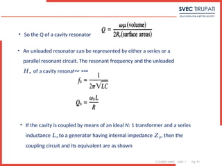
• So the Q of a cavity resonator
• An unloaded resonator can be represented by either a series or a
parallel resonant circuit. The resonant frequency and the unloaded
𝐻𝑛 of a cavity resonator are
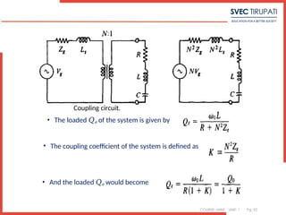
• If the cavity is coupled by means of an ideal N: 1 transformer and a series
inductance 𝐿𝑠 to a generator having internal impedance 𝑍𝑔, then the
coupling circuit and its equivalent are as shown
92.
COURSE: MWE UNIT:1 Pg. 92
Coupling circuit.
• The loaded 𝑄𝑒 of the system is given by
• The coupling coefficient of the system is defined as
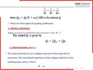
• And the loaded 𝑄𝑒 would become
93.
COURSE: MWE UNIT:1 Pg. 93
• There are three types of coupling coefficients:
1. CRITICAL COUPLING:
If the resonator is matched to the generator, then = 1
𝐾
2. OVER COUPLING: IF K > 1
• The cavity terminals are at a voltage maximum in the input line at
resonance. The normalized impedance at the voltage maximum is the
standing-wave ratio 𝜌. That is
𝐾 = 𝜌
94.
COURSE: MWE UNIT:1 Pg. 94
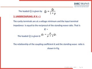
The loaded 𝑄𝑙 is given by
3. UNDERCOUPLING: IF K < 1
The cavity terminals are at a voltage minimum and the input terminal
impedance is equal to the reciprocal of the standing-wave ratio. That is
1/𝞺
𝐾 =
The loaded 𝑄𝑙 is given by
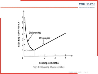
The relationship of the coupling coefficient K and the standing-wave ratio is
shown in Fig.
COURSE: MWE UNIT:1 Pg. 96
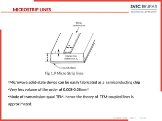
MICROSTRIP LINES
•Microwave solid-state device can be easily fabricated as a semiconducting chip
•Very less volume of the order of 0.008-0.08mm3
•Mode of transmission-quasi TEM, hence the theory of TEM-coupled lines is
approximated.
Fig 1.9 Micro Strip lines
97.
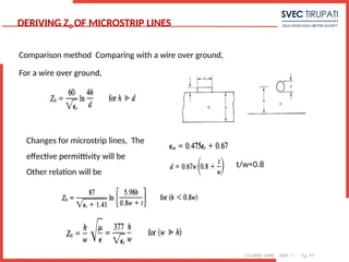
COURSE: MWE UNIT:1 Pg. 97
DERIVING ZO OF MICROSTRIP LINES
Comparison method Comparing with a wire over ground,
For a wire over ground,
Changes for microstrip lines, The
effective permittivity will be
Other relation will be
t/w<0.8
98.
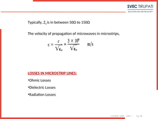
COURSE: MWE UNIT:1 Pg. 98
Typically, Zo is in between 50Ω to 150Ω
The velocity of propagation of microwaves in microstrips,
LOSSES IN MICROSTRIP LINES:
•Ohmic Losses
•Dielectric Losses
•Radiation Losses
99.
COURSE: MWE UNIT:1 Pg. 99
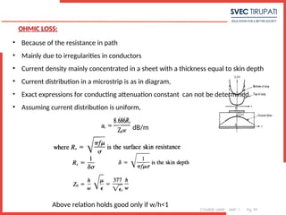
OHMIC LOSS:
• Because of the resistance in path
• Mainly due to irregularities in conductors
• Current density mainly concentrated in a sheet with a thickness equal to skin depth
• Current distribution in a microstrip is as in diagram,
• Exact expressions for conducting attenuation constant can not be determined.
• Assuming current distribution is uniform,
dB/m
Above relation holds good only if w/h<1
100.
COURSE: MWE UNIT:1 Pg. 100
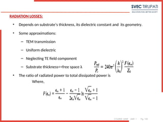
RADIATION LOSSES:
• Depends on substrate’s thickness, its dielectric constant and its geometry.
• Some approximations:
– TEM transmission
– Uniform dielectric
– Neglecting TE field component
– Substrate thickness<<free space λ
• The ratio of radiated power to total dissipated power is
Where,
101.
COURSE: MWE UNIT:1 Pg. 101
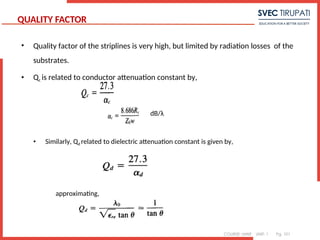
QUALITY FACTOR
• Quality factor of the striplines is very high, but limited by radiation losses of the
substrates.
• Qc is related to conductor attenuation constant by,
dB/λ
• Similarly, Qd related to dielectric attenuation constant is given by,
approximating,
102.
COURSE: MWE UNIT:1 Pg. 102
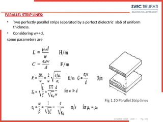
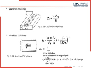
PARALLEL STRIP LINES:
• Two perfectly parallel strips separated by a perfect dielectric slab of uniform
thickness.
• Considering w>>d,
some parameters are
Fig 1.10 Parallel Strip lines
103.
COURSE: MWE UNIT:1 Pg. 103
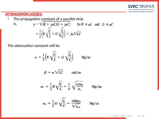
ATTENUATION LOSSES:
• The propagation constant of a parallel strip
is,
The attenuation constant will be


![COURSE: MWE UNIT: 1 Pg. 76
Where A2 and B2 are constants
-A2-B2+ h2=0
h2= A2+B2------------(5)
solutions of equation (4) are X=c1cosBx+c2sinBx------------(6)
Y=c3cosAy+c4sinAy------------(7)
Where c1,c2,c3 and c4 are constants Which are determined by applying boundary
conditions
I) BOUNDARY CONDITION(BOTTOM WALL)
Ex=0 for y=0 and all values of x varying from 0 to a we know
Ex= -γ/h2 z/ -jωμ/h
𝜕𝐸 𝜕𝑥 2 z/ Since Ez=0
𝜕𝐻 𝜕𝑦
7
Ex= -jωμ/h2 z/
𝜕𝐻 𝜕𝑦
Ex= -jωμ/h2 / [(c1cosBx + c2sinBx)(c3cosAy+c4sinAy)]
𝜕 𝜕𝑦
= -jωμ/h2[(c2sinBx+c1cosBx)(-Ac3sinAy+Ac4cosAy)]](https://image.slidesharecdn.com/iiiecemweuniti-250419064820-588fe3d5/85/III-ECE-MWE-UNIT-i-types-of-waveguides-analysis-76-320.jpg)
![COURSE: MWE UNIT: 1 Pg. 77
From the boundary condition(i) 0= -jωμ/h2[c1cosBx+c2sinBx]Ac4
[c1cosBx+c2sinBx]Ac4=0 c1cosBx+c2sinBx #0 A#0, c4=0
Hz=( c1cosBx+c2sinBx)(c3cosAy)
Hz= c3(c1cosBx+c2sinBx)cosAy
ii) 2ND BOUNDARY CONDITION[LEFT SIDE WALL] Ey=0 for x=0 and y varying
from 0 to b. Since
Ey= jωμ/h2 𝜕𝐻z/𝜕𝑥
Ey= jωμ/h2 / [(c1cosBx+c2sinBx)c3cosAy]
𝜕 𝜕𝑥
Ey= jωμ/h2[-Bc1sinBx+Bc2cosBx]c3cosAy From the boundary condition
0= jωμ/h2[Bc2c3cosBxcosAy] c3cosAy#0,
c2=0
Hz= c1cosBx.c3cosAy](https://image.slidesharecdn.com/iiiecemweuniti-250419064820-588fe3d5/85/III-ECE-MWE-UNIT-i-types-of-waveguides-analysis-77-320.jpg)
![COURSE: MWE UNIT: 1 Pg. 78
iii)3RD BOUNDARY CONDITION[TOP WALL] Ex=0 for y=b and x varies from 0 to a
Ex= -jωμ/h2 z/
𝜕𝐻 𝜕𝑦
Ex= -jωμ/h2 [ 1 3 ]/
𝜕 𝑐 𝑐 𝑐𝑜𝑠𝐵𝑥𝑐𝑜𝑠𝐴𝑦 𝜕𝑦
= jωμ/h2c1c3AcosBxsinAy c1c3cosBxsinAyb=0
Ab=nπ where n=0,1,2,3----
A=nπ/b
iii) 4TH BOUNDARY CONDITION[RIGHT SIDE WALL] Ey=0 for x=a and y varying from 0
to a Ey= jωμ/h2 / [c1c3cosBxcosAy]
𝜕 𝜕𝑥
= jωμ/h2c1c3BsinBxcosAy
Ey= jωμ/h2c1c3BsinBxcosAy
From the boundary condition Ey=0 for x=a and y varying from 0 to a
c1c3sinBacosAy=0 sinBa=0
Ba=mπ B=mπ/a c1c3=c
Hz= ccos(mπ/a)xcos(nπ/b)ye𝑗(𝜔𝑡−𝛽𝑧)](https://image.slidesharecdn.com/iiiecemweuniti-250419064820-588fe3d5/85/III-ECE-MWE-UNIT-i-types-of-waveguides-analysis-78-320.jpg)
![COURSE: MWE UNIT: 1 Pg. 79
•The amplitude constant along the positive ‘z’ direction is represents by A+ ,and that
along the negative‘z’directionbyA-.
Adding the two travelling waves to obtain the fields of standing wave when we have
from above equation.
Hz= (A+𝑒−𝑗𝛽𝑧+A-𝑒𝑗𝛽𝑧)cos(mπ/a)xcos(nπ/b)y𝑒𝑗𝜔𝑡
To make Ey vanish at z=0 and z=d we must A+= A-
Ey= -γ/h2𝜕𝐸z/ +jωμ/h
𝜕𝑦 2𝜕𝐻z/ since E
𝜕𝑥 z=0
Ey= jωμ/h2 (A
𝜕 + −
𝑒 𝑗𝛽𝑧 + A − 𝑒𝑗𝛽𝑧)cos(mπ/a)xcos(nπ/b)y𝑒𝑗𝜔𝑡]/𝜕𝑥
0= [(A+ −
𝑒 𝑗𝛽𝑧+A-𝑒𝑗𝛽𝑧) − (mπ a )sin(mπ a )xcos(nπ b )y] 𝑒𝑗𝜔𝑡
But sin(mπ a )xcos(nπ b )y#0
Therefore A+ −
𝑒 𝑗𝛽𝑧+A-𝑒𝑗𝛽𝑧 = 0 To make Ey=0, A+= -A-
A+[ −
𝑒 𝑗𝛽𝑧- ]
𝑒𝑗𝛽𝑧 =0 -2jsinβz.A+=0 A+#0 only sinβd=0 with z=d βd=pπ
β=pπ/d
Hz=ccos(mπ/a)xcos(nπ/b)ysin(pπ/d)z𝑒 (
𝑗 − )
𝜔𝑡 𝛽𝑧](https://image.slidesharecdn.com/iiiecemweuniti-250419064820-588fe3d5/85/III-ECE-MWE-UNIT-i-types-of-waveguides-analysis-79-320.jpg)