This document describes an analysis of the design constraints and weight estimation for an electric propeller-driven RC aircraft. It outlines the development of computer programs to model the aircraft's performance based on input parameters, calculate required power-to-weight ratios for different flight phases, and estimate take-off weight based on battery weight. The programs analyze how wing loading and power-to-weight ratio are related given performance requirements, and compute the battery, payload, and empty weights needed to meet those requirements.

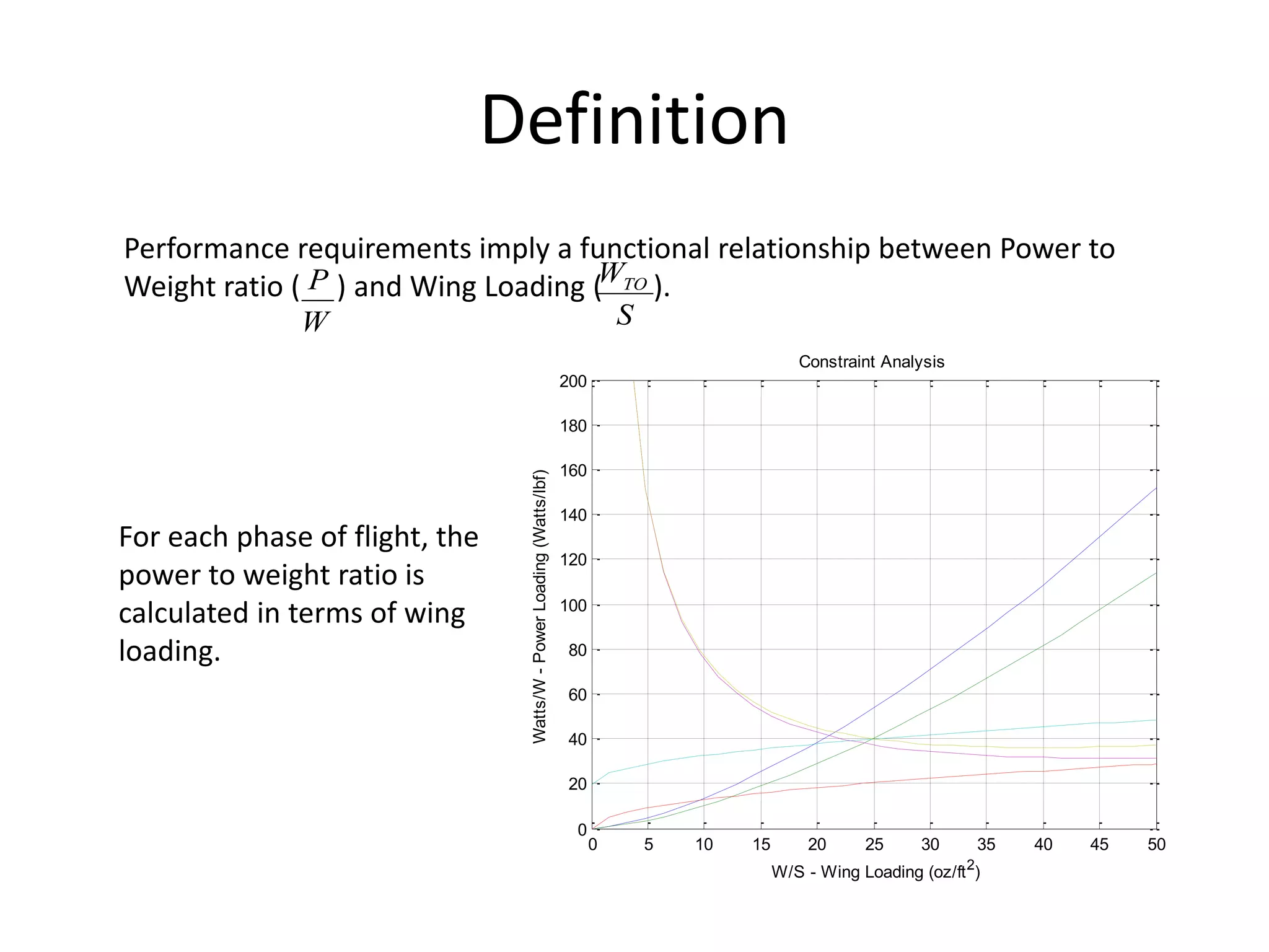
1. Electric Propeller Driven RC Aircraft
Constraint Analysis/Weight Estimation/Flight Simulation/Optimization
Purdue University
AIAA Design Build Fly Team
2007-2008

2. Battery Motor
Propeller
m

p

p
m
elec
elec
m
shaf t
p
available
required
opeller
Pr
Tv
P
P
Tv
P
Tv
Power
Power
Efficiency










batt
batt
W
E
K 
prop
motor
overall 

 
Electric Propulsion Model
Measures of efficiency:
batt
K
Battery Energy Density:

3. CONSTRAINT ANALYSIS
Quantifying the target design space

4. Definition
Performance requirements imply a functional relationship between Power to
Weight ratio ( ) and Wing Loading ( ).
W
P
S
WTO
0 5 10 15 20 25 30 35 40 45 50
0
20
40
60
80
100
120
140
160
180
200
Constraint Analysis
W/S - Wing Loading (oz/ft2
)
Watts/W
-
Power
Loading
(Watts/lbf)
For each phase of flight, the
power to weight ratio is
calculated in terms of wing
loading.

5. Code Structure
input.dat
(can rename as required)
constraint.m
(Run this file to run code)
Turns
Turns
Max
Speed
Rate of
Climb
Ceiling
Landing
Takeoff
Calculate
C_D, K, L/D

6. Aircraft Input Parameters
The following parameters must be estimated based on the type of aircraft and
past experience.
Aspect Ratio
Span Efficiency Factor
Zero Lift Drag
The drag for any condition is:
2
L
D
D KC
C
C o


)
/(
1 e
AR
K 

 
The maximum lift/drag ratio is
o
D
MAX
MAX
KC
2
1
E
)
D
/
L
( 

A sample input is provided below. This is representative of a typical conventional
aircraft.
Computer Program Input
aircraft (This must be the first line)
5.0 Aspect ratio (AR)
0.8 Span Efficiency (e)

7. Takeoff
From Brandt et. al. Equation 5.52, the takeoff velocity is found by:
Stall
TO
L
SL
TO
Stall
V
V
C
S
W
V
MAX



2
.
1
2

The Power/Weight (Watts/lbf) ratio is given by:
 
gd
V
W
P
m
p
TO


*
550
*
2
7
.
0
/
3


Computer Program Input
Takeoff
500. Altitude (ft)
1.5 Cl_max
75. Take off distance (ft)
Note: Velocity taken to be mean velocity till
take-off (=70% of take-off velocity)
(Brandt Eqs 5.52 and 5.77)

8. Landing
The take off velocity is again calculated:
MAX
L
SL
TO
TO
C
S
W
V

2
2
.
1

The Power/Weight (Watts/lbf) ratio is given by:
gd
V
W
P
m
p
TO


550
/
3

Computer Input
Landing
500. altitude (ft)
1.5 MAX
L
C
100 landing distance
(Brandt Eqs 5.52 and 5.77)

9. Ceiling
The Coefficient of lift (at minimum drag/velocity) is given as:
k
C
C do
l
3

l
To
y
C
S
W
V

2

The Power/Weight ratio is given by:


 g
V
W
P
m
p
y
*
550
*
866
.
/ 
Computer Input
Ceiling
500. Altitude (ft)

10. Rate of Climb
The Coefficient of lift (at minimum drag/velocity) is given as:
k
C
C do
l
3

l
To
power
C
S
W
V

2
min 
The Power/Weight ratio is given by:
  




















max
min
866
.
*
550
1
/
D
L
V
RofC
W
P
power
m
p
Computer Input
Ceiling
500. Altitude (ft)

11. Maximum Speed
By definition, the dynamic pressure is:
2
2
1
V
q 

The thrust to weight ratio is calculated by the equation:
)
)(
1
(
q
S
W
k
S
W
qC
W
T
TO
TO
do



The power to weight ratio is:
m
p
W
T
V
W
P


*
550
)
(
/ 
Computer Input
max speed
500. Altitude (ft)
100 Airspeed (ft/s)

12. Turn
The Power/Weight ratio for turns is determined the same way as that of the
Maximum Speed function but with a load factor (dependent on bank angle) in
the thrust-to-weight ratio equation.
2
2
1
V
q 

)
)(
1
( 2
q
S
W
k
n
S
W
qC
W
T
To
To
do



m
p
W
T
V
W
P


*
550
/ 
Computer Input
turn
35000. Altitude (ft)
660. airspeed (ft/sec)
1.15 load factor – n

13. Running the Constraint Program
• Download and unzip the constraint analysis code(s) from Team Center.
• In the folder, you will see a program called constraint.m. This is the
master program, and it calls all of the other .m files as functions.
– There is no need to edit the master program, but feel free to take a look at the
program and its functions to understand how it works.
– Run constraint.m in MATLAB, it will prompt you for an input file
(contraint_input.dat).
– Desired constraints can be analyzed by updating the aircraft parameters and
flight segments in the input file (contraint_input.dat).
• The program will output (to the MATLAB command screen) some various
values (mostly the data you have input). If you wish to see additional
numerical data, feel free to change the program to print out the data.
• A graph of Wing Loading (oz/ft2) vs. Power to Weight Ratio (Watts/lbf) will
be created, showing the energy required for each of the legs of the
mission. An example of the output follows.

14. The input file is called contraint_input.dat (You can rename it to whatever you
want). Here is an example set of inputs:
airplane
5.00 aspect ratio
0.08 Cdo
0.60 propellor efficiency
0.60 motor efficiency
0.80 oswald efficiciency
take off
1300. altitude (ft)
1.2 Clmax
75. takeoff distance (ft)
landing
1300. altitude (ft)
1.2 Clmax
100. landing distance (ft)
0. reverse force fraction
ceiling
1400. altitude (ft)
rate-of-climb
1400. altitude (ft)
5. R/C (ft/sec)
max speed
1400. altitude (ft)
42. airspeed (ft/sec)
turn
1400. altitude (ft)
50. airspeed (ft/sec)
1.15 load factor
•Each of the numbers in the input
file must have a decimal in it. For
example, 1.2, or 75. (not 75).
•Do not change the order of the
different variables. Don’t change
anything but the numbers!
•The altitude is MSL (Altitude
above Mean Sea Level).
•You can repeat certain legs, for
example, you can have multiple
turn segments, ceilings, etc. To do
so, simply add the new flight
profiles to the input file. Sequence
of flight segments is not important.
Mission
Legs
Edit as
required
Edit as required

15. Sample Output
0 10 20 30 40 50 60 70
0
20
40
60
80
100
120
140
160
180
200
Constraint Analysis
W/S - Wing Loading (oz/ft2
)
Watts/W
-
Specific
Power
(Watts/lbf)
Takeoff
Landing
Ceiling
R of C
Max Vel
Turn

16. WEIGHT ANALYSIS
Estimating aircraft weight/size

17. Rearrange terms












TO
B
TO
E
PL
TO
W
W
W
W
W
W
1
Take-off
Weight
Empty
Weight
Payload
Weight
Battery Weight
for each flight leg



 B
PL
E
TO W
W
W
W
Mission Input
Empirically
Derived
Mission
Output
Computed for
each flight leg
Take-Off Weight Computation

18. SLUF Battery Weight Fraction
)
D
/
L
(
K
x
W
W
P
W
K
W
)
D
/
L
(
P
vt
x
dt
dx
v
P
W
K
t
W
t
P
K
W
)
D
/
L
(
P
v
W
L
D
D
...
but
...
D
P
v
P
Dv
P
Tv
Power
Power
D
T
_
_&
W
L
SLUF
batt
p
m
TO
B
elec
B
batt
TO
p
m
elec
elec
B
batt
B
elec
batt
TO
p
m
elec
TO
p
m
elec
elec
m
Shaft
Actual
quired
Re
p
TO





























Brandt p42

19. Flight Segments
 c
batt
m
p
C
TO
B
D
/
L
k
x
W
W



 
max
L
TO
stall
LO
C
S
/
W
2
2
.
1
v
2
.
1
v




 
)
W
/
P
(
g
v
7
.
0
x
TO
m
p
3
LO
TO




 
o
D
TO
BR
C
k
S
/
W
2
v


Take-off:
Cruise (Type 1 – Best Range; Type 2 – Velocity Specified)
Sustained Turn:
2
L
D
D kC
C
C o

  
o
D
max
C
AR
e
2
1
D
/
L




Aerodynamic Model:
 L
batt
m
p
L
TO
B
D
/
L
k
x
W
W



 
o
D
TO
L
C
3
k
S
/
W
2
v


Loiter (Max. Endurance)
 max
L D
/
L
866
.
0
)
D
/
L
( 
   






 




S
/
W
C
q
v
)
W
/
P
(
S
/
W
k
q
n
TO
D
m
p
TO
TO
o
AR
e
1
k




1
n
g
k
v
)
W
/
P
(
2
W
W
2
batt
T
TO
TO
B



Reference: Aircraft Design: A Conceptual Approach, Daniel P. Raymer
q
)
S
/
W
(
k
q
C
)
S
/
W
(
)
D
/
L
( 2
TO
Do
TO
c



20. Assumptions
• The weight fraction is known and achievable
– 0.23 for most competitive AIAA D/B/F aircraft
– 0.40 for AIAA D/B/F competition average
• The motor and propeller efficiencies are constant (not true!)
• Known 2 term aircraft aerodynamic drag model is applicable
– Estimate and update based on wind-tunnel testing
• Wind speeds/directions not considered
– Increased power requirement for upwind flight segments with a headwind are
not offset by reduced power requirements on the downwind flight segment.
• Human-in-the-loop – Pilot cannot always operate aircraft at optimal
design point!
– Safety factor required to achieve design performance specification

21. Running the Weight Program
• Download and unzip the constraint analysis code(s) from Team Center.
• In the folder, you will see a program called weight.m. This is the master
program, and it calls all of the other .m files as functions.
– There is no need to edit the master program, but feel free to take a look at the
program and its functions to understand how it works.
– Update to input file (weight_input.txt) to include desired aircraft parameters
and define different flight segments.
– Run weight.m in MATLAB, it will prompt you for an input file
(weight_input.txt).
• Aircraft weight break-up and performance summary for each flight leg will
be output to the Matlab screen. An example of the output follows.

22. The input file is called weight_input.dat (You can rename it to whatever you want).
Here is an example set of inputs:
airplane
5. aspect ratio
0.08 Cdo
0.65 span efficiency
0.60 propeller efficiency
0.60 motor efficiency
22. wing loading (oz weight/ft2)
45. power to weight (Watt/lbf)
70000. energy (Joules) / Battery Weight (lbf)
0.40 empty weight fraction (emperical)
7.2 payload weight (lbf)
take-off
1300. altitude (ft)
1.2 Clmax
climb
100 alitude above ground to climb to (ft)
1. delta (% of max power)
c1
1400. altitude (ft)
7000. cruise distance (ft)
c2
1400. altitude (ft)
7000. cruise distance (ft)
40. cruise velocity (ft/s)
lo
1400. altitude (ft)
7000. cruise distance (ft)
t1
1400. altitude (ft)
720. turn angle (degrees)
1.8 clmax
t2
1400. altitude (ft)
31.05 turn velocity (ft/s)
720. turn angle (degrees)
•Each of the numbers in the input
file must have a decimal in it. For
example, 1.2, or 75. (not 75).
•Do not change the order of the
different variables. Don’t change
anything but the numbers!
•The altitude is MSL (Altitude
above Mean Sea Level).
•You can repeat certain legs, for
example, you can have multiple
turn segments, ceilings, etc. To do
so, simply add the new flight
profiles to the input file. Sequence
of flight segments is not important.
Mission
Legs
Edit as
required
Edit as required
Note: Climb module available, but current version
requires improvement and is not recommended for use.

23. Sample Output

24. FLIGHT ANALYSIS
Estimating aircraft performance

25. Running the Flight Program
• Download and unzip the constraint analysis code(s) from Team Center.
• In the folder, you will see a program called flight.m. This is the master
program, and it calls all of the other .m files as functions.
– There is no need to edit the master program, but feel free to take a look at the
program and its functions to understand how it works.
– Update to input file (flight_input.txt) to include desired aircraft parameters
and define different flight segments.
– Run flight.m in MATLAB, it will prompt you for an input file (flight_input.txt).
• Aircraft performance summary for each flight leg will be output to the
Matlab screen, including energy requirements and surplus. An example of
the output follows.

26. The input file is called flight_input.dat (You can rename it to whatever you want).
Here is an example set of inputs:
airplane
5. aspect ratio
0.08 Cdo
0.65 span efficiency
0.60 propeller efficiency
0.60 motor efficiency
70000. Energy (Joules) / Battery Weight (lbf)
7.2 payload weight (lbf)
7.96 empty weight (lbf)
4.75 battery weight
14.48 wing planform area (ft^2)
895.95 motor power (watts)
take-off
1300. altitude (ft)
1.2 Clmax
climb
100 alitude above ground to climb to (ft)
1. delta (% of max power)
c1
1400. altitude (ft)
7000. cruise distance (ft)
c2
1400. altitude (ft)
7000. cruise distance (ft)
40. cruise velocity (ft/s)
lo
1400. altitude (ft)
7000. cruise distance (ft)
t1
1400. altitude (ft)
720. turn angle (degrees)
1.8 clmax
t2
1400. altitude (ft)
31.05 turn velocity (ft/s)
720. turn angle (degrees)
•Each of the numbers in the input
file must have a decimal in it. For
example, 1.2, or 75. (not 75).
•Do not change the order of the
different variables. Don’t change
anything but the numbers!
•The altitude is MSL (Altitude
above Mean Sea Level).
•You can repeat certain legs, for
example, you can have multiple
turn segments, ceilings, etc. To do
so, simply add the new flight
profiles to the input file. Sequence
of flight segments is not important.
Mission
Legs
Edit as
required
Edit as required
Note: Climb module available, but current version
requires improvement and is not recommended for use.

27. Sample Output

28. PERFORMACE OPTIMIZER
Iterating through the feasible design space

29. Program Format
• Software Platform: Matlab
• Flight Profiles: mission1.m, mission2.m
– Specify flight segment types, distances, etc. for
each flight mission
• Main program: optimize.m
– Define design space, aircraft constants and scoring
parameters
• Program Output: Matlab screen
– No output file

30. Mission Profiles (missionx.m)
• Place blue text in mission files in any sequence and any number of times. Required
inputs are placed in <> and outputs include flight segment name (leg(i,:)), battery
weight fraction (wb_wto(i,:)), velocity (v(i,:)) in ft/s, time (t(i,:)) in seconds and
distance (x(i,:)) in feet. Input units are feet and degrees.
• Take-off:
[leg(i,:) wb_wto(i,:) v(i,:) t(i,:) x(i,:)]=takeoffp((<altitude>, <Clmax>)
• Straight & Level Flight
– Cruise Type 1 (Min. Power Consumption)
[leg(i,:) wb_wto(i,:) v(i,:) t(i,:) x(i,:)]=cruise1p(<altitude>, <distance>);
– Cruise Type 2 (Specified Velocity)
[leg(i,:) wb_wto(i,:) v(i,:) t(i,:) x(i,:)]=cruise2p(<altitude>, <distance>, <velocity>);
– Loiter (Max. Endurance)
[leg(i,:) wb_wto(i,:) v(i,:) t(i,:) x(i,:)]=loiterp(<altitude>, <distance>);
• Turns
– Turn Type 1 (Min. Power Consumption)
[leg(i,:) wb_wto(i,:) v(i,:) t(i,:) x(i,:)]=turn1p(<altitude>, <angle>);
– Turn Type 2 (Velocity Specified)
[leg(i,:) wb_wto(i,:) v(i,:) t(i,:) x(i,:)]=turn1p(<altitude>, <velocity>, <angle>);
Note: Climb module available, but current version requires improvement and is not recommended for use.

31. Main Program (optimize.m)
• Input aircraft parameters
• Establish mission constraint to obtain required specific power
requirements
– Usually take-off distance requirement
• Size aircraft for heaviest payload mission
• Evaluate aircraft performance for other missions
• Iterate through wing loadings and aspect ratios to optimize
parameters of interest!
• File provided is based on 2007-2008 competition and will
require to be tailored for each year’s requirements.

32. Example: 2007-2008 Flowchart
INPUT:
Wing Loading (WTO/S) &
Aspect Ratio (AR)
MAIN PROGRAM LOOP
Drag
Coefficient:
Take-off
Weight:
TAKE-OFF
Take-off
Velocity:
Take-off
Distance:
PAYLOAD MISSION T/O WEIGHT












2
TO
2
B
TO
E
2
PL
2
TO
W
W
W
W
1
W
W



 B
PL
E
TO W
W
W
W
)
AR
(
e
C
C
C
2
L
D
D o



 
max
L
TO
LO
C
S
/
W
2
2
.
1
v


 
)
W
/
P
(
g
v
7
.
0
x
TO
m
p
3
LO
TO




CRUISE
Min. Power
Cruise Point:
Battery Weight
Fraction:
TURN
Iterate load factor (n) and turn velocity.
Minimize Battery Weight Fraction:
 max
batt
p
p
cruise
TO
B
D
/
L
k
x
W
W



 
 











)
AR
(
e
q
S
/
W
n
S
/
W
q
C
k
x
W
W TO
2
TO
D
batt
p
p
turn
TO
B o
 
o
D
max
C
)
AR
(
e
1
2
1
D
/
L


EMPTY MISSION T/O WEIGHT











1
TO
1
B
E
1
TO
W
W
1
W
W
MISSION 2 SCORE
MISSION 1 SCORE
2
B
E
loading
2
W
W
t
1
Score



1
B
laps
1
W
n
Score 

33. 2007-2008 Sample Output

34. 2007-2008 Sample Output

35. Contacts
Pritesh Mody (pcmody@purdue.edu)
Kyle Noth (knoth@purdue.edu)