The document describes exercises assigned to a student involving vector simulations. It includes:
1) Instructions to read about 2D vectors and complete tables of vector additions and subtractions using an online simulator.
2) A 4-5 minute video is to be created demonstrating the simulator and answering questions from the tables.
3) Tables with vector components, magnitudes and angles are included as examples.
A graph with n vertex and m edges is said to be cubic graceful labeling if its vertices are labeled with distinct integers {0,1,2,3,……..,m3} such that for each edge f*( uv) induces edge mappings are {13,23,33,……,m3}. A graph admits a cubic graceful labeling is called a cubic graceful graph. In this paper, we proved that < K1,a , K1,b , K1c , K1,d>, associate urp with u(r+1)1 of K1,P, fixed vertices vr and ur of two copies of Pn are cubic graceful.
A graph with n vertex and m edges is said to be cubic graceful labeling if its vertices are labeled with distinct integers {0,1,2,3,……..,m3} such that for each edge f*( uv) induces edge mappings are {13,23,33,……,m3}. A graph admits a cubic graceful labeling is called a cubic graceful graph. In this paper, we proved that < K1,a , K1,b , K1c , K1,d>, associate urp with u(r+1)1 of K1,P, fixed vertices vr and ur of two copies of Pn are cubic graceful.
jstse 2015 question paper with solution,
jstse books,
jstse book for class 9 pdf,
jstse 2016-17,
how to prepare for jstse,
jstse 2015 answer key,
jstse exam sample paper for class 9,
jstse official website,
jstse previous year papers,
jstse,
CREATING A NEW CRITICAL DEPTH EQUATION FOR GRADUALLY VARIED FLOW IN CIRCULAR ...IAEME Publication
Drawing the water surfaces in open-channel for gradually varied flow is relatively
complicated and difficult. In order to identify which type of the water surfaces among
12 water-surface styles we have to base on critical depth (yc) and normal depth (yo). In
this case, to calculate the critical depth (yc) that particularly need to use the Semi
empirical equations.
This article generally the way to compute the critical depth; the way to compute
flow in circular sewers; analyze the application of existing formulas and then offering
a new equation to compute the critical depth. This new equation will help to have
more accurate result. Also it is more comfortable to non-uniform flow in the circular
section/ circular sewers.
En el presente trabajo encontraremos conceptos básicos sobre números reales al igual que ejemplos. También conceptos sobre inecuaciones y desigualdades y sus ejercicios, operaciones con conjuntos
Simultaneous equations in two variables. Finding solution to systems of linear equations by graphing. Solving systems of linear equations by elimination and substitution method.
Disclaimer: Some parts of the presentation are obtained from various sources. Credit to the rightful owners.
Transforming Brand Perception and Boosting Profitabilityaaryangarg12
In today's digital era, the dynamics of brand perception, consumer behavior, and profitability have been profoundly reshaped by the synergy of branding, social media, and website design. This research paper investigates the transformative power of these elements in influencing how individuals perceive brands and products and how this transformation can be harnessed to drive sales and profitability for businesses.
Through an exploration of brand psychology and consumer behavior, this study sheds light on the intricate ways in which effective branding strategies, strategic social media engagement, and user-centric website design contribute to altering consumers' perceptions. We delve into the principles that underlie successful brand transformations, examining how visual identity, messaging, and storytelling can captivate and resonate with target audiences.
Methodologically, this research employs a comprehensive approach, combining qualitative and quantitative analyses. Real-world case studies illustrate the impact of branding, social media campaigns, and website redesigns on consumer perception, sales figures, and profitability. We assess the various metrics, including brand awareness, customer engagement, conversion rates, and revenue growth, to measure the effectiveness of these strategies.
The results underscore the pivotal role of cohesive branding, social media influence, and website usability in shaping positive brand perceptions, influencing consumer decisions, and ultimately bolstering sales and profitability. This paper provides actionable insights and strategic recommendations for businesses seeking to leverage branding, social media, and website design as potent tools to enhance their market position and financial success.
7 Alternatives to Bullet Points in PowerPointAlvis Oh
So you tried all the ways to beautify your bullet points on your pitch deck but it just got way uglier. These points are supposed to be memorable and leave a lasting impression on your audience. With these tips, you'll no longer have to spend so much time thinking how you should present your pointers.
Hello everyone! I am thrilled to present my latest portfolio on LinkedIn, marking the culmination of my architectural journey thus far. Over the span of five years, I've been fortunate to acquire a wealth of knowledge under the guidance of esteemed professors and industry mentors. From rigorous academic pursuits to practical engagements, each experience has contributed to my growth and refinement as an architecture student. This portfolio not only showcases my projects but also underscores my attention to detail and to innovative architecture as a profession.
Can AI do good? at 'offtheCanvas' India HCI preludeAlan Dix
Invited talk at 'offtheCanvas' IndiaHCI prelude, 29th June 2024.
https://www.alandix.com/academic/talks/offtheCanvas-IndiaHCI2024/
The world is being changed fundamentally by AI and we are constantly faced with newspaper headlines about its harmful effects. However, there is also the potential to both ameliorate theses harms and use the new abilities of AI to transform society for the good. Can you make the difference?
White wonder, Work developed by Eva TschoppMansi Shah
White Wonder by Eva Tschopp
A tale about our culture around the use of fertilizers and pesticides visiting small farms around Ahmedabad in Matar and Shilaj.
Expert Accessory Dwelling Unit (ADU) Drafting ServicesResDraft
Whether you’re looking to create a guest house, a rental unit, or a private retreat, our experienced team will design a space that complements your existing home and maximizes your investment. We provide personalized, comprehensive expert accessory dwelling unit (ADU)drafting solutions tailored to your needs, ensuring a seamless process from concept to completion.
Ejercicios asignados a yonathan david diaz granados
1. Ejercicios asignados a YONATHAN DAVID DIAZ GRANADOS (Estudiante # 2)
Ejercicio 1. (simulador-video #1)
El proceso del simulador-video #1 es el siguiente.
1. Realizar la lectura Vectores en 2D.
2. Utilizar el simulador Adición de Vectores de la Universidad de Colorado1 y completar las tablas
4, 5 y 6.
3. Realizar un Vídeo entre 4 y 5 minutos y subirlo a un canal como youtube o similares, donde hace
las simulaciones necesarias para responder la pregunta de la tabla 7.
1. Lectura: Vectores en 2D. (Bauer)2
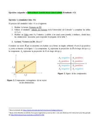
Considere un vector 𝑨
⃗⃗ que se encuentra en el plano 𝑥𝑦 y forma un ángulo arbitrario 𝜃 con el eje positivo
𝑥, como se muestra en la figura 1. La componente 𝐴𝑥 representa la proyección de 𝑨
⃗⃗ a lo largo del eje 𝑥, y
la componente 𝐴𝑦 representa la proyección de 𝐴 a lo largo del eje 𝑦.
Figura 2. Componentes rectangulares de un vector
en dos dimensiones.
1 Recurso tomado de https://phet.colorado.edu/es/simulations/category/physics
2
Bauer, W. & Westfall,D.(2014). Física para ingenierías y ciencias Vol.1. (2a. ed.) McGraw-Hill Interamericana.Recuperado
de http://bibliotecavirtual.unad.edu.co:2053/?il=700
Figura 2. Signos de las componentes.
2. Las componentes rectangulares de 𝑨
⃗⃗ son:
𝐴𝑥 = 𝐴 cos𝜃 (1)
𝐴𝑦 = 𝐴 sin 𝜃 (2)
Estas componentes pueden ser positivas o negativas, dependiendo del cuadrante en que se
ubica el vector, tal como se muestra en la figura 2. Las magnitudes de estas componentes son
las longitudes de los dos lados de un triángulo rectángulo con una hipotenusa de longitud 𝐴.
Debido a esto, la magnitud y la dirección de 𝑨
⃗⃗ se relacionan con sus componentes mediante
las expresiones:
|𝐴| = 𝐴 = √𝐴𝑥
2
+ 𝐴𝑦
2
(3)
𝜃 = tan−1
𝐴𝑦
𝐴𝑥
(4)
Para especificar completamente un vector 𝑨
⃗⃗ se deben dar sus componentes 𝐴𝑥 y 𝐴𝑦 o su
magnitud y dirección 𝐴 y 𝜃.
Los vectores unitarios se usan para especificar una dirección conocida y no tienen otro
significado físico. Son útiles exclusivamente como una convención para describir una
dirección en el espacio. Se usarán los símbolos 𝒊̂ y 𝒋̂ para representar los vectores unitarios
que apuntan en las direcciones 𝑥 y 𝑦 positivas. Por tanto, la notación del vector unitario para
el vector 𝑨
⃗⃗ es:
𝑨
⃗⃗ = 𝐴𝑥𝒊̂ + 𝐴𝑦𝒋̂ (5)
Debido a la conveniencia contable de los vectores unitarios, para sumar dos o más vectores,
se sumar las componentes 𝑥 y 𝑦 por separado. Considerando otro vector 𝑩
⃗⃗ = 𝐵𝑥𝒊̂ + 𝐵𝑦𝒋̂, el
vector resultante 𝑹
⃗⃗ = 𝑨
⃗⃗ + 𝑩
⃗⃗ es:
𝑹
⃗⃗ = (𝐴𝑥 + 𝐵𝑥)𝒊̂ + (𝐴𝑦 + 𝐵𝑦)𝒋̂ (6)
En la figura 3 se muestra la construcción geométrica para la suma de dos vectores mediante
la relación entre las componentes del resultante 𝑹
⃗⃗ y las componentes de los vectores
individuales
3. Figura 3. Construcción geométrica para la suma de dos vectores.
2. Simulador Movimiento de un Proyectil
En la tabla 3 se presentan dos tutoriales, el primero de ellos muestra el paso a paso de cómo
se utiliza el simulador y segundo explica cómo se genera el enlace de la grabación del vídeo.
Descripción Enlace vídeo explicativo Enlace página del recurso
Simulador Adición de Vectores
https://phet.colorado.edu/es/simu
lation/vector-addition
Screencast-o-matic para la grabación y
generación del enlace del vídeo.
https://youtu.be/QgB-Q7Ic-
d0
https://screencast-o-matic.com/
Tabla 3. Vídeo tutoriales que explican el proceso para utilizar el simulador y para generar
el enlace de grabación del vídeo.
Descripción del proceso:
a) Ingresar al simulador: https://phet.colorado.edu/es/simulation/vector-addition
b) Ingresar a la sección Ecuaciones.
c) Verificar que aparezca cuadrícula y el vector 𝒄
⃗ .
d) Variar los Vectores Base en el recuadro
5. 𝑎𝑥 0 -2.0 -102.5 -4.0 -119.7 -6.0 -140.2 -8.0 -159.4 -10 -174.3
𝑎𝑦 0 9.2 -9.0 8.1 -7.0 7.8 -5.0 8.5 -3.0 10 -1.0
𝑎𝑥 5 3.0 -77.9 1.0 -85.2 -1.0 -95.7 -3.0 -110.6 -5.0 -129.8
𝑎𝑦 -5 14.3 -14 12 -12 10 -10 8.5 -8.0 7.8 -6.0
𝑎𝑥 10 8.0 -67.2 6.0 -70.6 4.0 -75.1 2.0 -81.3 0 -90
𝑎𝑦 -10 20.6 -19 18 -17 15.5 -15 13.2 -13 11 -11
Tabla 5. Resultados para 𝑎 − 𝑏
⃗ = 𝑐.
Para 𝑎 + 𝑏
⃗ + 𝑐 = 0
𝒄𝒙 𝜽 𝑏𝑥 𝑏𝑦 𝑏𝑥 𝑏𝑦 𝑏𝑥 𝑏𝑦 𝑏𝑥 𝑏𝑦 𝑏𝑥 𝑏𝑦
|𝒄
⃗ | 𝒄𝒚 2 9 4 7 6 5 8 3 10 1
𝑎𝑥 -10 8 -67,2 6.0 -70.6 4.0 -75.1 2.0 -81.3 0 -90
𝑎𝑦 10 20,6 -19 18 -17 15.5 -15 13.2 -13 11 -11
𝑎𝑥 -5 3.0 -77.9 1.0 -85.2 -1.0 -95.7 -3 -110.6 -5.0 129.8
𝑎𝑦 5 14.3 -14 12 -12 10 -10 8.5 -8 7.8 -6.0
𝑎𝑥 0 -2.0 -102.5 -4.0 -119.7 -6 140.2 -8.0 -159.4 -10 -174.3
𝑎𝑦 0 9.2 -9.0 8.1 -7.0 7.8 -5 8.5 -3.0 10 -1.0
𝑎𝑥 5 -7.0 -150.3 -9.0 -167.5 -11 -180 -13 171.3 -15 165.1
𝑎𝑦 -5 8.1 -4.0 9.2 -2.0 11 0 13.2 2.0 15.5 4.0
𝑎𝑥 10 -12 175.2 -14 167.9 -16 162.6 -18 158.7 -20 155.8
𝑎𝑦 -10 12 1.0 14.3 3.0 16.8 5.0 19.3 7.0 21.9 9.0
Tabla 6. Resultados para 𝑎 + 𝑏
⃗ + 𝑐 = 0.
NOTA: Todo el proceso descrito entre a) y e) no debe quedar grabado en el vídeo.
3. Vídeo
Los requerimientos de la grabación del vídeo son los siguientes:
i. Al inicio, se presenta y se muestra en primer plano ante la cámara del computador.
Debe mostrar su documento de identidad donde se vea claramente sus nombres y
apellidos, ocultando el número del documento por seguridad.
ii. La cámara de su computador debe permanecer como una ventana flotante, de tal
manera que su rostro sea visible durante toda la grabación.
iii. El vídeo debe durar entre 4 y 5 minutos.
iv. En el vídeo graba las simulaciones realizadas para responder únicamente las
preguntas de la tabla 7.
Con base en el trabajo realizado en el simulador y la revisión de la lectura “Vectores en 2D.”
responda y justifique las preguntas asignadas en la tabla 7. Además, copie el enlace de
grabación del vídeo.
Preguntas que debe responder en el vídeo y justificar utilizando el simulador
6. a) Demostrar gráficamente en el simulador que la suma de dos vectores es independiente del orden de la
suma.
b) Demostrar mediante las ecuaciones (3), (4) y (6) alguno de los resultados de la tabla 4.
c) Para uno de los resultados de la tabla 6, demostrar que 𝑎 + 𝑏
⃗ + 𝑐 = 0
d) ¿La magnitud de un vector puede tener un valor negativo? Explique.
e) ¿La ecuación (4) para encontrar la dirección de un vector, sirve para todos los cuadrantes? Verificar
en cada caso.
Respuesta (s):
a)
b)
𝐸𝑐𝑢𝑎𝑐𝑖𝑜𝑛 3
𝑉𝑎𝑙𝑜𝑟𝑒𝑠
𝑎𝑥 = −10 𝑎𝑦 = 10
𝑏𝑥 = 4 𝑏𝑦 = 7
|𝐴| = 𝐴 = √𝐴𝑥
2
+ 𝐴𝑦
2
𝑅𝑒𝑒𝑚𝑝𝑙𝑎𝑧𝑎𝑚𝑜𝑠
|𝐴| = 𝐴 = √(−10)2 + (10)2
𝐴 = √100 + 100
9. c) Para uno de los resultados de la tabla 6, demostrar que 𝑎 + 𝑏
⃗ + 𝑐 = 0
𝑎𝑥 = 5
𝑏𝑥 = 2
𝑐𝑥 = −7
5 + 2 + (−7) = 0
10. d) ¿La magnitud de un vector puede tener un valor negativo? Explique.
No puede tener una magnitud negativa ya que es una distancia y está siempre será positiva
e) ¿La ecuación (4) para encontrar la dirección de un vector, sirve para todos los cuadrantes? Verificar
en cada caso
si ya que un vector unitario se usa para especificar un dirección .
Enlace de grabación del vídeo:
Ejercicio 2. Movimiento Unidimensional (Estudiante # 2)
Desde un observatorio astronómico se reportan las siguientes observaciones
intergalácticas:
Nombre Galaxia Distancia [Mly*] Velocidad [km/s]
G1 2676 18732
G2 1246 8722
G3 7256 7256
G4 11232 78624
G5
242
1694
G6 15435. 108045
Tabla 8. Distancia y velocidad de cada galaxia.
*Mly son las unidades usadas en astronomía conocidas como Años Luz (en
inglés Light Year [Ly]) El prefijo M (Mega) corresponde a la potencia 106
.
** Las comas equivalen a la separación de cifras decimales.
11. A partir de la información del anterior:
a) Realice una gráfica de Velocidad vs Distancia con los datos de la tabla. NOTA:
en el momento en que realice la gráfica en el informe, incluya su nombre en
el título y coloque el origen de coordenadas en el observatorio.
b) ¿qué tipo de gráfica se obtiene? ¿Cuál es la relación entre la velocidad y la
distancia?
c) A partir de la relación encontrada responda:
1. ¿El sistema de galaxias reportado se expande o se contrae? Justifique
su respuesta.
2. Una galaxia G7 viaja a 10,000 [km/s], ¿a qué distancia se encuentra?
3. Una galaxia G8 se encuentra a 18,60 [MLy], ¿a qué velocidad se
mueve?
d) ¿El sistema reportado presenta aceleración? Justifique su respuesta.
a) Realice una gráfica de Velocidad vs Distancia con los datos de la tabla. NOTA:
en el momento en que realice la gráfica en el informe, incluya su nombre en
el título y coloque el origen de coordenadas en el observatorio.
b) ¿qué tipo de gráfica se obtiene? ¿Cuál es la relación entre la velocidad y la
distancia?
12. Se obtiene una gráfica una línea recta ya que la distancia es proporcional a la
velocidad
c)A partir de la relación encontrada responda:
1. ¿El sistema de galaxias reportado se expande o se contrae? Justifique
su respuesta.
El sistema se contrae ya que a mayor velocidad menor distancia
2. Una galaxia G7 viaja a 10,000 [km/s], ¿a qué distancia se encuentra?
𝑉 = 10,000 𝑘𝑚/𝑠
𝑑 = ?
𝑚 = ?
𝑚 =
𝑦2 − 𝑦1
𝑥2 − 𝑥1
𝑚 =
10,8 − 0,122
15,4 − 0,174
= 0,70
D =
V
m
=
10,000 Km/h
0,70
Km/h
MLy
= 14285,71𝑀𝐿𝑦
3. Una galaxia G8 se encuentra a 18,60 [MLy], ¿a qué velocidad se
mueve?
𝐷 = 18,60 𝑀𝐿𝑦
𝑉 =?
M= 0.70
𝑉 = 0,70 ∗ 𝐷
𝑉 = 0,70
𝐾𝑚/ℎ
𝑀𝐿𝑦
∗ 18,60𝑀𝐿𝑦 = 13,02 𝐾𝑚/ℎ
d) ¿El sistema reportado presenta aceleración? Justifique su respuesta.
El sistema no presenta aceleración ya que la velocidad y la distancia son
proporcionales.