Downloaded 33 times
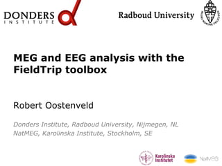

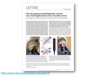
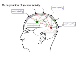
![Some FieldTrip basics
dataout = functionname(cfg, datain, …)
functionname(cfg, datain, …)
dataout = functionname(cfg)
the “cfg” argument is a configuration structure, e.g.
cfg.channel = {‘C3’, C4’, ‘F3’, ‘F4’}
cfg.foilim = [1 70]](https://image.slidesharecdn.com/eegmegandfieldtrip-220908065222-bef3a6da/85/EEG-MEG-and-FieldTrip-61-320.jpg)
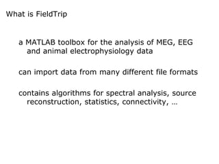
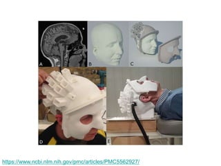
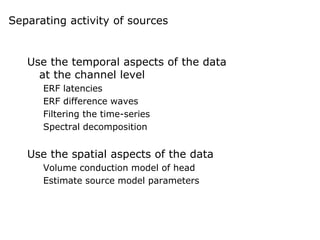
![Using functions in an analysis protocol
ft_preprocessing
ft_rejectartifact
ft_freqanalysis
ft_multiplotTFR ft_freqstatistics
ft_multiplotTFR
FT_PREPROCESSING reads MEG and/or EEG data according to user-specified
trials and applies several user-specified preprocessing steps to the
signals.
Use as
[data] = ft_preprocessing(cfg)
or
[data] = ft_preprocessing(cfg, data)
The first input argument "cfg" is the configuration structure, which
contains all details for the dataset filenames, trials and the
preprocessing options. You can only do preprocessing after defining the
segments of data to be read from the file (i.e. the trials), which is for
example done based on the occurence of a trigger in the data.
...](https://image.slidesharecdn.com/eegmegandfieldtrip-220908065222-bef3a6da/85/EEG-MEG-and-FieldTrip-63-320.jpg)
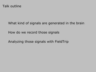
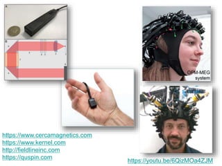
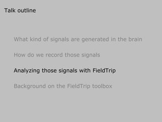
![Using functions in an analysis protocol
ft_preprocessing
ft_rejectartifact
ft_freqanalysis
ft_multiplotTFR ft_freqstatistics
ft_multiplotTFR
cfg = [ ]
cfg.dataset = ‘Subject01.ds’
cfg.bpfilter = [0.01 150]
...
rawdata = ft_preprocessing(cfg)](https://image.slidesharecdn.com/eegmegandfieldtrip-220908065222-bef3a6da/85/EEG-MEG-and-FieldTrip-64-320.jpg)
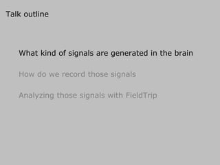
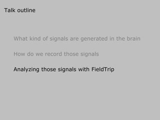
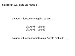
![Using functions in an analysis protocol
ft_preprocessing
ft_rejectartifact
ft_freqanalysis
ft_multiplotTFR ft_freqstatistics
ft_multiplotTFR
cfg = [ ]
cfg.method = ‘mtmfft’
cfg.foilim = [1 120]
...
freqdata = ft_freqanalysis(cfg, rawdata)](https://image.slidesharecdn.com/eegmegandfieldtrip-220908065222-bef3a6da/85/EEG-MEG-and-FieldTrip-65-320.jpg)
![Raw data structure
rawData =
label: {151x1 cell}
trial: {1x80 cell}
time: {1x80 cell}
fsample: 300
hdr: [1x1 struct]
cfg: [1x1 struct]](https://image.slidesharecdn.com/eegmegandfieldtrip-220908065222-bef3a6da/85/EEG-MEG-and-FieldTrip-66-320.jpg)
![Event related response
timelockData =
label: {151x1 cell}
avg: [151x900 double]
var: [151x900 double]
time: [1x900 double]
dimord: 'chan_time’
cfg: [1x1 struct]](https://image.slidesharecdn.com/eegmegandfieldtrip-220908065222-bef3a6da/85/EEG-MEG-and-FieldTrip-67-320.jpg)
![Example use in scripts
cfg = []
cfg.dataset = ‘Subject01.ds’
cfg.bpfilter = [0.01 150]
...
rawdata = ft_preprocessing(cfg)
cfg = []
cfg.method = ‘mtmfft’
cfg.foilim = [1 120]
...
freqdata = ft_freqanalysis(cfg, rawdata)
cfg = []
cfg.method = ‘montecarlo’
cfg.statistic = ‘indepsamplesT’
cfg.design = [1 2 1 2 2 1 2 1 1 2 ... ]
...
freqstat = ft_freqstatistics(cfg, freqdata)
ft_preprocessing
ft_freqanalysis
ft_freqstatistics
ft_topoplotTFR
…](https://image.slidesharecdn.com/eegmegandfieldtrip-220908065222-bef3a6da/85/EEG-MEG-and-FieldTrip-68-320.jpg)
![Example use in scripts
cfg = []
cfg.dataset = ‘Subject01.ds’
cfg.bpfilter = [0.01 150]
...
rawdata = ft_preprocessing(cfg)
cfg = []
cfg.method = ‘mtmfft’
cfg.foilim = [1 120]
...
freqdata = ft_freqanalysis(cfg, rawdata)
cfg = []
cfg.method = ‘montecarlo’
cfg.statistic = ‘indepsamplesT’
cfg.design = [1 2 1 2 2 1 2 1 1 2 ... ]
...
freqstat = ft_freqstatistics(cfg, freqdata)
ft_preprocessing
ft_freqanalysis
ft_freqstatistics
ft_topoplotTFR
…](https://image.slidesharecdn.com/eegmegandfieldtrip-220908065222-bef3a6da/85/EEG-MEG-and-FieldTrip-69-320.jpg)
![Example use in scripts
cfg = []
cfg.dataset = ‘Subject01.ds’
cfg.bpfilter = [0.01 150]
...
rawdata = ft_preprocessing(cfg)
cfg = []
cfg.method = ‘mtmfft’
cfg.foilim = [1 120]
...
freqdata = ft_freqanalysis(cfg, rawdata)
cfg = []
cfg.method = ‘montecarlo’
cfg.statistic = ‘indepsamplesT’
cfg.design = [1 2 1 2 2 1 2 1 1 2 ... ]
...
freqstat = ft_freqstatistics(cfg, freqdata)
ft_preprocessing
ft_freqanalysis
ft_freqstatistics
ft_topoplotTFR
…](https://image.slidesharecdn.com/eegmegandfieldtrip-220908065222-bef3a6da/85/EEG-MEG-and-FieldTrip-70-320.jpg)
![Example use in scripts
cfg = []
cfg.dataset = ‘Subject01.ds’
cfg.bpfilter = [0.01 150]
...
rawdata = ft_preprocessing(cfg)
cfg = []
cfg.method = ‘mtmfft’
cfg.foilim = [1 120]
...
freqdata = ft_freqanalysis(cfg, rawdata)
cfg = []
cfg.method = ‘montecarlo’
cfg.statistic = ‘indepsamplesT’
cfg.design = [1 2 1 2 2 1 2 1 1 2 ... ]
...
freqstat = ft_freqstatistics(cfg, freqdata)
ft_preprocessing
ft_freqanalysis
ft_freqstatistics
ft_topoplotTFR
…](https://image.slidesharecdn.com/eegmegandfieldtrip-220908065222-bef3a6da/85/EEG-MEG-and-FieldTrip-71-320.jpg)
![Example use in scripts
cfg = []
cfg.dataset = ‘Subject01.ds’
cfg.bpfilter = [0.01 150]
...
rawdata = ft_preprocessing(cfg)
cfg = []
cfg.method = ‘mtmfft’
cfg.foilim = [1 120]
...
freqdata = ft_freqanalysis(cfg, rawdata)
cfg = []
cfg.method = ‘montecarlo’
cfg.statistic = ‘indepsamplesT’
cfg.design = [1 2 1 2 2 1 2 1 1 2 ... ]
...
freqstat = ft_freqstatistics(cfg, freqdata)
ft_preprocessing
ft_freqanalysis
ft_freqstatistics
ft_topoplotTFR
…](https://image.slidesharecdn.com/eegmegandfieldtrip-220908065222-bef3a6da/85/EEG-MEG-and-FieldTrip-72-320.jpg)
![Example use in scripts
subj = {‘S01.ds’, ‘S02.ds’, …}
trig = [1 3 7 9]
for s=1:nsubj
for c=1:ncond
cfg = []
cfg.dataset = subj{s}
cfg.trigger = trig(c)
rawdata{s,c} = ft_preprocessing(cfg)
cfg = []
cfg.method = ‘mtmfft’
cfg.foilim = [1 120]
freqdata{s,c} = ft_freqanalysis(cfg, rawdata{s,c})
end
end](https://image.slidesharecdn.com/eegmegandfieldtrip-220908065222-bef3a6da/85/EEG-MEG-and-FieldTrip-73-320.jpg)
![Example use in scripts
subj = {‘S01.ds’, ‘S02.ds’, …}
trig = [1 3 7 9]
for s=1:nsubj
for c=1:ncond
cfg = []
cfg.dataset = subj{s}
cfg.trigger = trig(c)
rawdata = ft_preprocessing(cfg)
filename = sprintf(‘raw%s_%d.mat’, subj{s}, trig(c));
save(filename, ‘rawdata’)
end
end](https://image.slidesharecdn.com/eegmegandfieldtrip-220908065222-bef3a6da/85/EEG-MEG-and-FieldTrip-74-320.jpg)
![Example use in distributed computing
subj = {‘S01.ds’, ‘S02.ds’, …}
trig = [1 3 7 9]
for s=1:nsubj
for c=1:ncond
cfgA{s,c} = []
cfgA{s,c}.dataset = subj{s}
cfgA{s,c}.trigger = trig(c)
cfgA{s,c}.outputfile = sprintf(‘raw%s_%d.mat’, subj{s}, trig(c))
cfgB{s,c} = []
cfgB{s,c}.dataset = subj{s}
cfgB{s,c}.trigger = trig(c)
cfgB{s,c}.inputfile = sprintf(‘raw%s_%d.mat’, subj{s}, trig(c));
cfgB{s,c}.outputfile = sprintf(‘freq%s_%d.mat’, subj{s}, trig(c));
end
end
qsubcellfun(@ft_preprocessing, cfgA)
qsubcellfun(@ft_freqanalysis, cfgB)](https://image.slidesharecdn.com/eegmegandfieldtrip-220908065222-bef3a6da/85/EEG-MEG-and-FieldTrip-75-320.jpg)


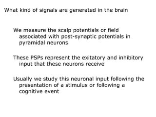
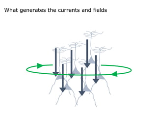
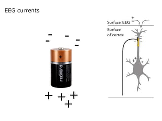
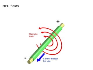
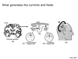
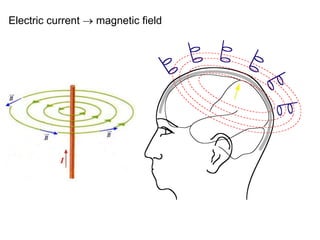
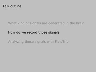
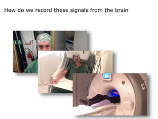
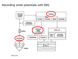
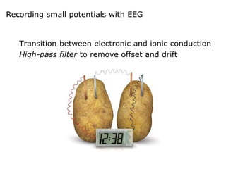
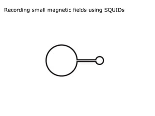
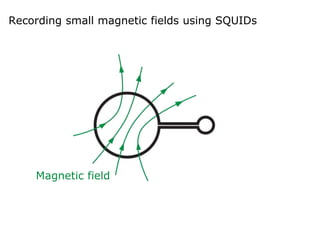
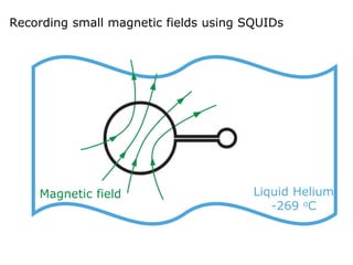
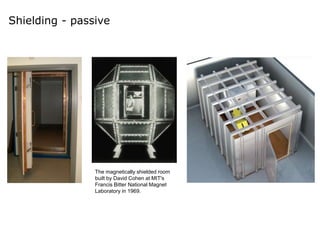
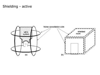
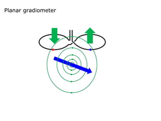
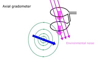
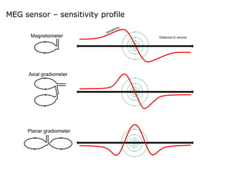
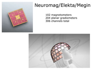
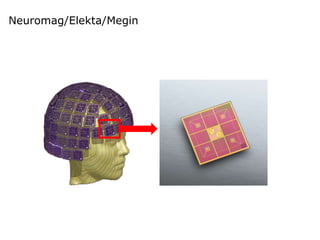
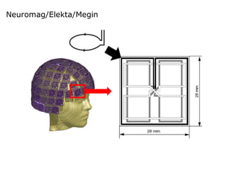
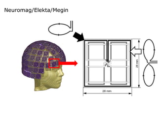
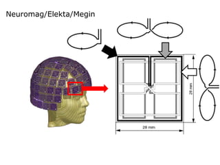
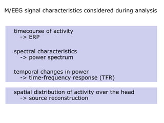
This document summarizes a presentation about analyzing MEG and EEG data with the FieldTrip toolbox. It discusses: 1) What kinds of signals are generated in the brain and how MEG and EEG record those signals. 2) An overview of the analysis process in FieldTrip including preprocessing, time-frequency analysis, and source reconstruction. 3) Examples of how to use different FieldTrip functions together in an analysis pipeline.


