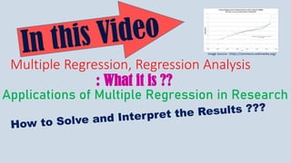
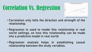
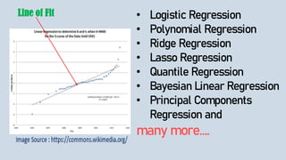
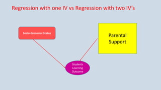
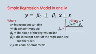
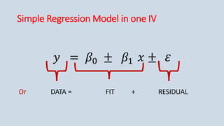
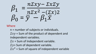
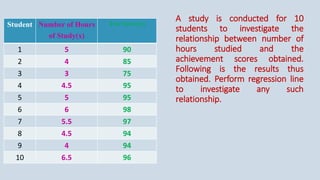
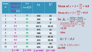
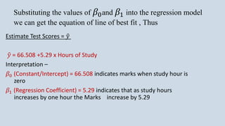
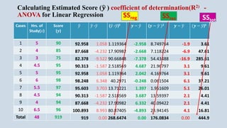
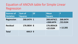
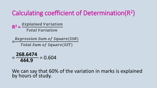
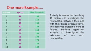
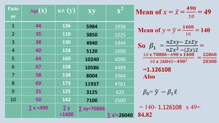
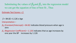
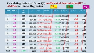
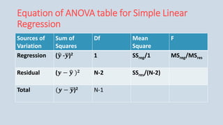
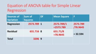
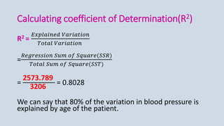
The document provides an overview of multiple regression analysis, explaining its significance in research and differentiating it from correlation. It outlines various types of regression (e.g., linear, logistic, polynomial) and provides examples of regression analysis applied to student study hours and patient age with blood pressure. The document concludes with calculations of regression coefficients and the coefficient of determination, indicating how study hours and age impact their respective outcomes.

1. Image Source : https://commons.wikimedia.org/

2. Multiple Regression, Regression Analysis
: What it is ??
Applications of Multiple Regression in Research

3. Correlation Vs. Regression
• Correlation only tells the direction and strength of the
relationship.
• Regression is used to model this relationship in real
world settings, on how this relationship can be made
into a predictive model in real world.
• Regression analysis helps in establishing causal
relationship between the study variables.

4. Line of Fit • Logistic Regression
• Polynomial Regression
• Ridge Regression
• Lasso Regression
• Quantile Regression
• Bayesian Linear Regression
• Principal Components
Regression and
many more….

5. Students
Learning
Outcome
Socio-Economic Status
Parental
Support
Regression with one IV vs Regression with two IV’s

6. Regression Analysis Basics
•Most used technique in Social and behaviourial sciences.
•It tries to identify and evaluate the relationship between a dependent
variable and one or more independent variables (predictor or
explanatory variable)
•A Model of the relationship is estimated by a regression equation.
•If the model sound enough , may be used to predict the value of
dependent variable.

7. Linear Regression vs. Multiple Regression
•When only one dependent variable and one
independent variable are involved.- Linear
Regression
•When several independent variables are
involved and is used to predict a dependent
variable- Multiple Regression

8. Simple Regression Model in one IV
𝑦 = 𝛽0 ± 𝛽1 𝑥 ± 𝜀
Where Slope
𝑥= independent variable 𝛽1
𝑦= dependent variable 𝛽0
𝛽1 = The slope of the regression line
𝛽0= The intercept point of the regression line
and the y axis
𝜀1= Residual or error terms

9. Simple Regression Model in one IV
𝑦 = 𝛽0 ± 𝛽1 𝑥 ± 𝜀
Or DATA = FIT + RESIDUAL

10. 𝛽1 =
𝑛𝛴𝑥𝑦− 𝛴𝑥𝛴𝑦
𝑛𝛴𝑥2 −(𝛴𝑥)2
𝛽0 = ത
𝑦 − 𝛽1 ҧ
𝑥
Where
n = number of subjects or individuals.
𝛴𝑥𝑦 = Sum of the product of dependent and
independent variables.
𝛴𝑥 = Sum of Independent variable.
𝛴𝑦= Sum of dependent variable.
𝛴𝑥2
= Sum of square of independent variable

11. A study is conducted for 10
students to investigate the
relationship between number of
hours studied and the
achievement scores obtained.
Following is the results thus
obtained. Perform regression line
to investigate any such
relationship.
Student Number of Hours
of Study(x)
Test Score(y)
1 5 90
2 4 85
3 3 75
4 4.5 95
5 5 95
6 6 98
7 5.5 97
8 4.5 94
9 4 94
10 6.5 96

12. = 91.9- 5.29 x 4.8 =
66.508
Stude
nt
Number of
Hours of
Study(x)
Test
Score(y)
xy X2
1 5 90 450 25
2 4 85 340 16
3 3 75 225 9
4 4.5 95 427.5 20.25
5 5 95 475 25
6 6 98 588 36
7 5.5 97 533.5 30.25
8 4.5 94 423 20.25
9 4 94 376 16
10 6.5 96 624 42.25
∑ x =48 ∑ y =919 ∑ xy=4462 ∑X2 = 240
Mean of 𝑥 = ҧ
𝑥 =
48
10
= 4.8
Mean of 𝑦 = ത
𝑦 =
𝟗𝟏𝟗
10
= 91.9
10 𝐱 4462−48 𝐱 919
10 𝐱 240−482 =
508
96
=5.29
So 𝛽1 =
𝑛𝛴𝑥𝑦− 𝛴𝑥𝛴𝑦
𝑛𝛴𝑥2 −(𝛴𝑥)2
=
Also
𝛽0= ത
𝑦 − 𝛽1 ҧ
𝑥

13. Substituting the values of 𝛽0and 𝛽1 into the regression model
we can get the equation of line of best fit , Thus
Estimate Test Scores = ො
𝑦
ො
𝑦 = 66.508 +5.29 x Hours of Study
Interpretation –
𝛽0 (Constant/Intercept) = 66.508 indicates marks when study hour is
zero
𝛽1 (Regression Coefficient) = 5.29 indicates that as study hours
increases by one hour the Marks increase by 5.29

14. Calculating Estimated Score (ෝ
𝒚 ) coefficient of determination(R2) -
ANOVA for Linear Regression
Cases Hrs. of
Study(𝑥)
Score
(𝒚)
ො
𝑦 ො
𝑦 -ത
𝑦 (ො
𝑦 -ത
𝑦)2 𝒚 − ො
𝑦 (𝒚 − ො
𝑦 )𝟐 𝒚 − ത
𝑦 (𝒚 − ത
𝑦)2
1 5 90 92.958 1.058 1.119364 -2.958 8.749764 -1.9 3.61
2 4 85 87.668 -4.232 17.90982 -2.668 7.118224 -6.9 47.61
3 3 75 82.378 -9.522 90.66848 -7.378 54.43488 -16.9 285.61
4 4.5 95 90.313 -1.587 2.518569 4.687 21.96797 3.1 9.61
5 5 95 92.958 1.058 1.119364 2.042 4.169764 3.1 9.61
6 6 98 98.248 6.348 40.2971 -0.248 0.061504 6.1 37.21
7 5.5 97 95.603 3.703 13.71221 1.397 1.951609 5.1 26.01
8 4.5 94 90.313 -1.587 2.518569 3.687 13.59397 2.1 4.41
9 4 94 87.668 -4.232 17.90982 6.332 40.09422 2.1 4.41
10 6.5 96 100.893 8.993 80.87405 -4.893 23.94145 4.1 16.81
Total 48 919 919 0.00 268.6474 0.00 176.0834 0.00 444.9
SSreg SSres SStot

15. Equation of ANOVA table for Simple Linear
Regression
Sources of
Variation
Sum of
Squares
Df Mean
Square
F
Regression (ෝ
𝒚 -ഥ
𝒚)2 1 SSreg/1 MSreg/MSres
Residual (𝒚 − ෝ
𝒚 )𝟐 N-2 SSres/(N-2)
Total (𝒚 − ഥ
𝒚)2 N-1

16. Equation of ANOVA table for Simple Linear
Regression
Sources of
Variation
Sum of
Squares
Df Mean
Square
F
Regression 268.6474 1 268.6474/1
=268.6474
268.6474
/22.0104
= 12.205
Residual 176.0834 8 176.0834/8
=22.0104
Total 444.9 9

17. Calculating coefficient of Determination(R2)
R2 =
𝐸𝑥𝑝𝑙𝑎𝑖𝑛𝑒𝑑 𝑉𝑎𝑟𝑖𝑎𝑡𝑖𝑜𝑛
𝑇𝑜𝑡𝑎𝑙 𝑉𝑎𝑟𝑖𝑎𝑡𝑖𝑜𝑛
=
𝑅𝑒𝑔𝑟𝑒𝑠𝑠𝑖𝑜𝑛 𝑆𝑢𝑚 𝑜𝑓 𝑆𝑞𝑢𝑎𝑟𝑒(𝑆𝑆𝑅)
𝑇𝑜𝑡𝑎𝑙 𝑆𝑢𝑚 𝑜𝑓 𝑆𝑞𝑢𝑎𝑟𝑒(𝑆𝑆𝑇)
=
268.6474
444.9
= 0.604
We can say that 60% of the variation in marks is explained
by hours of study.

18. One more Example…..
A study is conducted involving
10 patients to investigate the
relationship between their age
with their blood pressure level.
The observed outcome were as
follows. Perform regression
analysis to investigate the
existence of any such
relationship.
Patient Age (x) Blood Pressure (y)
1 44 136
2 35 110
3 38 130
4 40 128
5 64 160
6 67 158
7 58 138
8 69 173
9 25 125
10 50 142

19. = 140- 1.126108 x 49=
84.82
Patie
nt
Age(x) B.P. (y) xy x2
1 44 136 5984 1936
2 35 110 3850 1225
3 38 130 4940 1444
4 40 128 5120 1600
5 64 160 10240 4096
6 67 158 10586 4489
7 58 138 8004 3364
8 69 173 11937 4761
9 25 125 3125 625
10 50 142 7100 2500
∑ x =490 ∑ y
=1400
∑ xy=70886
∑ x2=26040
Mean of 𝑥 = ҧ
𝑥 =
𝟒𝟗𝟎
10
= 49
Mean of 𝑦 = ത
𝑦 =
𝟏𝟒𝟎𝟎
10
= 140
10 𝐱 𝟕𝟎𝟖𝟖𝟔−4𝟗𝟎 𝐱 𝟏𝟒𝟎𝟎
10 𝐱 2𝟔𝟎40−𝟒𝟗𝟎2 =
𝟐𝟐𝟖𝟔𝟎
𝟐𝟎𝟑𝟎𝟎
=1.126108
So 𝛽1 =
𝑛𝛴𝑥𝑦− 𝛴𝑥𝛴𝑦
𝑛𝛴𝑥2 −(𝛴𝑥)2
=
Also
𝛽0= ത
𝑦 − 𝛽1 ҧ
𝑥

20. Substituting the values of 𝛽0and 𝛽1 into the regression model
we can get the equation of line of best fit , Thus
Estimate Test Scores = ො
𝑦
ො
𝑦 = 84.82 +1.126 x Age
Interpretation –
𝛽0 (Constant/Intercept) = 84.82 indicates blood pressure when age is
zero
𝛽1 (Regression Coefficient) = 1.126 indicates that as age increases by
one year the BP increases by 1.126

21. Calculating Estimated Score (ෝ
𝒚 ) coefficient of determination(R2) -
ANOVA for Linear Regression
Cases Age(𝑥) BP
(𝒚)
ො
𝑦 ො
𝑦 -ത
𝑦 (ො
𝑦 -ത
𝑦)2 𝒚 − ො
𝑦 (𝒚 − ො
𝑦 )𝟐 𝒚 − ത
𝑦 (𝒚 − ത
𝑦)2
1 44 136 134.364 -5.636 31.7645 1.6362.676496 -4 16
2 35 110 124.23 -15.77 248.6929 -14.23202.4929 -30 900
3 38 130 127.608 -12.392 153.5617 2.3925.721664 -10 100
4 40 128 129.86 -10.14 102.8196 -1.86 3.4596 -12 144
5 64 160 156.884 16.884 285.0695 3.1169.709456 20 400
6 67 158 160.262 20.262 410.5486 -2.2625.116644 18 324
7 58 138 150.128 10.128 102.5764 -12.128147.0884 -2 4
8 69 173 162.514 22.514 506.8802 10.486109.9562 33 1089
9 25 125 112.97 -27.03 730.6209 12.03144.7209 -15 225
10 50 142 141.12 1.12 1.2544 0.88 0.7744 2 4
Total 490 1400 1400 0.00 2573.789 0.00 631.716 0.00 3206
SSreg SSres SStot

22. Equation of ANOVA table for Simple Linear
Regression
Sources of
Variation
Sum of
Squares
Df Mean
Square
F
Regression (ෝ
𝒚 -ഥ
𝒚)2 1 SSreg/1 MSreg/MSres
Residual (𝒚 − ෝ
𝒚 )𝟐 N-2 SSres/(N-2)
Total (𝒚 − ഥ
𝒚)2 N-1

23. Equation of ANOVA table for Simple Linear
Regression
Sources of
Variation
Sum of
Squares
Df Mean Square F
Regression 2573.789 1 2573.789/1
=2573.789
2573.789
/78.9645
= 32.594
Residual 631.716 8 631.71/8
=78.9645
Total 3206 9

24. Calculating coefficient of Determination(R2)
R2 =
𝐸𝑥𝑝𝑙𝑎𝑖𝑛𝑒𝑑 𝑉𝑎𝑟𝑖𝑎𝑡𝑖𝑜𝑛
𝑇𝑜𝑡𝑎𝑙 𝑉𝑎𝑟𝑖𝑎𝑡𝑖𝑜𝑛
=
𝑅𝑒𝑔𝑟𝑒𝑠𝑠𝑖𝑜𝑛 𝑆𝑢𝑚 𝑜𝑓 𝑆𝑞𝑢𝑎𝑟𝑒(𝑆𝑆𝑅)
𝑇𝑜𝑡𝑎𝑙 𝑆𝑢𝑚 𝑜𝑓 𝑆𝑞𝑢𝑎𝑟𝑒(𝑆𝑆𝑇)
=
2573.789
3206
= 0.8028
We can say that 80% of the variation in blood pressure is
explained by age of the patient.

25. Thanks
E-mail:
drvsinghonline@gmail.co
m
Mob: +91-9438574139
© V. Singh
© V. Singh