The document describes how to manipulate the brightness and contrast of an image in MATLAB. It includes steps to: 1. Read in an image, convert it to grayscale, and display the original and grayscale images. 2. Manually adjust the brightness in different regions of the image by multiplying the pixel values by constants. 3. Use MATLAB functions like imadjust and histeq to automatically adjust brightness, contrast, and equalize the image histogram. 4. Explain morphological operations like dilation and erosion that can be used to enhance grayscale images.

1. % Experiencia de Aprendizaje anterior
% Tarea: Manipular el brillo de una imagen
Ic=imread('flores.bmp');
[x,y,z]=size(Ic);
x1=x/2;
y1=y/2;
figure, imshow(Ic), title('Imagen original');
Ig=rgb2gray(Ic);
figure, imshow(Ig), title('Imagen escala de grises');
% + Brillo
for m=1:y1
for n=1:x1
Ig(n,m)=Ig(n,m)*1.3;
end
end
for m=y1+1:y
for n=1:x1
Ig(n,m)=Ig(n,m)*1.6;
end
end
% + Oscuro
for m=1:y1
for n=x1+1:x
Ig(n,m)=Ig(n,m)*0.4;
end
end
for m=y1+1:y
for n=x1+1:x
Ig(n,m)=Ig(n,m)*0.7;
end
end
figure, imshow(Ig);
% NOTA:
% Implementar con programas y/o funciones propias del alumno.
% No usar funciones del matlab para procesamiento imagenes.
% En Practicas Calificadas y Examen final no se consideraràn las funciones
% del Matlab para procesamiento de imagenes.
%Funciones del Matlab "solo para referencia"
% Brillo
Ic=imread('flores.bmp');
figure, imshow(Ic), title('Imagen original');
Ig=rgb2gray(Ic);
figure, imshow(Ig), title('Imagen escala de grises');
% Funcion de matlab para mainuplar brillo y contraste: imadjust
help imadjust
% IMADJUST Adjust image intensity values or colormap.
% J = IMADJUST(I) maps the values in intensity image I to new values in J
% such that 1% of data is saturated at low and high intensities of I.
% This increases the contrast of the output image J.
%
% J = IMADJUST(I,[LOW_IN; HIGH_IN],[LOW_OUT; HIGH_OUT]) maps the values
% in intensity image I to new values in J such that values between LOW_IN
% and HIGH_IN map to values between LOW_OUT and HIGH_OUT. Values below
% LOW_IN and above HIGH_IN are clipped; that is, values below LOW_IN map
% to LOW_OUT, and those above HIGH_IN map to HIGH_OUT. You can use an
% empty matrix ([]) for [LOW_IN; HIGH_IN] or for [LOW_OUT; HIGH_OUT] to
% specify the default of [0 1]. If you omit the argument, [LOW_OUT;

2. % HIGH_OUT] defaults to [0 1].
%
% J = IMADJUST(I,[LOW_IN; HIGH_IN],[LOW_OUT; HIGH_OUT],GAMMA) maps the
% values of I to new values in J as described in the previous syntax.
% GAMMA specifies the shape of the curve describing the relationship
% between the values in I and J. If GAMMA is less than 1, the mapping is
% weighted toward higher (brighter) output values. If GAMMA is greater
% than 1, the mapping is weighted toward lower (darker) output values. If
% you omit the argument, GAMMA defaults to 1 (linear mapping).
J1 = imadjust(Ig);
figure, imshow(J1), title('Ajuste 1');
J1b = imadjust(J1);
figure, imshow(J1b), title('Ajuste 1b');
J2 = imadjust(Ig,[0.3 0.7],[]);
figure, imshow(J2), title('Ajuste 2');
%Usando el Gamma
J3z=imadjust(Ig,[0 1],[0.2 1],0.2);
figure, imshow(J3z), title('Ajuste 3z');
J3=imadjust(Ig,[0 1],[0.2 1],1);
figure, imshow(J3), title('Ajuste 3');
J3b=imadjust(Ig,[0 1],[0.2 1],2);
figure, imshow(J3b), title('Ajuste 3b');
J3c=imadjust(Ig,[0 1],[0.2 1],3);
figure, imshow(J3c), title('Ajuste 3c');
J4 = imadjust(Ig,[0.3 1],[0 1],1);
figure, imshow(J4), title('Ajuste 4');
%Histograma
Ic = imread('flores.bmp');
figure, imshow(Ic), title('Imagen original');
Ig=rgb2gray(Ic);
figure, imshow(Ig), title('Imagen escala de grises');
% Funcion para mostrar el histograma: imhist
help imhist
% IMHIST Display histogram of image data.
% IMHIST(I) displays a histogram for the intensity image I whose number of
% bins are specified by the image type. If I is a grayscale image, IMHIST
% uses 256 bins as a default value. If I is a binary image, IMHIST uses
% only 2 bins.
%
% IMHIST(I,N) displays a histogram with N bins for the intensity image I
% above a grayscale colorbar of length N. If I is a binary image then N
% can only be 2.
%
% IMHIST(X,MAP) displays a histogram for the indexed image X. This
% histogram shows the distribution of pixel values above a colorbar of the
% colormap MAP. The colormap must be at least as long as the largest index
% in X. The histogram has one bin for each entry in the colormap.
%
% [COUNTS,X] = imhist(...) returns the histogram counts in COUNTS and the
% bin locations in X so that stem(X,COUNTS) shows the histogram. For
% indexed images, it returns the histogram counts for each colormap entry;
% the length of COUNTS is the same as the length of the colormap.

3. figure, imhist(Ig);
[c,x]=imhist(Ig);
figure, stem(x,c);
% Ecualizacion del histograma
help histeq
% HISTEQ Enhance contrast using histogram equalization.
% HISTEQ enhances the contrast of images by transforming the values in an
% intensity image, or the values in the colormap of an indexed image, so
% that the histogram of the output image approximately matches a specified
% histogram.
%
% J = HISTEQ(I,HGRAM) transforms the intensity image I so that the histogram
% of the output image J with length(HGRAM) bins approximately matches HGRAM.
% The vector HGRAM should contain integer counts for equally spaced bins
% with intensity values in the appropriate range: [0,1] for images of class
% double or single, [0,255] for images of class uint8, [0,65535] for images
% of class uint16, and [-32768, 32767] for images of class int16. HISTEQ
% automatically scales HGRAM so that sum(HGRAM) = NUMEL(I). The histogram of
% J will better match HGRAM when length(HGRAM) is much smaller than the
% number of discrete levels in I.
%
% J = HISTEQ(I,N) transforms the intensity image I, returning in J an
% intensity image with N discrete levels. A roughly equal number of pixels
% is mapped to each of the N levels in J, so that the histogram of J is
% approximately flat. (The histogram of J is flatter when N is much smaller
% than the number of discrete levels in I.) The default value for N is 64.
%
% [J,T] = HISTEQ(I) returns the gray scale transformation that maps gray
% levels in the intensity image I to gray levels in J.
he = histeq(Ig);
figure, imshow(Ig);
figure, imhist(Ig);
figure, imshow(he);
figure, imhist(he);
hea = histeq(Ig,5);
figure, imshow(hea);
figure, imhist(hea);
hea2 = histeq(Ig,10);
figure, imshow(hea2);
figure, imhist(hea2);
[he,t] = histeq(Ig);
figure, stem(t);
% Operaciones morfologicas I: Dilatacion y erosion de imaganes escala de grises
% OM = EE + I, EE = Elemento estructural
% Dilatación de escala de grises
% Dilatación de imagenes escala de grises
% I imagen
I=[ 0 0 0 0 0 0 0 0 0 0 0;...
0 0 0 0 0 0 0 0 0 0 0;...
0 0 15 15 27 27 8 8 0 0 0;...
0 0 100 100 95 95 1 1 0 0 0;...
0 0 0 0 0 0 0 0 0 0 0;...
0 0 0 0 0 0 0 0 0 0 0;...
64 64 128 128 255 255 255 128 128 64 64;...

4. 64 64 128 128 255 255 255 128 128 64 64;...
0 0 0 0 0 255 255 255 0 0 0;...
0 0 0 0 0 255 255 255 0 0 0;...
0 0 0 0 0 128 128 128 0 0 0;...
0 0 0 0 0 128 128 128 0 0 0;...
0 0 0 0 0 64 64 64 0 0 0;...
0 0 0 0 0 64 64 64 0 0 0;...
0 0 0 0 0 0 0 0 0 0 0;...
0 0 0 0 0 0 0 0 0 0 0]
figure, imshow(imresize(uint8(I),[480,480])), title('imagen original');
% Definicion del elemento estructural
% Funcion para definir el ee: strel
help strel
% STREL Create morphological structuring element.
% SE = STREL('arbitrary',NHOOD) creates a flat structuring element with
% the specified neigbhorhood. NHOOD is a matrix containing 1's and 0's;
% the location of the 1's defines the neighborhood for the morphological
% operation. The center (or origin) of NHOOD is its center element,
% given by FLOOR((SIZE(NHOOD) + 1)/2). You can also omit the 'arbitrary'
% string and just use STREL(NHOOD).
%
% SE = STREL('arbitrary',NHOOD,HEIGHT) creates a nonflat structuring
% element with the specified neighborhood. HEIGHT is a matrix the same
% size as NHOOD containing the height values associated with each nonzero
% element of NHOOD. HEIGHT must be real and finite-valued. You can also
% omit the 'arbitrary' string and just use STREL(NHOOD,HEIGHT).
%
% SE = STREL('ball',R,H,N) creates a nonflat "ball-shaped" (actually an
% ellipsoid) structuring element whose radius in the X-Y plane is R and
% whose height is H. R must be a nonnegative integer, and H must be a
% real scalar. N must be an even nonnegative integer. When N is greater
% than 0, the ball-shaped structuring element is approximated by a
% sequence of N nonflat line-shaped structuring elements. When N is 0, no
% approximation is used, and the structuring element members comprise all
% pixels whose centers are no greater than R away from the origin, and the
% corresponding height values are determined from the formula of the
% ellipsoid specified by R and H. If N is not specified, the default
% value is 8. Note: Morphological operations using ball approximations
% (N>0) run much faster than when N=0.
%
% SE = STREL('diamond',R) creates a flat diamond-shaped structuring
% element with the specified size, R. R is the distance from the
% structuring element origin to the points of the diamond. R must be a
% nonnegative integer scalar.
%
% SE = STREL('disk',R,N) creates a flat disk-shaped structuring element
% with the specified radius, R. R must be a nonnegative integer. N must
% be 0, 4, 6, or 8. When N is greater than 0, the disk-shaped structuring
% element is approximated by a sequence of N (or sometimes N+2)
% periodic-line structuring elements. When N is 0, no approximation is
% used, and the structuring element members comprise all pixels whose
% centers are no greater than R away from the origin. N can be omitted,
% in which case its default value is 4. Note: Morphological operations
% using disk approximations (N>0) run much faster than when N=0. Also,
% the structuring elements resulting from choosing N>0 are suitable for
% computing granulometries, which is not the case for N=0. Sometimes it
% is necessary for STREL to use two extra line structuring elements in the
% approximation, in which case the number of decomposed structuring
% elements used is N+2.
%
% SE = STREL('line',LEN,DEG) creates a flat linear structuring element
% with length LEN. DEG specifies the angle (in degrees) of the line as
% measured in a counterclockwise direction from the horizontal axis.
% LEN is approximately the distance between the centers of the

5. % structuring element members at opposite ends of the line.
%
% SE = STREL('octagon',R) creates a flat octagonal structuring element
% with the specified size, R. R is the distance from the structuring
% element origin to the sides of the octagon, as measured along the
% horizontal and vertical axes. R must be a nonnegative multiple of 3.
%
% SE = STREL('pair',OFFSET) creates a flat structuring element containing
% two members. One member is located at the origin; the second member's
% location is specified by the vector OFFSET. OFFSET must be a
% two-element vector of integers.
%
% SE = STREL('periodicline',P,V) creates a flat structuring element
% containing 2*P+1 members. V is a two-element vector containing
% integer-valued row and column offsets. One structuring element member
% is located at the origin. The other members are located at 1*V, -1*V,
% 2*V, -2*V, ..., P*V, -P*V.
%
% SE = STREL('rectangle',MN) creates a flat rectangle-shaped structuring
% element with the specified size. MN must be a two-element vector of
% nonnegative integers. The first element of MN is the number rows in the
% structuring element neighborhood; the second element is the number of
% columns.
%
% SE = STREL('square',W) creates a square structuring element whose
% width is W pixels. W must be a nonnegative integer scalar.
%
% Notes
% -----
% For all shapes except 'arbitrary', structuring elements are constructed
% using a family of techniques known collectively as "structuring element
% decomposition." The principle is that dilation by some large
% structuring elements can be computed faster by dilation with a sequence
% of smaller structuring elements. For example, dilation by an 11-by-11
% square structuring element can be accomplished by dilating first with a
% 1-by-11 structuring element and then with an 11-by-1 structuring
% element. This results in a theoretical performance improvement of a
% factor of 5.5, although in practice the actual performance improvement
% is somewhat less. Structuring element decompositions used for the
% 'disk' and 'ball' shapes are approximations; all other decompositions
% are exact.
% EE=cuadrado de lado 3 pixeles
ee=strel('square', 3)
ee1 = strel('square',11) % 11-by-11 square
ee2 = strel('line',10,45) % line, length 10, angle 45 degrees
ee3 = strel('disk',10) % disk, radius 10
ee4 = strel('ball',15,5) % ball, radius 15, height 5
% DILATACION
% Funcion Matlab para la dilatacion de imagenes: imdilate
help imdilate
% IMDILATE Dilate image.
% IM2 = IMDILATE(IM,SE) dilates the grayscale, binary, or packed binary
% image IM, returning the dilated image, IM2. SE is a structuring element
% object, or array of structuring element objects, returned by the STREL
% function.
%
% If IM is logical (binary), then the structuring element must be flat
% and IMDILATE performs binary dilation. Otherwise, it performs
% grayscale dilation. If SE is an array of structuring element
% objects, IMDILATE performs multiple dilations, using each
% structuring element in SE in succession.

6. %
% IM2 = IMDILATE(IM,NHOOD) dilates the image IM, where NHOOD is a
% matrix of 0s and 1s that specifies the structuring element
% neighborhood. This is equivalent to the syntax IIMDILATE(IM,
% STREL(NHOOD)). IMDILATE determines the center element of the
% neighborhood by FLOOR((SIZE(NHOOD) + 1)/2).
I1=imdilate(I,ee)
figure, imshow(imresize(uint8(I1),[480,480]));
I3=imread('igsg.bmp');
figure, imshow(I3), title('imagen original');
% Definicion del elemento estructural
ee=strel('square', 30);
% Se aplica dilatacion
I4=imdilate(I3,ee);
figure, imshow(I4), title('imagen dilatada');
% Erosión de imagenes escala de grises
% I imagen
% I imagen
I=[ 0 0 0 0 0 0 0 0 0 0 0;...
0 0 0 0 0 0 0 0 0 0 0;...
0 0 15 15 27 27 8 8 0 0 0;...
0 0 100 100 95 95 1 1 0 0 0;...
0 0 0 0 0 0 0 0 0 0 0;...
0 0 0 0 0 0 0 0 0 0 0;...
64 64 128 128 255 255 255 128 128 64 64;...
64 64 128 128 255 255 255 128 128 64 64;...
0 0 0 0 0 255 255 255 0 0 0;...
0 0 0 0 0 255 255 255 0 0 0;...
0 0 0 0 0 128 128 128 0 0 0;...
0 0 0 0 0 128 128 128 0 0 0;...
0 0 0 0 0 64 64 64 0 0 0;...
0 0 0 0 0 64 64 64 0 0 0;...
0 0 0 0 0 0 0 0 0 0 0;...
0 0 0 0 0 0 0 0 0 0 0]
figure, imshow(imresize(uint8(I),[480,480])), title('imagen original');
% Definicion del elemento estructural
ee=strel('square', 2);
% EROSION
% Funcion Matlab para erosionar una imagen: imerode
help imerode
% IMERODE Erode image.
% IM2 = IMERODE(IM,SE) erodes the grayscale, binary, or packed binary image
% IM, returning the eroded image, IM2. SE is a structuring element
% object, or array of structuring element objects, returned by the
% STREL function.
%
% If IM is logical and the structuring element is flat, IMERODE
% performs binary erosion; otherwise it performs grayscale erosion. If
% SE is an array of structuring element objects, IMERODE performs
% multiple erosions of the input image, using each structuring element
% in succession.
%
% IM2 = IMERODE(IM,NHOOD) erodes the image IM, where NHOOD is an array
% of 0s and 1s that specifies the structuring element. This is
% equivalent to the syntax IMERODE(IM,STREL(NHOOD)). IMERODE uses this
% calculation to determine the center element, or origin, of the

7. % neighborhood: FLOOR((SIZE(NHOOD) + 1)/2).
% Se aplica erosión
I1=imerode(I,ee);
figure, imshow(imresize(uint8(I1),[480,480])), title('Imagen erosionada');
I3=imread('igsg.bmp');
figure, imshow(I3);
% Definicion del elemento estructural
ee=strel('square', 30);
% Se aplica erosión
I4=imerode(I3,ee);
figure, imshow(I4), title('Imagen erosionada');
%=========================================================================
% Operaciones morfologicas II: Dilatacion y erosion de imagenes binarias
% Dilatacion de imagenes binarias:
% TAREA:
% 1. Implementar la dilatacion y erosion en "negro" de imagenes binarias
% 2. Explicar el algoritmo de las funciones dilatacion y erosion implementadas
% 3. Realizar el diagrama de flujo de las funciones implementadas
% Creando una imagen binaria
b=ones(64);
n=zeros(64);
I=[b n b n b n b n; n b n b n b n b];
%I=imread('patron.bmp');
figure, imshow(I), title('Imagen original');
m=strel('square',20);
I1=imdilate(I,m);
figure, imshow(I1), title('Imagen dilatada');
% Erosión de imagenes binarias:
% I=imread('patron.bmp');
I2=[b n b n b n b n; n b n b n b n b];
figure, imshow(I2), title('Imagen original');
m=strel('square',20);
I2=imerode(I2,m);
figure, imshow(I2), title('Imagen erosionada');
% TAREA.
% 1. Explicar el algoritmo de las funciones dilatacion y erosion de la EA
% 2. Realizar el diagrama de flujo de las funciones
% Ejemplos: Con funciones
I=imread('joyas.bmp');
figure, imshow(I), title('Imagen original');
J=rgb2gray(I);
figure, imshow(J), title('Imagen escala de grises');
imwrite(J,'joyasG.bmp');
% K=im2bw(J,0.2);
% K=im2bw(J,0.5);
K=im2bw(J,0.7);
figure, imshow(K), title('Imagen binaria');
imwrite(K,'joyasB.bmp');
% Dilatacion escala de grises
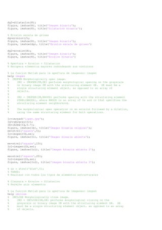
dg=dilatacion(J);
figure, imshow(K), title('Imagen binaria');
figure, imshow(dg), title('Dilatacion escala de grises');

8. dg2=dilatacion(K);
figure, imshow(K), title('Imagen binaria');
figure, imshow(K), title('Dilatacion binaria');
% Erosion escala de grises
dg=erosion(J);
figure, imshow(K), title('Imagen binaria');
figure, imshow(dg), title('Erosion escala de grises')
dg2=erosion(K);
figure, imshow(K), title('Imagen binaria');
figure, imshow(K), title('Erosion binaria')
% Apertura = Erosion + Dilatacion
% Recupera elementos mayores redondeando sus contornos
% La funcion Matlab para la apertura de imagenes: imopen
help imopen
% IMOPEN Morphologically open image.
% IM2 = IMOPEN(IM,SE) performs morphological opening on the grayscale
% or binary image IM with the structuring element SE. SE must be a
% single structuring element object, as opposed to an array of
% objects.
%
% IM2 = IMOPEN(IM,NHOOD) performs opening with the structuring element
% STREL(NHOOD), where NHOOD is an array of 0s and 1s that specifies the
% structuring element neighborhood.
%
% The morphological open operation is an erosion followed by a dilation,
% using the same structuring element for both operations.
Ic=imread('iopen.jpg');
Ig=rgb2gray(Ic);
Ib=im2bw(Ig,0.7);
figure, imshow(Ib), title('Imagen binaria original');
ee=strel('square',5);
Io=imopen(Ib,ee);
figure, imshow(Io), title('Imagen binaria abierta');
ee=strel('square',10);
Io1=imopen(Ib,ee);
figure, imshow(Io1), title('Imagen binaria abierta 2');
ee=strel('square',20);
Io2=imopen(Ib,ee);
figure, imshow(Io2), title('Imagen binaria abierta 3');
% se = strel('disk',5);
% TAREA:
% Realizar con todos los tipos de elementos estructurales
% Clausura = Erosion + Dilatacion
% Permite unir elementos
% La funcion Matlab para la apertura de imagenes: imopen
help imclose
% IMCLOSE Morphologically close image.
% IM2 = IMCLOSE(IM,SE) performs morphological closing on the
% grayscale or binary image IM with the structuring element SE. SE
% must be a single structuring element object, as opposed to an array
% of objects.

9. %
% IMCLOSE(IM,NHOOD) performs closing with the structuring element
% STREL(NHOOD), where NHOOD is an array of 0s and 1s that specifies the
% structuring element neighborhood.
%
% The morphological close operation is a dilation followed by an erosion,
% using the same structuring element for both operations.
figure, imshow(Ib), title('Imagen binaria original');
ee=strel('square',5);
Io=imclose(Ib,ee);
figure, imshow(Io), title('Imagen binaria cerrada');
ee=strel('square',30);
Io1=imclose(Ib,ee);
figure, imshow(Io1), title('Imagen binaria cerrada 2');
ee=strel('square',50);
Io2=imclose(Ib,ee);
figure, imshow(Io2), title('Imagen binaria cerrada 3');
% Extracción de Bordes
% B = I- erosion(I)
% Rellenado de regiones
% 1. Extraer borde
% 2. Se toma un punto (0) dentro del borde
% 3. Erosionar el punto 0. i=1
% 4. Resultado punto nuevo. i=i+1
% 5. Erosionar punto nuevo
% 6. i=npii? No: Paso 4
% 7. Si: Sumar 1. + 5.
%