dsp
•
0 likes•69 views

This document discusses sampling and analog-to-digital conversion. It begins by introducing sampling and the sampling theorem, which states that a continuous-time signal can be uniquely represented by its samples if the sampling frequency is greater than twice the highest frequency present in the signal. It then describes the components and process of analog-to-digital conversion, including periodic sampling, quantization, encoding, and the effects of aliasing if the sampling rate is too low. It also discusses digital-to-analog conversion and reconstruction of the original analog signal from its samples.

Recommended
More Related Content
What's hot
What's hot (20)
Similar to dsp
Similar to dsp (20)
Recently uploaded
Recently uploaded (20)
dsp
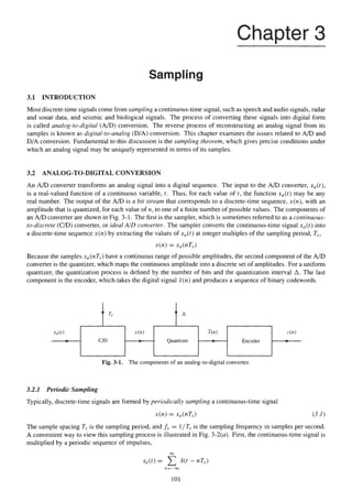
- 1. Chapter 3 Sampling 3.1 INTRODUCTION Most discrete-timesignalscome fromsampling a continuous-timesignal, such as speech and audio signals, radar and sonar data, and seismic and biological signals. The process of converting these signals into digital form is called analog-to-digital (AID)conversion. The reverse process of reconstructing an analog signal from its samples is known as digital-to-analog (D/A)conversion. This chapter examines the issues related to A/D and D/A conversion. Fundamental to this discussion is the sampling theorem, which gives precise conditions under which an analog signal may be uniquely represented in terms of its samples. 3.2 ANALOG-TO-DIGITALCONVERSION An A/D converter transforms an analog signal into a digital sequence. The input to the A/D converter, x,(t), is a real-valued function of a continuous variable, t . Thus, for each value oft, the function x,(t) may be any real number. The output of the A/D is a bit stream that corresponds to a discrete-time sequence, x(n), with an amplitude that is quantized, for each value of n, to one of a finite number of possible values. The components of an A/D converterare shown in Fig. 3- 1. The first is the sampler,which is sometimesreferred to as a continuous- to-discrete ( C P )converter, or ideal AlD converter. The sampler converts the continuous-time signal x,(t) into a discrete-time sequencex(n)by extracting the values of .u,(r) at integer multiples of the sampling period, T,, Because the samplesx,(nTs) have a continuous range of possible amplitudes, the second component of the A/D converteris the quantizer, which maps the continuous amplitude into a discrete set of amplitudes. For a uniform quantizer, the quantization process is defined by the number of bits and the quantization interval A. The last component is the encoder, which takes the digital signal i ( n )and produces a sequence of binary codewords. 3.2.1 Periodic Sampling " Typically, discrete-time signals are formed by periodically sampling a continuous-time signal The sample spacing T, is the samplingperiod, and f, = I/ T, is the sampling frequency in samplesper second. A convenientway to view this sampling process is illustrated in Fig. 3-2(a).First, the continuous-time signal is multiplied by a periodic sequence of impulses, Ts " A *d[) - Fig. 3-1. The components of an analog-to-digital converter. C/D Quantizer *(I?) P 3 ~ ) L , - P Encoder c(n) -
- 2. 102 SAMPLING [CHAP. 3 to form the sampled signal Then, the sampled signal is convertedinto a discrete-timesignalby mapping the impulsesthat are spaced in time by Ts into a sequence x(n)where the sample values are indexed by the integer variable n: This process is illustrated in Fig. 3-2(b). -2Ts -Ts 0 Ts 2Ts 3T, 4T, - 2 - 1 0 1 2 3 4 (b) Fig. 3-2. Continuous-todiscreteconversion. (a)A model that consists of multiplying x,(I) by a sequence of impulses. followed by a system that converts impulses into samples. (b) An example that illustrates the conversion process. The effect of the C/D converter may be analyzed in the frequency domain as follows. Because the Fourier transform of 6(t - nTs)is e-JnnTs,the Fourier transform of the sampled signalx,(t) is Another expression for Xs(jO)follows by noting that the Fourier transform of s,(t) is where 9, = 2n/T, is the sampling frequency in radians per second. Therefore, Finally, the discrete-time Fourier transform of x(n)is Comparing Eq. (3.3)with Eq. (3.2),it follows that
- 3. CHAP. 31 SAMPLING Thus, X(eJW)is a frequency-scaled version of X,(jQ), with the scaling defined by This scaling, which makes x ( ~ J " )periodic with a period of 2n, is a consequence of the time-scaling that occurs when x,(t ) is converted to x(n). EXAMPLE3.2.1 Suppose that xa(t) is strictly bandlimited so that Xa(jQ)= 0 for ( R J> Ro as shown in the figurebelow. If xa(t) is sampled with a sampling frequency Q, 2 2Q0,the Fourier transform of ~ , ~ ( t )is formed by periodically replicating X,(jQ) as illustrated in the figure below. txs""' However, if R, < 2R0,the shifted spectra X,,(jR - jkQ,) overlap, and when these spectra are summed to form X,(jQ), the result is as shown in the figure below. t""'"' This overlapping of spectral components iscalled aliasing. When aliasing occurs, the frequency content of xa(t)is compted, and X,(jQ) cannot be recovered from X,v(jQ). As illustrated in Example 3.2.1, if x,(t) is strictly bandlimited so that the highest frequency in x,(t) is Qo, and if the sampling frequency is greater than 2Q0, no aliasing occurs, and x,(t) may be uniquely recovered from its samples xa(nTv)with a low-pass filter. The following is a statement of the famous Nyquist sampling theorem: SamplingTheorem: If x,(t) is strictly bandlimited, then x,(t) may be uniquely recovered from its samples x,(nT,) if The frequency Q0 is called the Nyquist frequency, and the minimum sampling frequency, Q, = 2'20, is called the Nyquist rate.
- 4. 104 SAMPLING [CHAP. 3 Because the signals that are found in physical systems will never be strictly bandlimited, an analog anti- aliasing filter is typically used to filter the signal prior to sampling in order to minimize the amount of energy above the Nyquist frequency and to reduce the amount of aliasing that occurs in the AID converter. 3.2.2 Quantization and Encoding A quantizer is a nonlinear and noninvertible system that transforms an input sequence x(n) that has a continuous range of amplitudes into a sequence for which each value of x(n) assumes one of a finite number of possible values. This operation is denoted by ,W) = Qlx(n)l The quantizer has L +I decision levelsX I , xl, ....x ~ + [that divide the amplitude range for x(n) into L intervals For an input x(n) that falls within interval lk,the quantizer assigns a value within this interval, &,tox(n). This process is illustrated in Fig. 3-3. rdecision level -quantizer output Fig. 3-3. A quantizer with nine decision levels that divide the input amplitudes into eight quantization intervals and eight possible quantizeroutputs.i r . Quantizers may have quantization levels that are either uniformly or nonuniformly spaced. When the quan- tization intervals are uniformly spaced, A is called the quantization step size or the resolution of the quantizer, and the quantizer is said to be a uniform or linear quantizer.' The number of levels in a quantizer is generally of the form in order to make the most efficient use of a (B +1)-bit binary code word. A 3-bit uniform quantizer in which the quantizer output is rounded to the nearest quantization level is illustrated in Fig. 3-4. With L = 2'" quantization levels and a step size A, the range of the quantizer is Therefore, if the quantizer input is bounded, l*v(n)l5 Xmax the range of possible input values may be covered with a step size With rounding, the quantization error e(n) = Qlx(n)l - x(n) 'ln some applications,such as speech coding, the quantizer levels are adaptive (1.e..they change with time).
- 5. CHAP. 31 SAMPLING will be bounded by However, if (x(n)lexceeds X,,,, then x(n) will be clipped, and the quantization error could be very large. 2Xmax -4 Fig. 3-4. A 3-bit uniform quantizer. A useful model for the quantization process is given in Fig. 3-5. Here, the quantization error is assumed to be an additive noise source. Because the quantization error is typically not known, the quantization error is described statistically. It is generally assumed that e(n)is a sequence of random variables where I. The statistics of e(n) do not change with time (the quantization noise is a stationary random process). 2. The quantization noise e(n) is a sequence of uncorrelated random variables. 3. The quantization noise e(n) is uncorrelated with the quantizer input x(n). 4. The probability density function of e(n) is uniformly distributed over the range of values of the quan- tization error. Although it is easy to find cases in which these assumptions do not hold (e.g., if x(n) is a constant), they are generally valid for rapidly varying signals with fine quantization (A small). Fig. 3-5. A quantizationnoise model. 4 n ) With rounding, the quantization noise is uniformly distributed over the interval [-A/2, A/2], and the quantization noise power (the variance) is ,.,:= - 12 Quantizer z(n) = Q[z(n)l -
- 6. 106 SAMPLING [CHAP. 3 With a step size and a signal power ?:, the signal-to-quantization noise ratio, in decibels (dB), is Thus, the signal-to-quantization noise ratio increases approximately 6 dB for each bit. The output of the quantizer is sent to an encoder-,which assigns a unique binary number (codeword)to each quantization level. Any assignment of codewords to levels may be used, and many coding schemes exist. Most digital signal processing systems use the two's-complement representation. In this system, with a (B + 1) bit codeword, c = [bo,hl,..., bB] the leftmost or most significant bit, bo,is the sign bit, and the remaining bits are used to represent either binary integers or fractions. Assuming binary fractions, the codeword boblb2...bs has the value An example is given below for a 3-bit codeword. I Binary Symbol Numeric Value I 3.3 DIGITAL-TO-ANALOG CONVERSION As stated in the sampling theorem, if x,(t) is strictly bandlimited so that Xa(jSZ) = 0 for Is21 > no,and if T, < T /QO,then xa(t)may be uniquely reconstructed from its samples x(n) = x,(nT,). The reconstruction pro- cess involvestwo steps, as illustrated in Fig. 3-6. First, the samplesx(n)areconvertedinto a sequence of impulses, and then x,(t) is filtered with a reconstructionfilter, which is an ideal low-pass filter that has a frequency response given by This system is called an ideal discrete-to-continuous (DIC) converter. Because the impulse response of the reconstruction filter is
- 7. CHAP. 31 SAMPLING Fig. 3-6. (a) A discrete-to-continuousconverter with an ideal low-pass reconstruction filter. (h) The frequency response of the ideal reconstruction filter. the output of the filter is 63 ce sin n(t - nTs)/TT xa(t) = C x(n)hAr - nTs)= C x(n) n=-00 n=-m ~ ( 1- nT,$)/Ts This interpolationformula shows how x,(t) is reconstructed from its samples x(n)= x,(nTs).In the frequency domain, the interpolation formula becomes which is equivalent to n T ~ X ( ~ J * ~ S ) In1 < - X A j W = 1 0 otherwiseTS Thus, x(eiw)is frequency scaled (o= QTS),and then the low-pass filter removes all frequencies in the periodic spectrum x(eiQTr)above the cutoff frequency Q,. = TIT,. Because it is not possible to implement an ideal low-pass filter, many D/A converters use a zero-order hold for the reconstruction filter. The impulse response of a zero-order hold is I O i t l T , ho(0 = 0 otherwise and the frequency response is After a sequence of samples xa(nT,)has been converted to impulses, the zero-order hold produces the staircase approximation to xu(!)shown in Fig.3-7. With a zero-order hold, it is common to postprocess the output with a reconstructioncompensationfilter that approximates the frequency response
- 8. SAMPLING [CHAP. 3 -2T. -T. 0 T. 2T. 3T. 4T. -2T. -T. 0 T. 2T. 3T. 4T. Fig. 3-7. The use of a zero-order hold to interpolate between the samples in x,(t). so that the cascade of Ho(ejo) with HC(ejw)approximatesa low-pass filter with a gain of T, over the passband. Figure 3-8 shows the magnitude of the frequency response of the zero-order hold and the magnitude of the frequency response of the ideal reconstruction compensation filter. Note that the cascade of H , ( j n ) with the zero-orderhold is an ideal low-pass filter. /Ideal interpolating filter Zero-order hold ( h ) Fig. 3-8. (a)The magnitude of the frequency response of a zero-order hold compared to the ideal reconstruction filter. (b)The ideal reconstruc- tion compensation filter. 3.4 DISCRETE-TIMEPROCESSINGOF ANALOG SIGNALS One of the important applicationsof A D and D/A converters is the processing of analog signalswith a discrete- time system. In the ideal case, the overall system, shown in Fig. 3-9, consists of the cascade of a C/D converter, a discrete-time system, and a D/C converter. Thus, we are assuming that the sampled signal is not quantized and that an ideal low-pass filter is used for the reconstruction filter in the D/Cconverter. Because the input xa(t) and the output ya(t) are analog signals, the overall system corresponds to a continuous-timesystem. To analyze this system, note that the C/D converter produces the discrete-time signal x(n), which has a DTFT given by If the discrete-timesystem is linear and shift-invariant with a frequency response H(ejW),
- 9. CHAP. 31 SAMPLING Fig. 3-9. Processing an analog signal using a discrete-time system. Finally, the D/C converter produces the continuous-time signal y,(t) from the samples y(n) as follows: W sin n ( t - nT,)/ Ts ~ ~ ( 0= C y(n) n = - ~ ~ ( t- nT,)/Ts Either using Eq. (3.7) or by taking the DTFT directly, in the frequency domain this relationship becomes If x,(t) is bandlimited with X,(jQ) = 0 for IQI > TIT,, the low-pass filter H,(jQ) eliminates all terms in the sum except the first one, and Therefore, the overall system behaves as a linear time-invariant continuous-time system with an effective fre- quency response n H(ejnK) lQl I- H,(jQ) = 1 0 otherwiseTS Just as a continuous-time system may be implemented in terms of a discrete-time system, it is also possible to implement a discrete-time system in terms of a continuous-time system as illustrated Fig. 3-10. The signal x,(t) is related to the sequence values x(n) as follows: Fig. 3-10. Processing a discrete-time signal using a continuous-time system. Because x,(t) is bandlimited, y,(t) is also bandlimited and may be represented in terms of its samples as follows:
- 10. 110 SAMPLING [CHAP. 3 The relationship between the Fourier transform of xa(t)and the DTFT of x(n)is X cx(ejaTs) Is21 < - X a ( j n )= T, otherwise and the relationship between the Fourier transforms of x, (t) and ya(t) is n Ya(jn)= ( ~ ~ ( j ~ r ( j W" I < -Ts otherwise Therefore, and the frequency response of the equivalent discrete-time system is 3.5 SAMPLE RATE CONVERSION In many practical applications of digital signal processing, oneisfaced with the problem of changing the sampling rate of a signal. The process of converting a signal from one rate to another is called sample rate conversion. There are two ways that sample rate conversion may be done. First, the sampled signal may be converted back into an analog signal and then resampled. Alternatively, the signal may be resampled in the digital domain. This approach has the advantage of not introducing additional distortion in passing the signal through an additional D/A and A D converter. In this section, we describe how sample rate conversion may be performed digitally. 3.5.1 Sample Rate Reduction by an Integer Factor Suppose that we would like to reduce the sampling rate by an integer factor, M. With a new sampling period T,' = MT,, the resampled signal is Therefore, reducing the sampling rate by aninteger factor M may be accomplished by taking every Mth sample of x(n). The systemforperforming this operation, called adown-sampler,is shownin Fig. 3-1l(a).Down-sampling generally results in aliasing. Specifically, recall that the DTFT of x(n)=x,(nT,) is Similarly, the DTFT of x&) = x(nM ) = x,(n M T,) is Note that the summation index r in the expression for Xd(ejo)may be expressed as r = i + k M
- 11. CHAP. 31 SAMPLING Fig. 3-11. (a)Down-samplingby anintegerfactorM. (b)Decimationby a factor of M, where H(ejU)is a low-pass filter with a cutoff frequency where -oo < k < oo and 0 5 i 5 M - 1. Therefore, Xd(eJW)may be expressed as The term inside the square brackets is Thus, the relationship between x ( e j w )and X d (ejw)is 1 M-I xd(ejw) = _ C~ ( ~ i i w - 2 n k l l M k=O 1 Therefore, in order to prevent aliasing, x ( n ) should be filtered prior to down-sampling with a low-pass filter that has a cutoff frequency o,.= n / M . The cascade of a low-pass filter with a down-sampler illustrated in Fig. 3-11(b)is called a decimator. 3.5.2 Sample Rate Increase by an Integer Factor Suppose that we would like to increase the sampling rate by an integer factor L. If xa(t) is sampled with a sampling frequency fs = I / T,, then x ( n ) = xa(nTs) To increase the sampling rate by an integer factor L, it is necessary to extract the samples from x(n). The samples of x;(n) for values of n that are integer multiples of L are easily extracted from x ( n ) as follows: xi(nL) = x(n)
- 12. 112 SAMPLING [CHAP. 3 Shown in Fig. 3-12(a) is an up-sampler that produces the sequence x(n/L) n = O , f L , f 2 L , ... Zi(n) = otherwise In other words, the up-sampler expands the time scale by a factor of L by inserting L - 1 zeros between each sample of x(n). In the frequency domain, the up-sampler is described by Therefore, X(eJW)is simply scaled in frequency. After up-sampling, it is necessary to remove the frequency scaled images of X,(jQ), except those that are at integer multiples of 2x. This is accomplished by filtering Z;(n) (h) Fig. 3-12. (a)Up-sampling by an integer factor L. (b)Interpolation by a factor of L. with a low-pass filter that has a cutoff frequency of n/L and a gain of L. In the time domain, the low-pass filter interpolates between the samples at integer multiples of L as shown in Fig. 3-13. The cascade of an up-sampler with a low-pass filter shown in Fig. 3-12(b) is called an interpolator. The interpolation process in the frequency domain is illustrated in Fig. 3-14. ( b ) Fig. 3-13. (a)The output of the up-sampler. (b)The interpolation between the samplesT,(n)that is performed by the low-pass filter.
- 13. CHAP. 31 SAMPLING 4n-- Zn n I-- -- 9 2n L L L L L !E = 2nL (e) Fig. 3-14. Frequency domain illustration of the process of interpolation. (a) The continuous-time signal. (b) The DTFT of the sampled signal x(n) = x,(nT,). (c)The DTFT of the up-sampler output. (d)The ideal low-pass filter to perform the interpolation. (e) The DTFT of the interpolated signal. 3.5.3 Sample Rate Conversion by a Rational Factor The cascade of a decimator that reduces the sampling rate by a factor of M with an interpolator that increases the sampling rate by vital factor of L results in a system that changes the sampling rate by a rational factor of L / M . This cascade is illustrated in Fig. 3-15(a). Because the cascade of two low-pass filters with cutoff frequencies n/M and n/Lis equivalent to a single low-pass filter with a cutoff frequency the sample rate converter may be simplified as illustrated in Fig. 3-15(b).
- 14. SAMPLING [CHAP. 3 Fig. 3-15. (a)Cascade of an interpolator and a decimator for changing the sampling rate by a rational factor LIM. (b) A simplified structure that results when the two low-pass tilters are combined. EXAMPLE 3.5.1 Suppose that a signal x,,(t) has been sampled with a sampling frequency of 8 kHz and that we would like to derive the discrete-time signal that would have been obtained if xu(!) had been sampled with a sampling frequency of 10kHz. Thus, we would like to change the sampling rate by a factor of This may be accomplished by up-sampling x(n) by a factor of 5, tiltering the up-sampled signal with a low-pass filter that has a cutoff frequency w, = n/5 and a gain of 5, and then down-sampling the filtered signal by a Factor of 4. Solved Problems AID and DIA Conversion 3.1 Consider the discrete-time sequence Find two different continuous-time signals that would produce this sequence when sampled at a frequency off, = 10Hz. A continuous-time sinusoid .%(I) =COS(QOI)= cos(2nfat) that is sampled with a sampling frequency off, results in the discrete-time sequence However, note that for any integer k, cos(2rr -n = cos (2n -f o f k f ' n ) f s Therefore, any sinusoid with a frequency