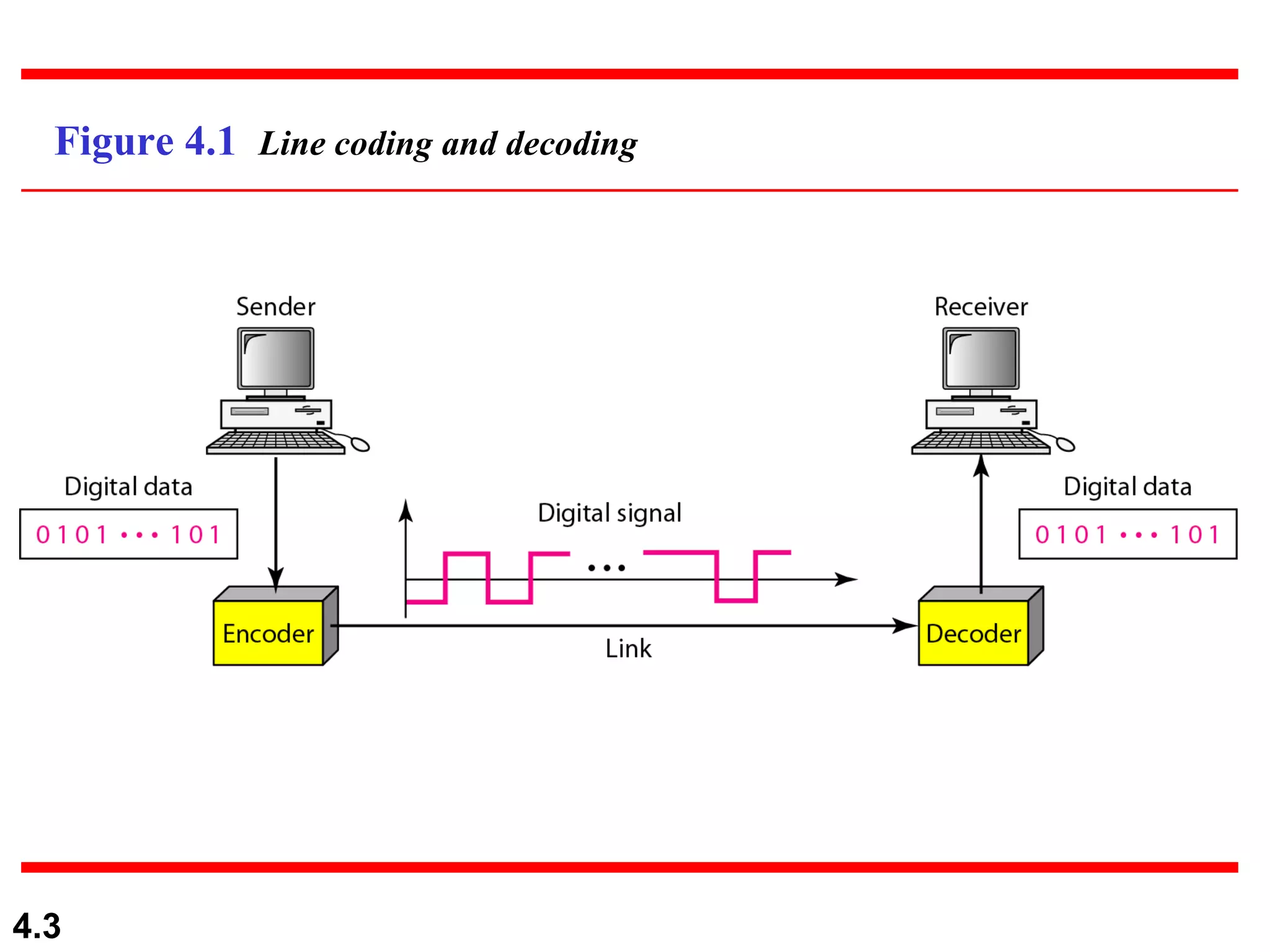
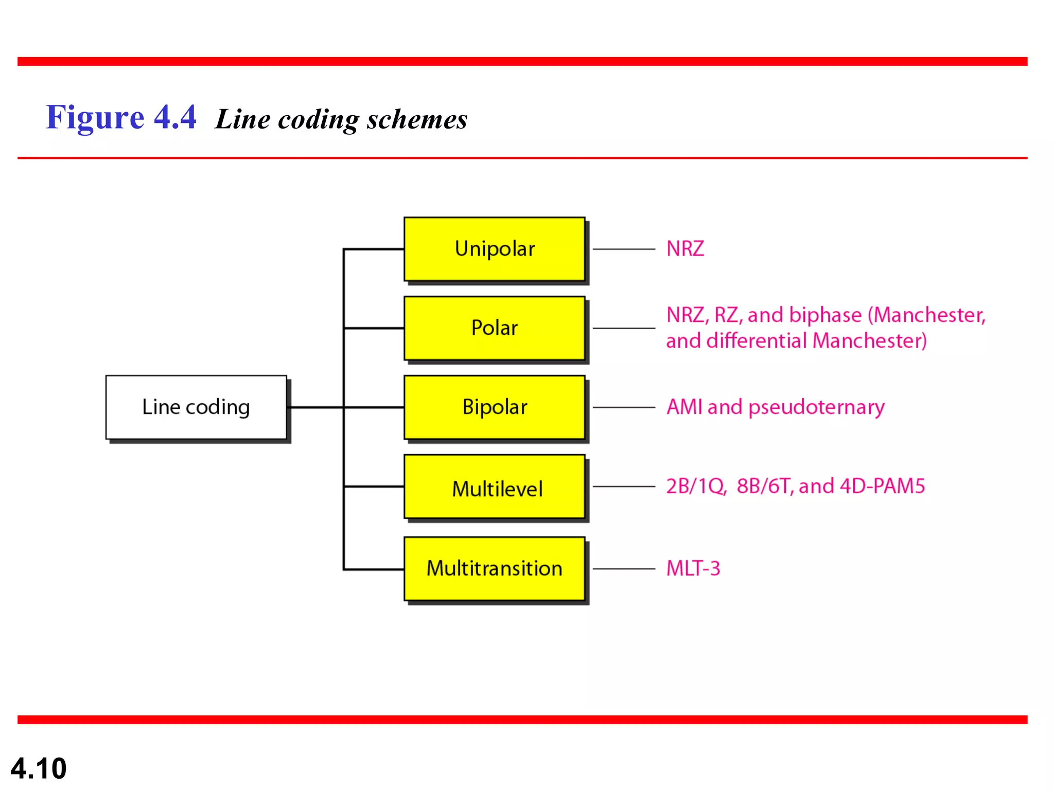
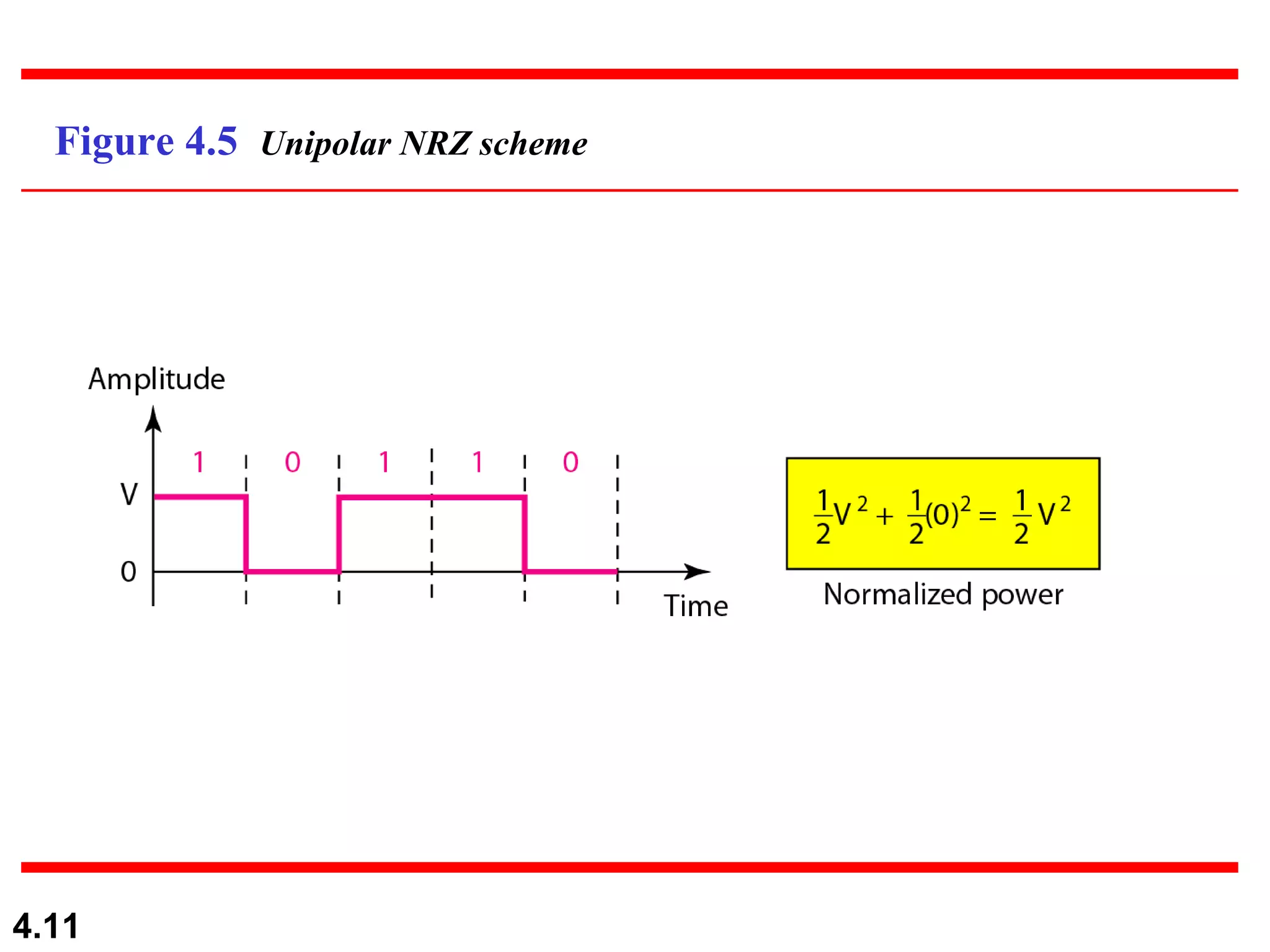
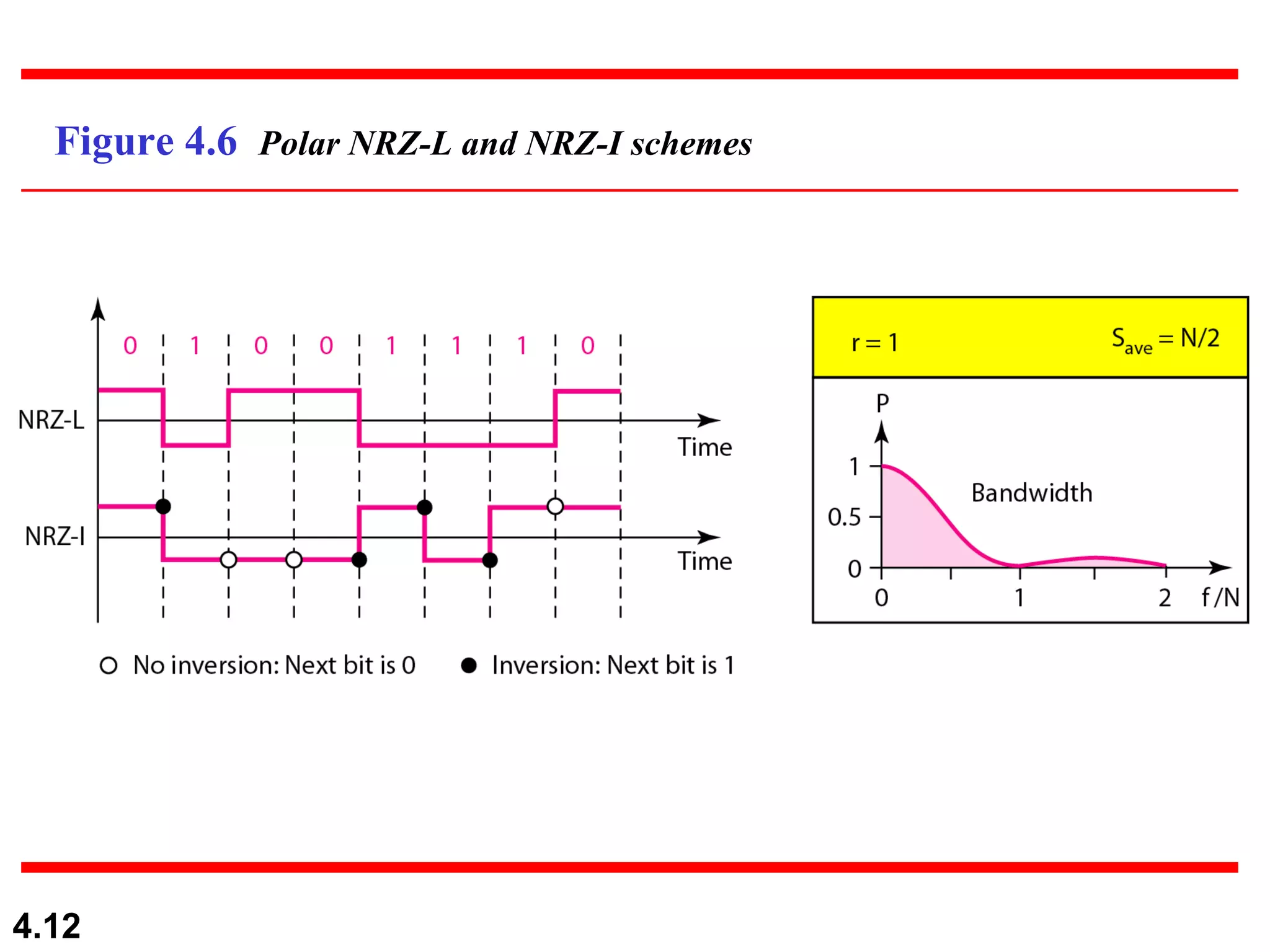
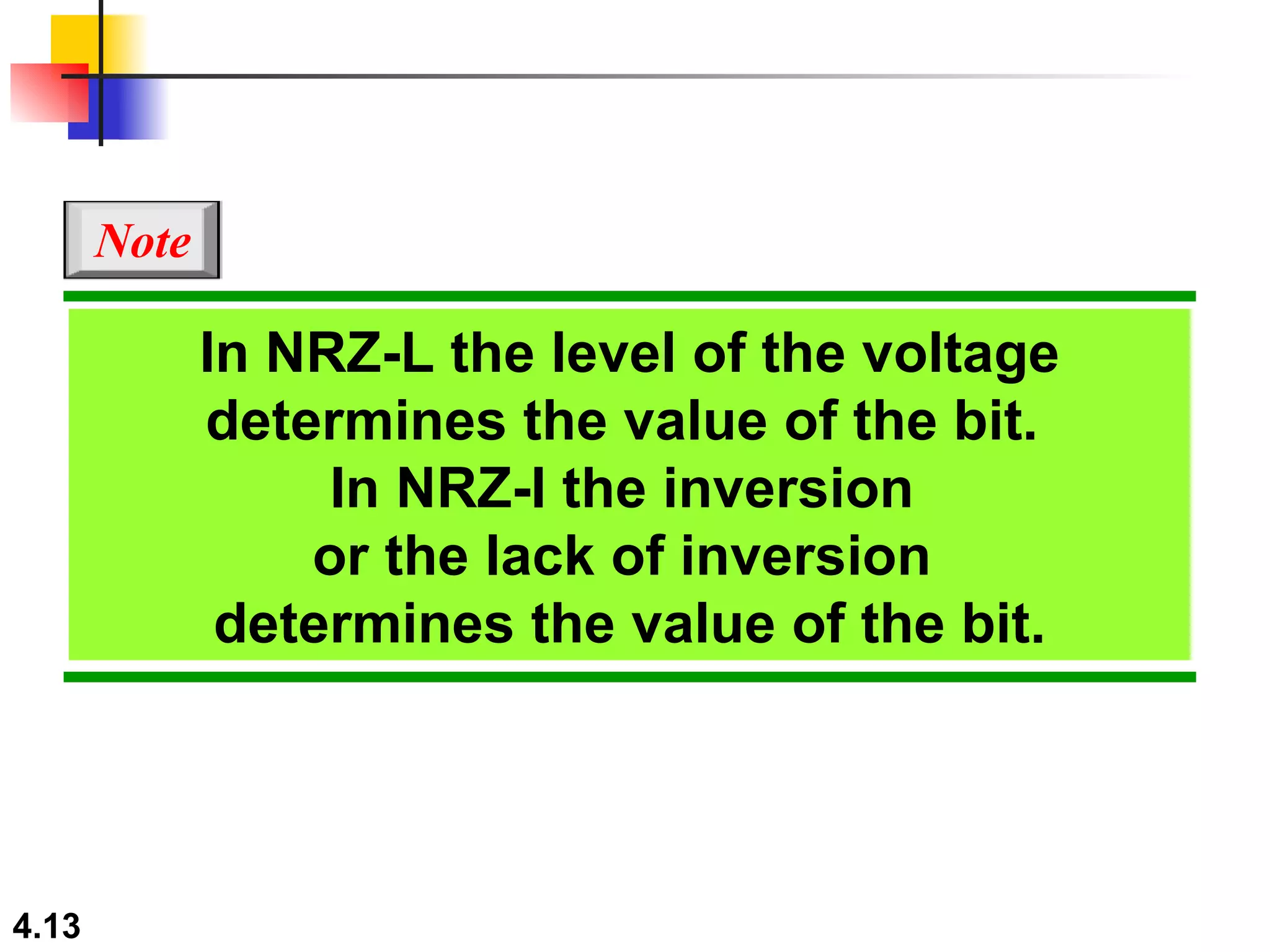
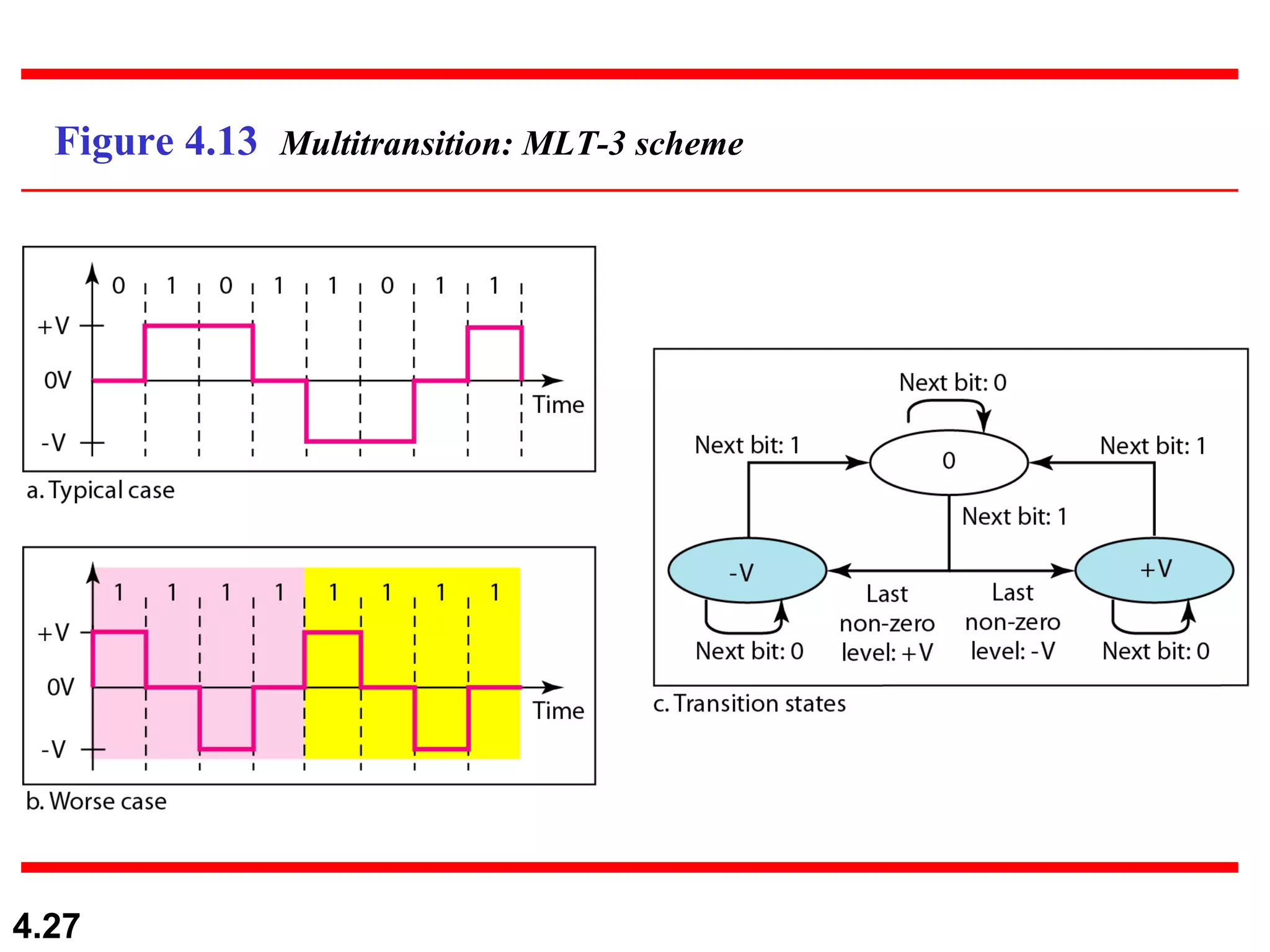
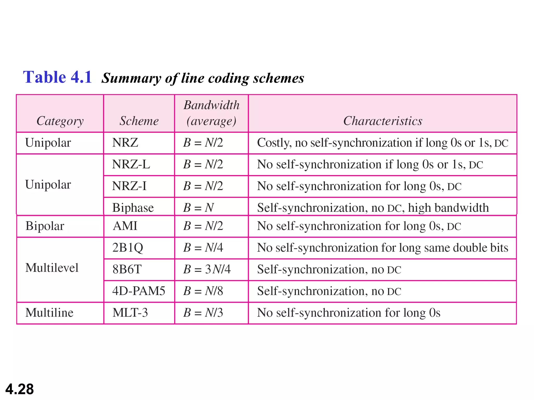
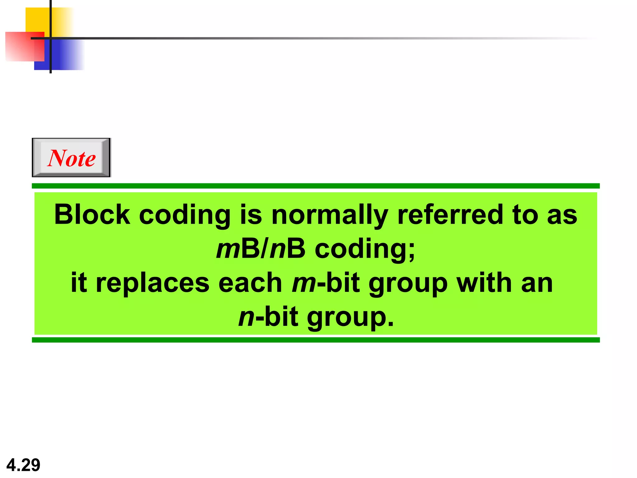
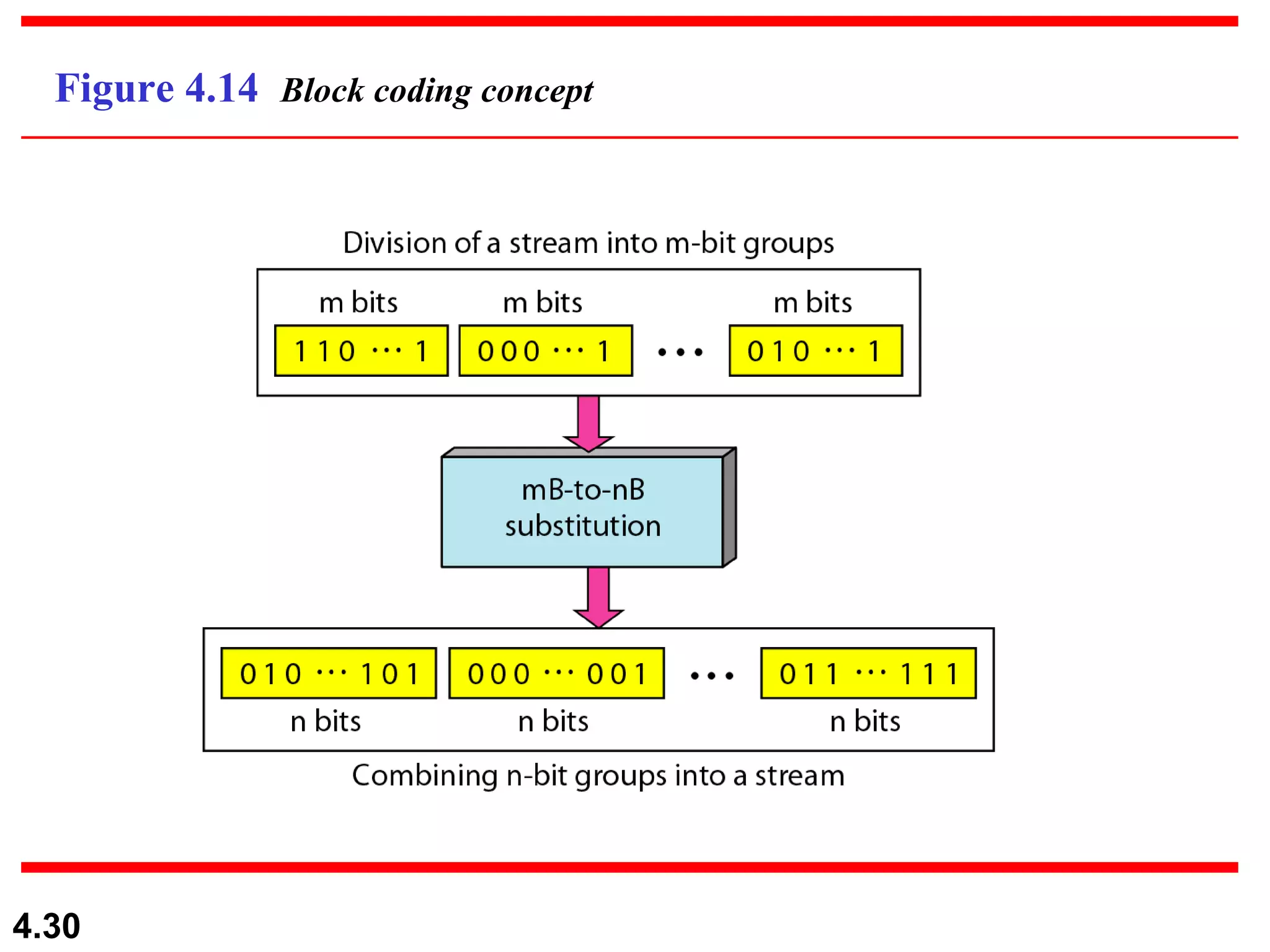
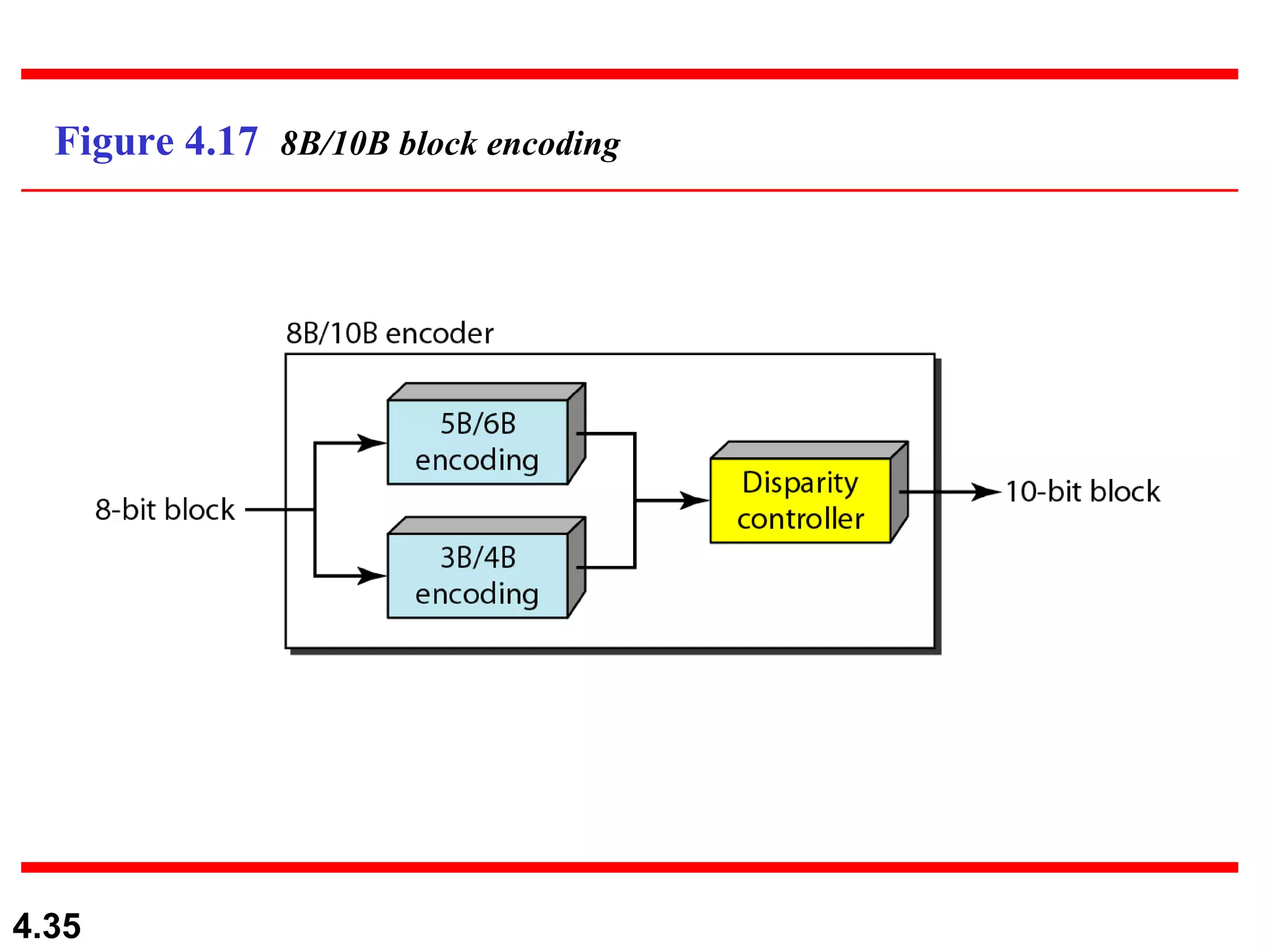
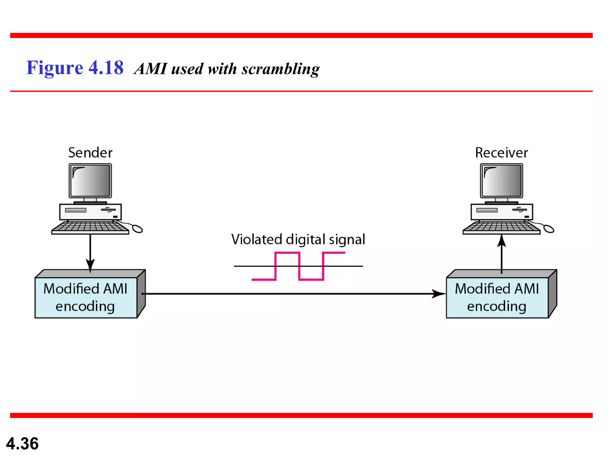
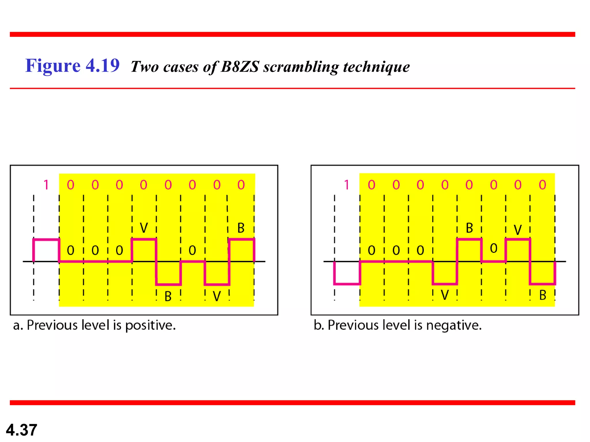
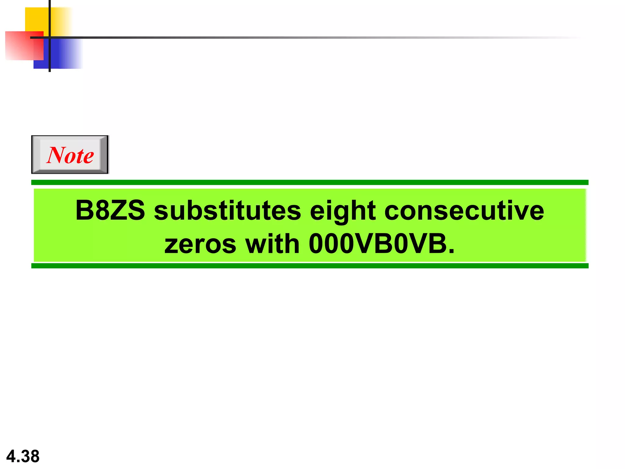
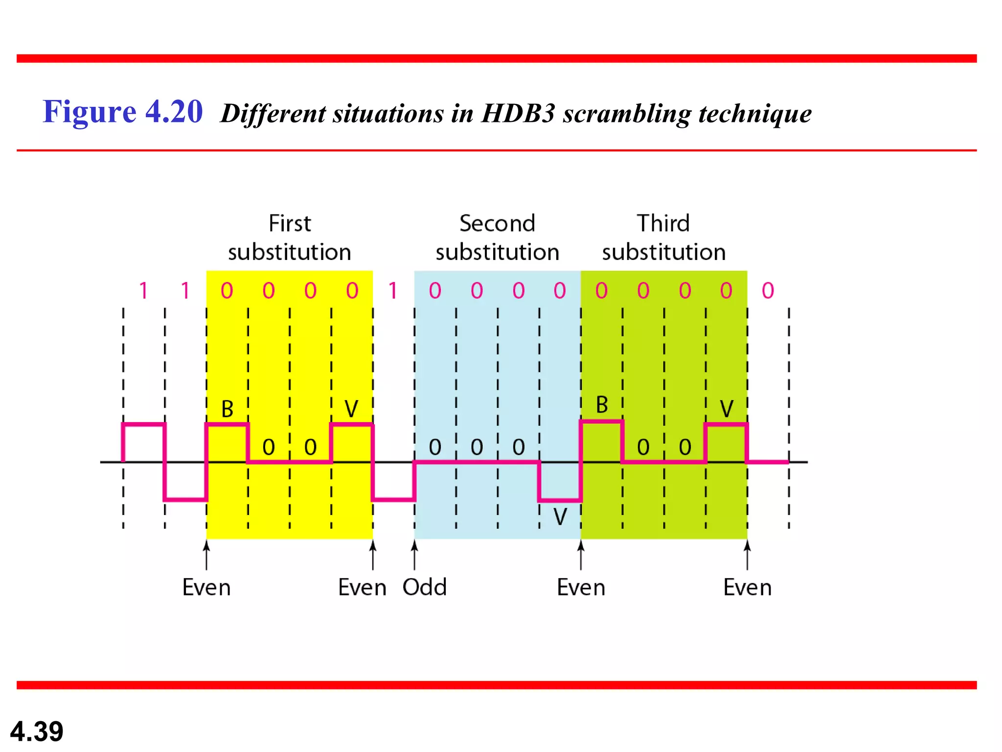
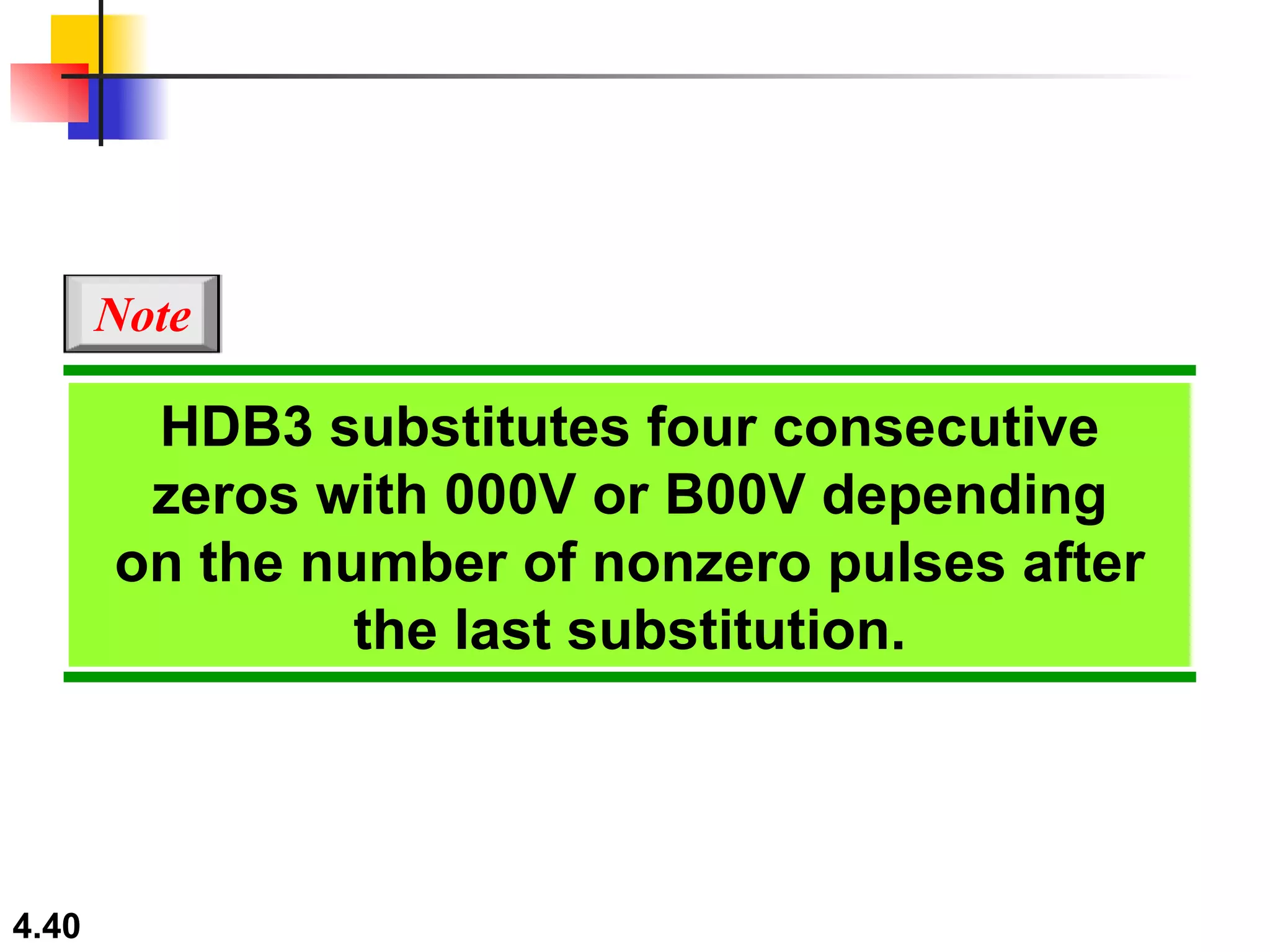
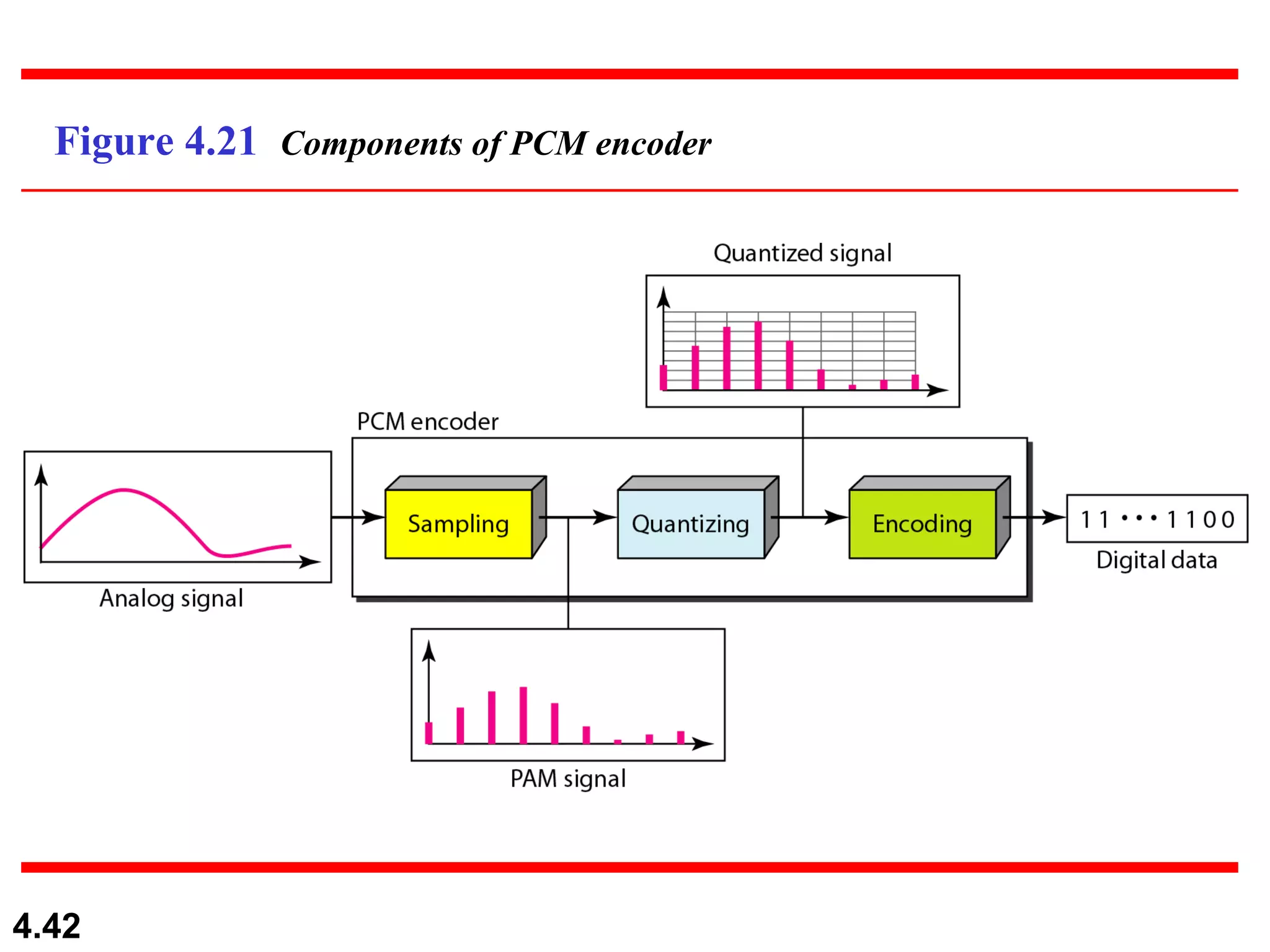
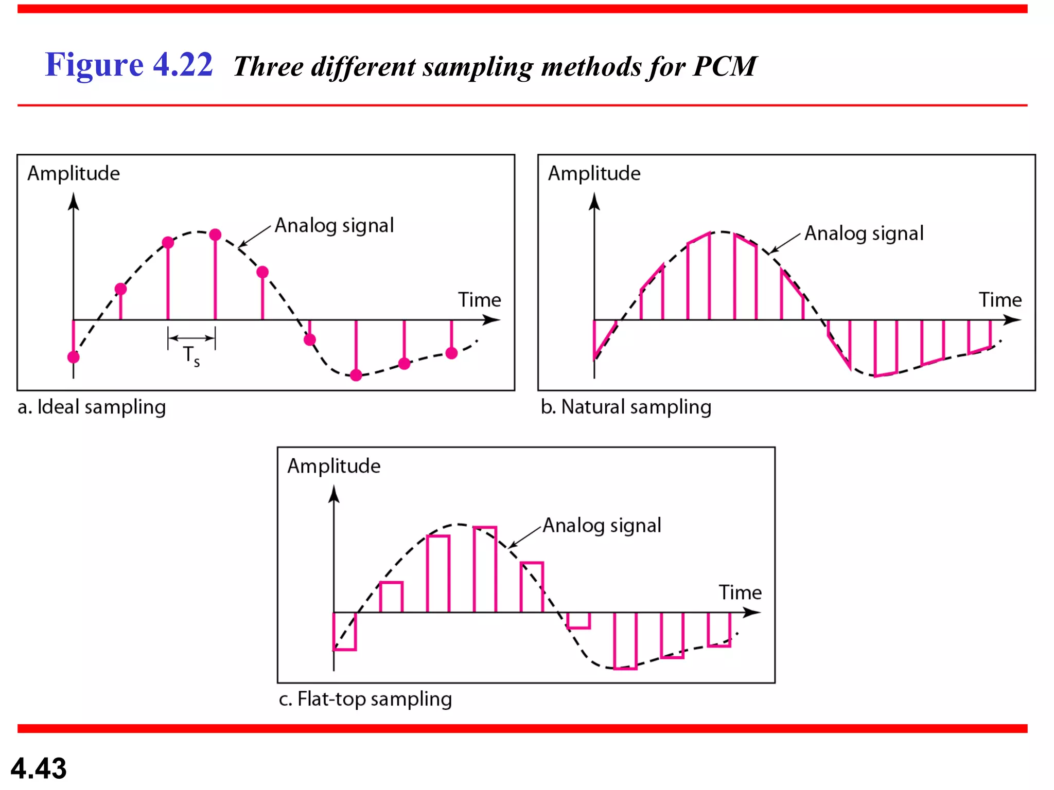
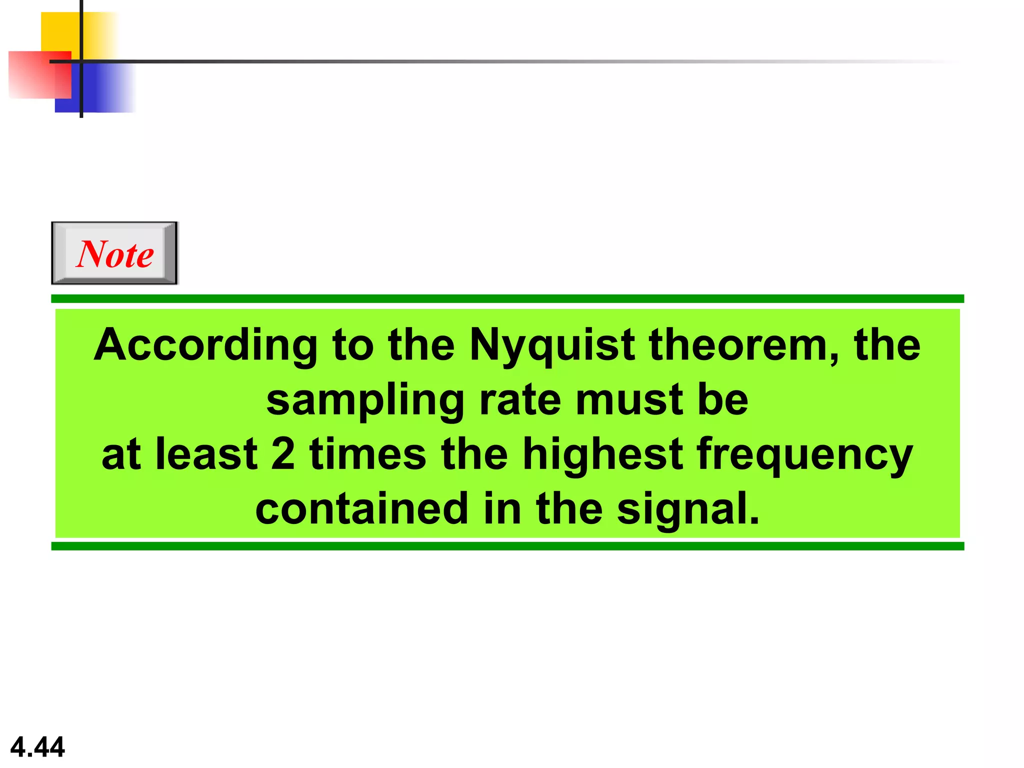
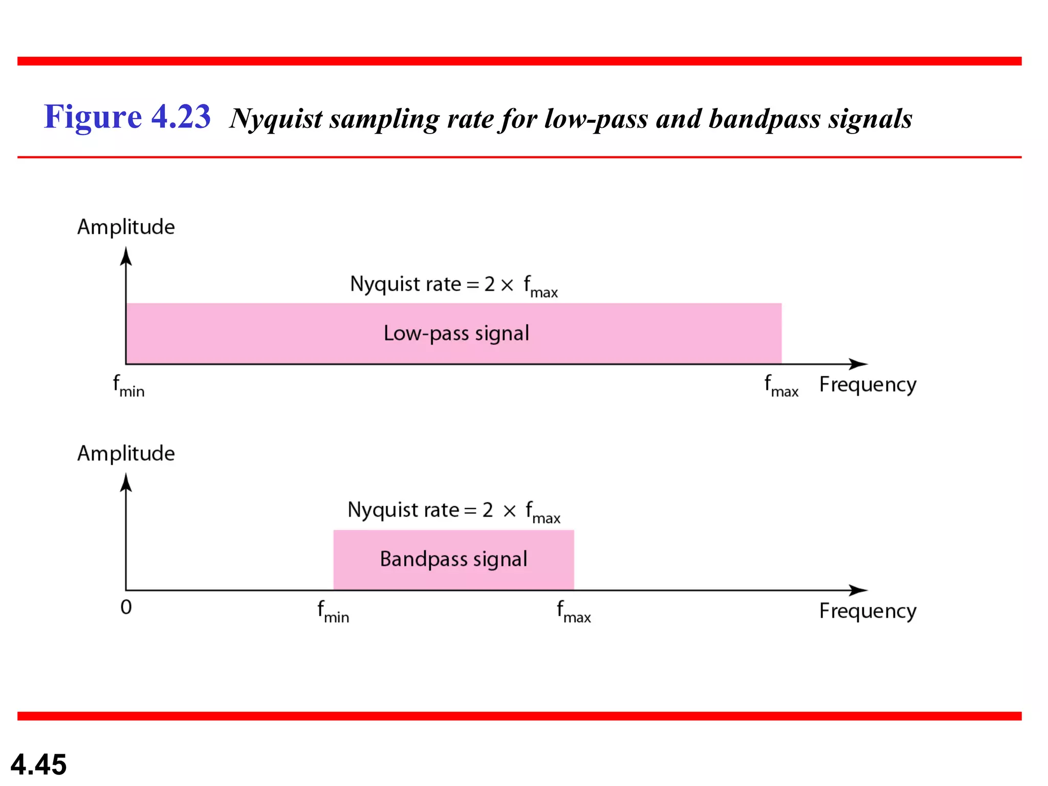
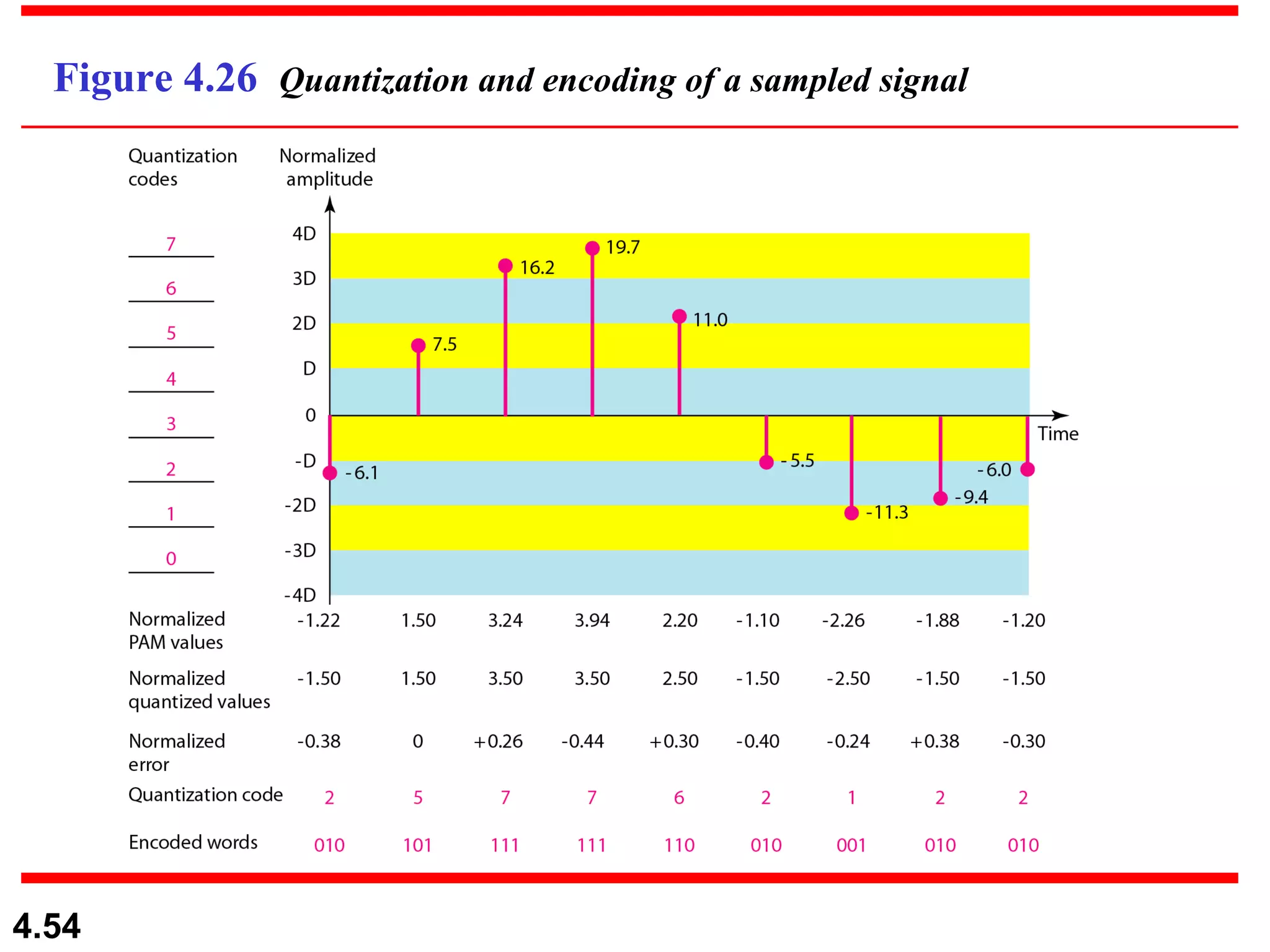
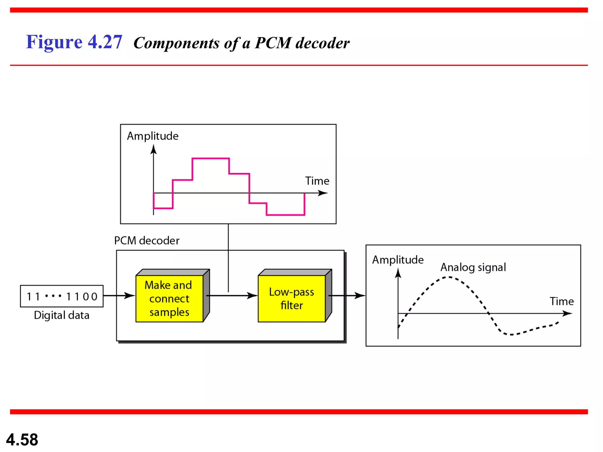
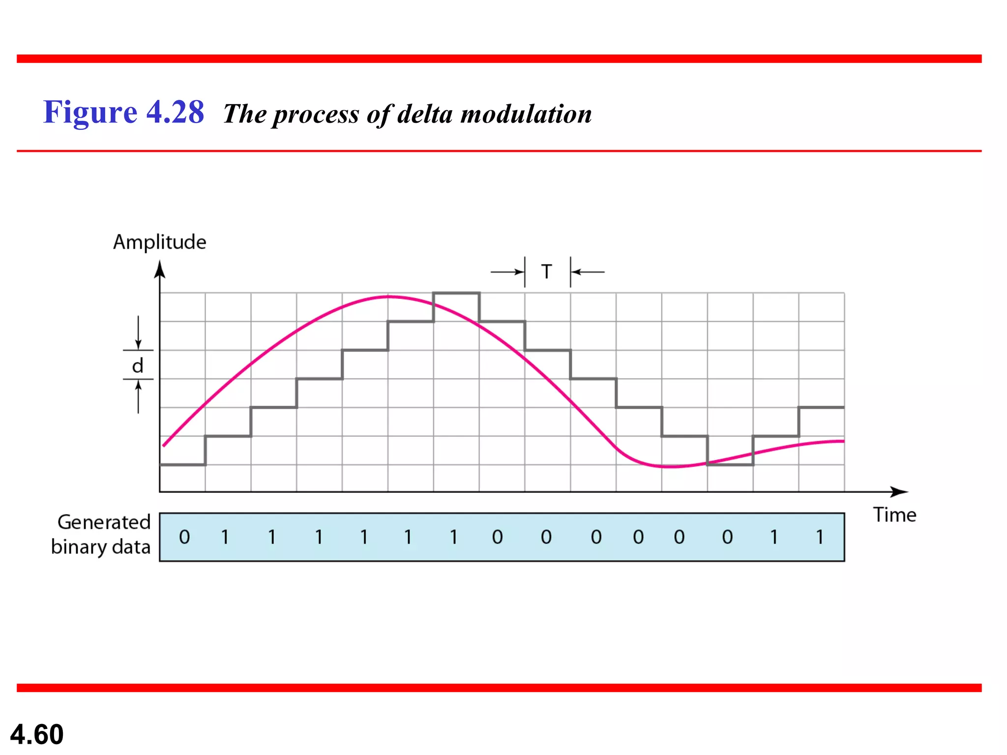
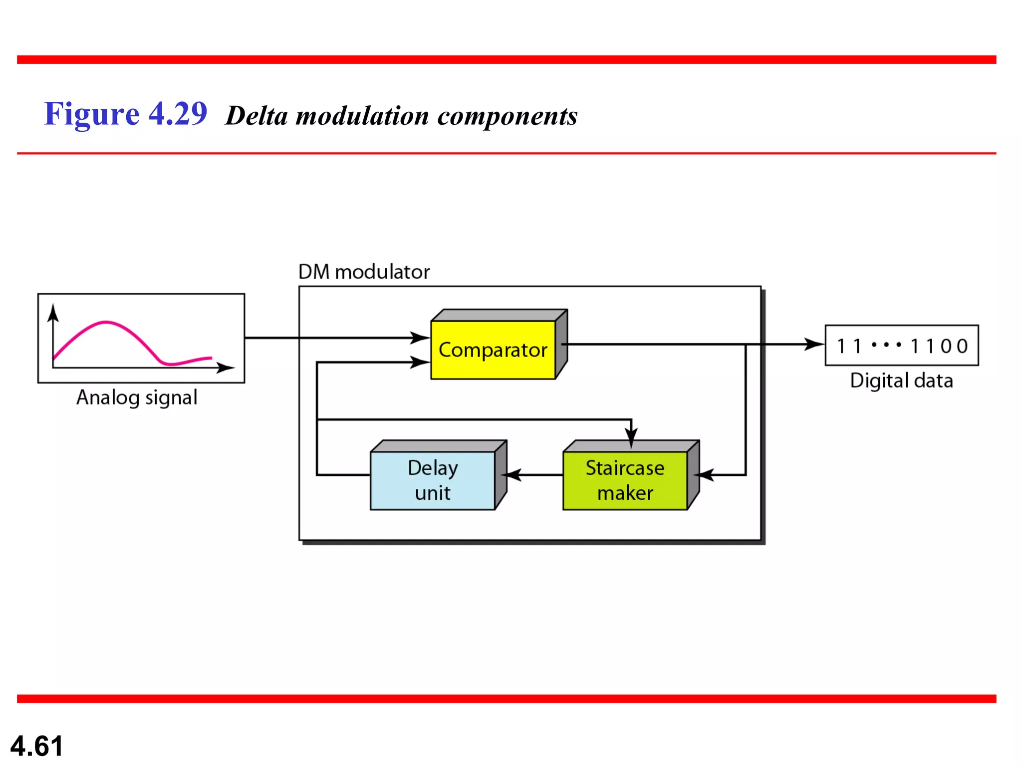
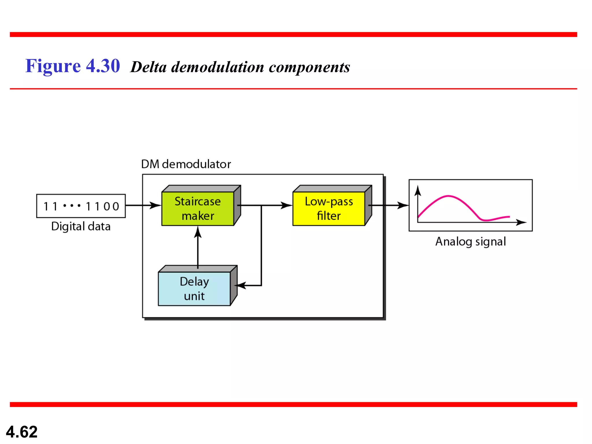
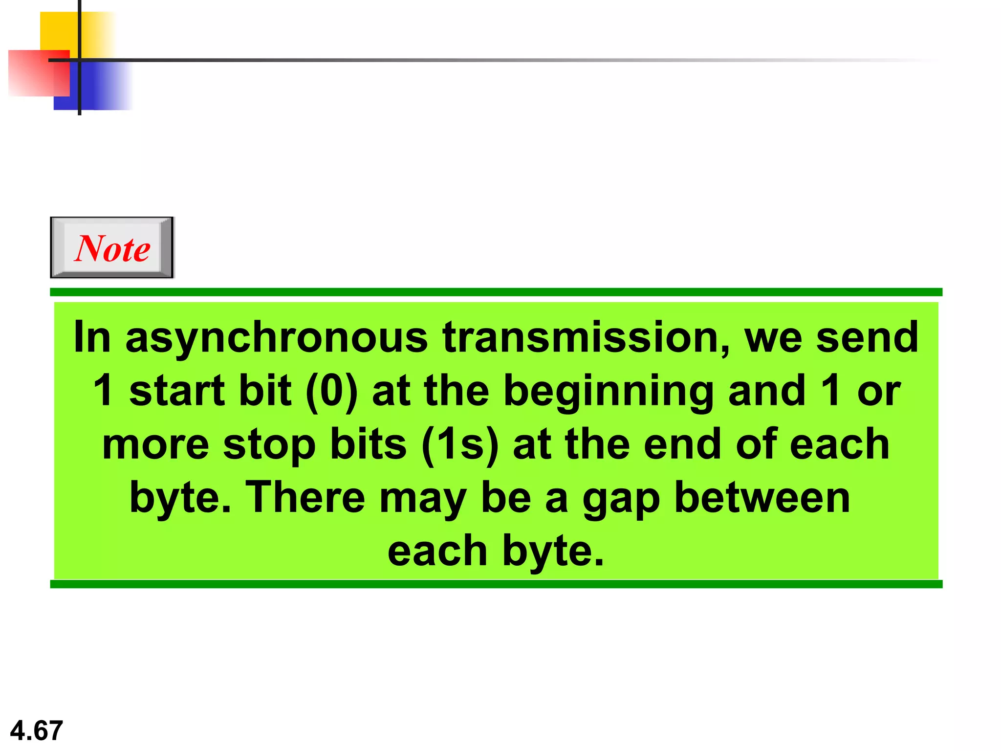
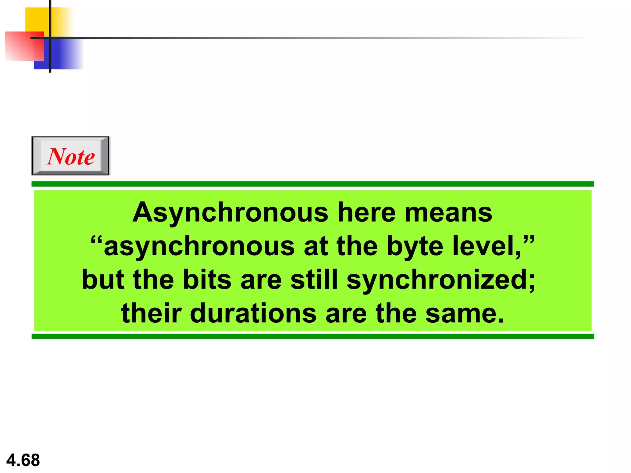
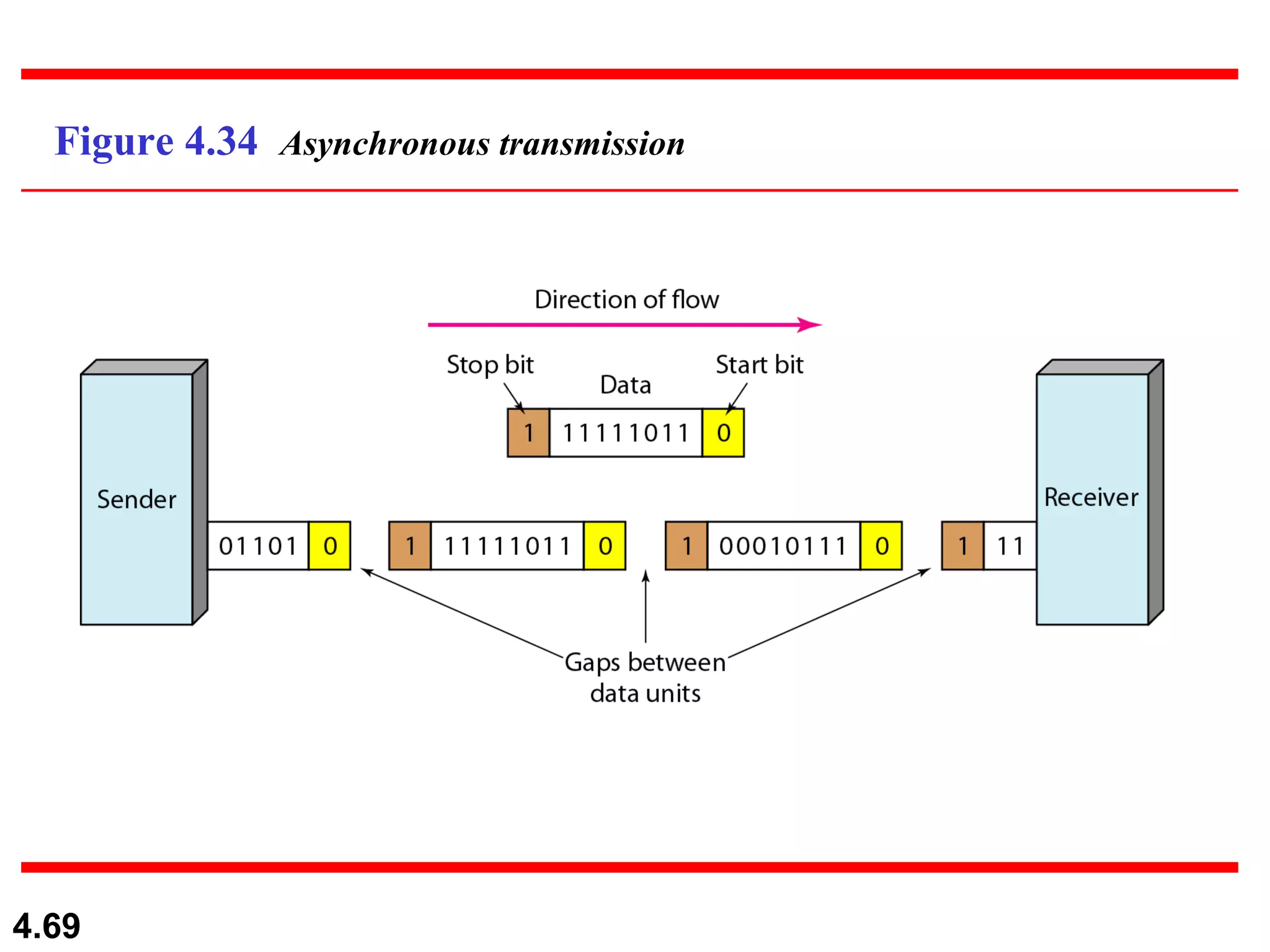
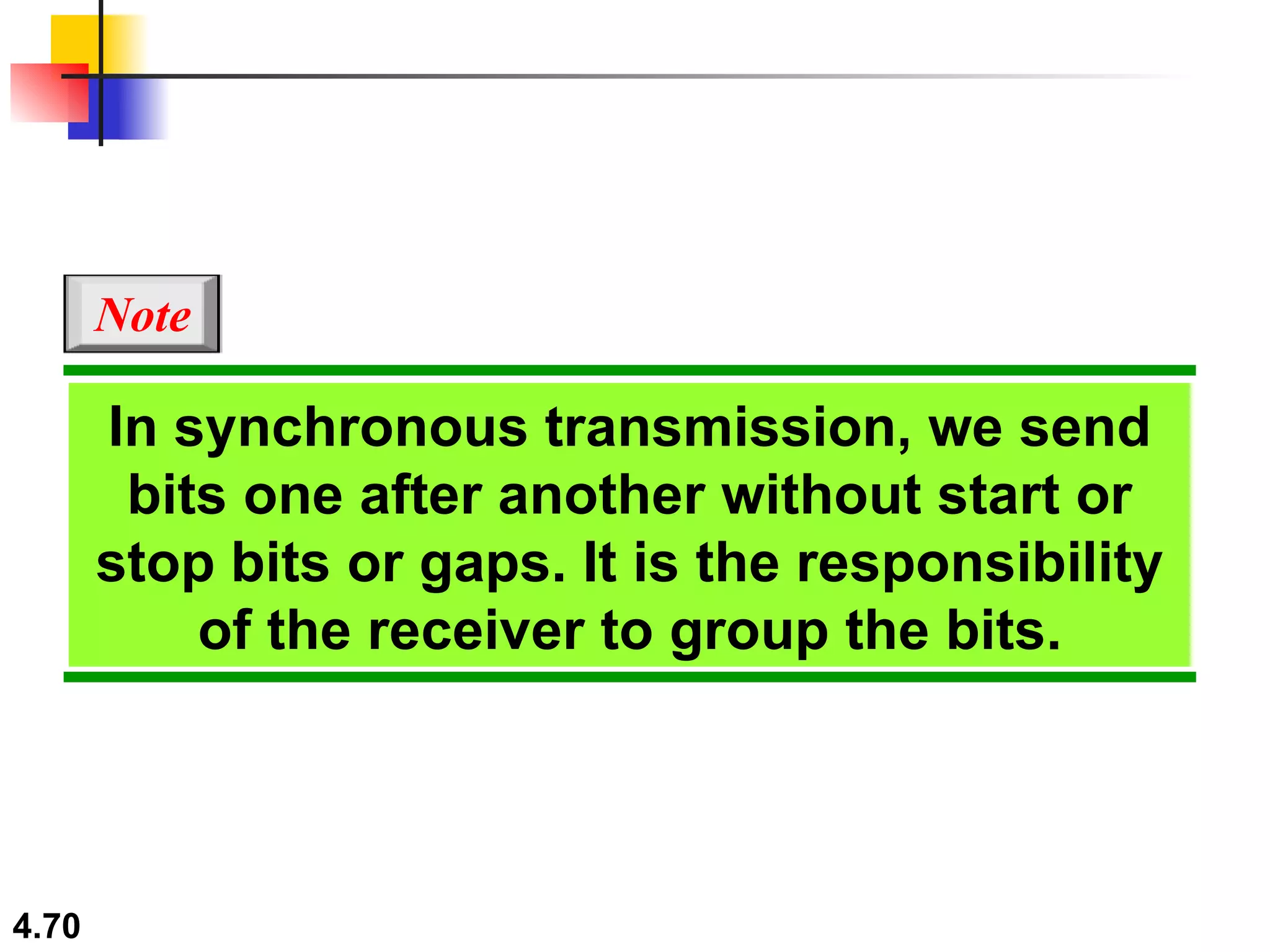
Chapter 4 Digital Transmission Copyright © The McGraw-Hill Companies, Inc. Permission required for reproduction or display.
4-1  DIGITAL-TO-DIGITAL CONVERSION In this section, we see how we can represent digital data by using digital signals. The conversion involves three techniques:  line coding ,  block coding , and  scrambling . Line coding is always needed; block coding and scrambling may or may not be needed. Line Coding Line Coding Schemes Block Coding Scrambling Topics discussed in this section:
Figure 4.1  Line coding and decoding
Figure 4.2  Signal element versus data element
A signal is carrying data in which one data element is encoded as one signal element ( r = 1). If the bit rate is 100 kbps, what is the average value of the baud rate if c is between 0 and 1? Solution We assume that the average value of c is 1/2 . The baud rate is then Example 4.1
Although the actual bandwidth of a digital signal is infinite, the effective bandwidth is finite. Note
The maximum data rate of a channel (see Chapter 3) is N max  = 2 × B × log 2  L (defined by the Nyquist formula). Does this agree with the previous formula for N max ? Solution A signal with L levels actually can carry log 2 L bits per level. If each level corresponds to one signal element and we assume the average case (c = 1/2), then we have Example 4.2
Figure 4.3  Effect of lack of synchronization
In a digital transmission, the receiver clock is 0.1 percent faster than the sender clock. How many extra bits per second does the receiver receive if the data rate is  1 kbps? How many if the data rate is 1 Mbps? Solution At 1 kbps, the receiver receives 1001 bps instead of 1000 bps. Example 4.3 At 1 Mbps, the receiver receives 1,001,000 bps instead of 1,000,000 bps.
Figure 4.4  Line coding schemes
Figure 4.5  Unipolar NRZ scheme
Figure 4.6  Polar NRZ-L and NRZ-I schemes
In NRZ-L the level of the voltage determines the value of the bit.  In NRZ-I the inversion  or the lack of inversion  determines the value of the bit. Note
NRZ-L and NRZ-I both have an average signal rate of N/2 Bd. Note
NRZ-L and NRZ-I both have a DC component problem. Note
A system is using NRZ-I to transfer 10-Mbps data. What are the average signal rate and minimum bandwidth? Solution The average signal rate is S = N/2 = 500 kbaud. The minimum bandwidth for this average baud rate is B min  = S = 500 kHz. Example 4.4
Figure 4.7  Polar RZ scheme
Figure 4.8  Polar biphase: Manchester and differential Manchester schemes
In Manchester and differential Manchester encoding, the transition at the middle of the bit is used for synchronization. Note
The minimum bandwidth of Manchester and differential Manchester is 2 times that of NRZ. Note
In bipolar encoding, we use three levels: positive, zero, and negative. Note
Figure 4.9  Bipolar schemes: AMI and pseudoternary
In  m B n L schemes, a pattern of  m  data elements is encoded as a pattern of  n  signal elements in which 2 m  ≤ L n . Note
Figure 4.10  Multilevel: 2B1Q scheme
Figure 4.11  Multilevel: 8B6T scheme
Figure 4.12  Multilevel: 4D-PAM5 scheme
Figure 4.13  Multitransition: MLT-3 scheme
Table 4.1  Summary of line coding schemes
Block coding is normally referred to as  m B/ n B coding; it replaces each  m -bit group with an  n -bit group. Note
Figure 4.14  Block coding concept
Figure 4.15  Using block coding 4B/5B with NRZ-I line coding scheme
Table 4.2  4B/5B mapping codes
Figure 4.16  Substitution in 4B/5B block coding
We need to send data at a 1-Mbps rate. What is the minimum required bandwidth, using a combination of 4B/5B and NRZ-I or Manchester coding? Solution First 4B/5B block coding increases the bit rate to 1.25 Mbps. The minimum bandwidth using NRZ-I is N/2 or 625 kHz. The Manchester scheme needs a minimum bandwidth of 1 MHz. The first choice needs a lower bandwidth, but has a DC component problem; the second choice needs a higher bandwidth, but does not have a DC component problem. Example 4.5
Figure 4.17  8B/10B block encoding
Figure 4.18  AMI used with scrambling
Figure 4.19  Two cases of B8ZS scrambling technique
B8ZS substitutes eight consecutive zeros with 000VB0VB. Note
Figure 4.20  Different situations in HDB3 scrambling technique
HDB3 substitutes four consecutive zeros with 000V or B00V depending on the number of nonzero pulses after the last substitution. Note
4-2  ANALOG-TO-DIGITAL CONVERSION We have seen in Chapter 3 that a digital signal is superior to an analog signal. The tendency today is to change an analog signal to digital data. In this section we describe two techniques,  pulse code modulation  and  delta modulation .  Pulse Code Modulation (PCM) Delta Modulation (DM) Topics discussed in this section:
Figure 4.21  Components of PCM encoder
Figure 4.22  Three different sampling methods for PCM
According to the Nyquist theorem, the sampling rate must be at least 2 times the highest frequency contained in the signal. Note
Figure 4.23  Nyquist sampling rate for low-pass and bandpass signals
For an intuitive example of the Nyquist theorem, let us sample a simple sine wave at three sampling rates: f s  = 4f (2 times the Nyquist rate), f s  = 2f (Nyquist rate), and  f s  = f (one-half the Nyquist rate). Figure 4.24 shows the sampling and the subsequent recovery of the signal. It can be seen that sampling at the Nyquist rate can create a good approximation of the original sine wave (part a). Oversampling in part b can also create the same approximation, but it is redundant and unnecessary. Sampling below the Nyquist rate (part c) does not produce a signal that looks like the original sine wave. Example 4.6
Figure 4.24  Recovery of a sampled sine wave for different sampling rates
Consider the revolution of a hand of a clock. The second hand of a clock has a period of 60 s. According to the Nyquist theorem, we need to sample the hand every 30 s (T s  = T or f s  = 2f ). In Figure 4.25a, the sample points, in order, are 12, 6, 12, 6, 12, and 6. The receiver of the samples cannot tell if the clock is moving forward or backward. In part b, we sample at double the Nyquist rate (every 15 s). The sample points are 12, 3, 6, 9, and 12. The clock is moving forward. In part c, we sample below the Nyquist rate (T s  = T or f s  = f ). The sample points are 12, 9, 6, 3, and 12. Although the clock is moving forward, the receiver thinks that the clock is moving backward. Example 4.7
Figure 4.25  Sampling of a clock with only one hand
An example related to Example 4.7 is the seemingly backward rotation of the wheels of a forward-moving car in a movie. This can be explained by under-sampling. A movie is filmed at 24 frames per second. If a wheel is rotating more than 12 times per second, the under-sampling creates the impression of a backward rotation. Example 4.8
Telephone companies digitize voice by assuming a maximum frequency of 4000 Hz. The sampling rate therefore is 8000 samples per second. Example 4.9
A complex low-pass signal has a bandwidth of 200 kHz. What is the minimum sampling rate for this signal? Solution The bandwidth of a low-pass signal is between 0 and f, where f is the maximum frequency in the signal. Therefore, we can sample this signal at 2 times the highest frequency (200 kHz). The sampling rate is therefore 400,000 samples per second. Example 4.10
A complex bandpass signal has a bandwidth of 200 kHz. What is the minimum sampling rate for this signal? Solution We cannot find the minimum sampling rate in this case because we do not know where the bandwidth starts or ends. We do not know the maximum frequency in the signal. Example 4.11
Figure 4.26  Quantization and encoding of a sampled signal
What is the SNR dB  in the example of Figure 4.26? Solution We can use the formula to find the quantization. We have eight levels and 3 bits per sample, so  SNR dB  = 6.02(3) + 1.76 = 19.82 dB   Increasing the number of levels increases the SNR. Example 4.12
A telephone subscriber line must have an SNR dB  above 40. What is the minimum number of bits per sample? Solution We can calculate the number of bits as Example 4.13 Telephone companies usually assign 7 or 8 bits per sample.
We want to digitize the human voice. What is the bit rate, assuming 8 bits per sample? Solution The human voice normally contains frequencies from 0 to 4000 Hz. So the sampling rate and bit rate are calculated as follows: Example 4.14
Figure 4.27  Components of a PCM decoder
We have a low-pass analog signal of 4 kHz. If we send the analog signal, we need a channel with a minimum bandwidth of 4 kHz. If we digitize the signal and send 8 bits per sample, we need a channel with a minimum bandwidth of 8 × 4 kHz = 32 kHz. Example 4.15
Figure 4.28  The process of delta modulation
Figure 4.29  Delta modulation components
Figure 4.30  Delta demodulation components
4-3  TRANSMISSION MODES The transmission of binary data across a link can be accomplished in either parallel or serial mode. In parallel mode, multiple bits are sent with each clock tick. In serial mode, 1 bit is sent with each clock tick. While there is only one way to send parallel data, there are three subclasses of serial transmission: asynchronous, synchronous, and isochronous. Parallel Transmission Serial Transmission Topics discussed in this section:
Figure 4.31  Data transmission and modes
Figure 4.32  Parallel transmission
Figure 4.33  Serial transmission
In asynchronous transmission, we send 1 start bit (0) at the beginning and 1 or more stop bits (1s) at the end of each byte. There may be a gap between  each byte. Note
Asynchronous here means “asynchronous at the byte level,” but the bits are still synchronized;  their durations are the same. Note
Figure 4.34  Asynchronous transmission
In synchronous transmission, we send bits one after another without start or stop bits or gaps. It is the responsibility of the receiver to group the bits. Note
Figure 4.35  Synchronous transmission

Ch04

  • 1.
    Chapter 4 DigitalTransmission Copyright © The McGraw-Hill Companies, Inc. Permission required for reproduction or display.
  • 2.
    4-1 DIGITAL-TO-DIGITALCONVERSION In this section, we see how we can represent digital data by using digital signals. The conversion involves three techniques: line coding , block coding , and scrambling . Line coding is always needed; block coding and scrambling may or may not be needed. Line Coding Line Coding Schemes Block Coding Scrambling Topics discussed in this section:
  • 3.
    Figure 4.1 Line coding and decoding
  • 4.
    Figure 4.2 Signal element versus data element
  • 5.
    A signal iscarrying data in which one data element is encoded as one signal element ( r = 1). If the bit rate is 100 kbps, what is the average value of the baud rate if c is between 0 and 1? Solution We assume that the average value of c is 1/2 . The baud rate is then Example 4.1
  • 6.
    Although the actualbandwidth of a digital signal is infinite, the effective bandwidth is finite. Note
  • 7.
    The maximum datarate of a channel (see Chapter 3) is N max = 2 × B × log 2 L (defined by the Nyquist formula). Does this agree with the previous formula for N max ? Solution A signal with L levels actually can carry log 2 L bits per level. If each level corresponds to one signal element and we assume the average case (c = 1/2), then we have Example 4.2
  • 8.
    Figure 4.3 Effect of lack of synchronization
  • 9.
    In a digitaltransmission, the receiver clock is 0.1 percent faster than the sender clock. How many extra bits per second does the receiver receive if the data rate is 1 kbps? How many if the data rate is 1 Mbps? Solution At 1 kbps, the receiver receives 1001 bps instead of 1000 bps. Example 4.3 At 1 Mbps, the receiver receives 1,001,000 bps instead of 1,000,000 bps.
  • 10.
    Figure 4.4 Line coding schemes
  • 11.
    Figure 4.5 Unipolar NRZ scheme
  • 12.
    Figure 4.6 Polar NRZ-L and NRZ-I schemes
  • 13.
    In NRZ-L thelevel of the voltage determines the value of the bit. In NRZ-I the inversion or the lack of inversion determines the value of the bit. Note
  • 14.
    NRZ-L and NRZ-Iboth have an average signal rate of N/2 Bd. Note
  • 15.
    NRZ-L and NRZ-Iboth have a DC component problem. Note
  • 16.
    A system isusing NRZ-I to transfer 10-Mbps data. What are the average signal rate and minimum bandwidth? Solution The average signal rate is S = N/2 = 500 kbaud. The minimum bandwidth for this average baud rate is B min = S = 500 kHz. Example 4.4
  • 17.
    Figure 4.7 Polar RZ scheme
  • 18.
    Figure 4.8 Polar biphase: Manchester and differential Manchester schemes
  • 19.
    In Manchester anddifferential Manchester encoding, the transition at the middle of the bit is used for synchronization. Note
  • 20.
    The minimum bandwidthof Manchester and differential Manchester is 2 times that of NRZ. Note
  • 21.
    In bipolar encoding,we use three levels: positive, zero, and negative. Note
  • 22.
    Figure 4.9 Bipolar schemes: AMI and pseudoternary
  • 23.
    In mB n L schemes, a pattern of m data elements is encoded as a pattern of n signal elements in which 2 m ≤ L n . Note
  • 24.
    Figure 4.10 Multilevel: 2B1Q scheme
  • 25.
    Figure 4.11 Multilevel: 8B6T scheme
  • 26.
    Figure 4.12 Multilevel: 4D-PAM5 scheme
  • 27.
    Figure 4.13 Multitransition: MLT-3 scheme
  • 28.
    Table 4.1 Summary of line coding schemes
  • 29.
    Block coding isnormally referred to as m B/ n B coding; it replaces each m -bit group with an n -bit group. Note
  • 30.
    Figure 4.14 Block coding concept
  • 31.
    Figure 4.15 Using block coding 4B/5B with NRZ-I line coding scheme
  • 32.
    Table 4.2 4B/5B mapping codes
  • 33.
    Figure 4.16 Substitution in 4B/5B block coding
  • 34.
    We need tosend data at a 1-Mbps rate. What is the minimum required bandwidth, using a combination of 4B/5B and NRZ-I or Manchester coding? Solution First 4B/5B block coding increases the bit rate to 1.25 Mbps. The minimum bandwidth using NRZ-I is N/2 or 625 kHz. The Manchester scheme needs a minimum bandwidth of 1 MHz. The first choice needs a lower bandwidth, but has a DC component problem; the second choice needs a higher bandwidth, but does not have a DC component problem. Example 4.5
  • 35.
    Figure 4.17 8B/10B block encoding
  • 36.
    Figure 4.18 AMI used with scrambling
  • 37.
    Figure 4.19 Two cases of B8ZS scrambling technique
  • 38.
    B8ZS substitutes eightconsecutive zeros with 000VB0VB. Note
  • 39.
    Figure 4.20 Different situations in HDB3 scrambling technique
  • 40.
    HDB3 substitutes fourconsecutive zeros with 000V or B00V depending on the number of nonzero pulses after the last substitution. Note
  • 41.
    4-2 ANALOG-TO-DIGITALCONVERSION We have seen in Chapter 3 that a digital signal is superior to an analog signal. The tendency today is to change an analog signal to digital data. In this section we describe two techniques, pulse code modulation and delta modulation . Pulse Code Modulation (PCM) Delta Modulation (DM) Topics discussed in this section:
  • 42.
    Figure 4.21 Components of PCM encoder
  • 43.
    Figure 4.22 Three different sampling methods for PCM
  • 44.
    According to theNyquist theorem, the sampling rate must be at least 2 times the highest frequency contained in the signal. Note
  • 45.
    Figure 4.23 Nyquist sampling rate for low-pass and bandpass signals
  • 46.
    For an intuitiveexample of the Nyquist theorem, let us sample a simple sine wave at three sampling rates: f s = 4f (2 times the Nyquist rate), f s = 2f (Nyquist rate), and f s = f (one-half the Nyquist rate). Figure 4.24 shows the sampling and the subsequent recovery of the signal. It can be seen that sampling at the Nyquist rate can create a good approximation of the original sine wave (part a). Oversampling in part b can also create the same approximation, but it is redundant and unnecessary. Sampling below the Nyquist rate (part c) does not produce a signal that looks like the original sine wave. Example 4.6
  • 47.
    Figure 4.24 Recovery of a sampled sine wave for different sampling rates
  • 48.
    Consider the revolutionof a hand of a clock. The second hand of a clock has a period of 60 s. According to the Nyquist theorem, we need to sample the hand every 30 s (T s = T or f s = 2f ). In Figure 4.25a, the sample points, in order, are 12, 6, 12, 6, 12, and 6. The receiver of the samples cannot tell if the clock is moving forward or backward. In part b, we sample at double the Nyquist rate (every 15 s). The sample points are 12, 3, 6, 9, and 12. The clock is moving forward. In part c, we sample below the Nyquist rate (T s = T or f s = f ). The sample points are 12, 9, 6, 3, and 12. Although the clock is moving forward, the receiver thinks that the clock is moving backward. Example 4.7
  • 49.
    Figure 4.25 Sampling of a clock with only one hand
  • 50.
    An example relatedto Example 4.7 is the seemingly backward rotation of the wheels of a forward-moving car in a movie. This can be explained by under-sampling. A movie is filmed at 24 frames per second. If a wheel is rotating more than 12 times per second, the under-sampling creates the impression of a backward rotation. Example 4.8
  • 51.
    Telephone companies digitizevoice by assuming a maximum frequency of 4000 Hz. The sampling rate therefore is 8000 samples per second. Example 4.9
  • 52.
    A complex low-passsignal has a bandwidth of 200 kHz. What is the minimum sampling rate for this signal? Solution The bandwidth of a low-pass signal is between 0 and f, where f is the maximum frequency in the signal. Therefore, we can sample this signal at 2 times the highest frequency (200 kHz). The sampling rate is therefore 400,000 samples per second. Example 4.10
  • 53.
    A complex bandpasssignal has a bandwidth of 200 kHz. What is the minimum sampling rate for this signal? Solution We cannot find the minimum sampling rate in this case because we do not know where the bandwidth starts or ends. We do not know the maximum frequency in the signal. Example 4.11
  • 54.
    Figure 4.26 Quantization and encoding of a sampled signal
  • 55.
    What is theSNR dB in the example of Figure 4.26? Solution We can use the formula to find the quantization. We have eight levels and 3 bits per sample, so SNR dB = 6.02(3) + 1.76 = 19.82 dB Increasing the number of levels increases the SNR. Example 4.12
  • 56.
    A telephone subscriberline must have an SNR dB above 40. What is the minimum number of bits per sample? Solution We can calculate the number of bits as Example 4.13 Telephone companies usually assign 7 or 8 bits per sample.
  • 57.
    We want todigitize the human voice. What is the bit rate, assuming 8 bits per sample? Solution The human voice normally contains frequencies from 0 to 4000 Hz. So the sampling rate and bit rate are calculated as follows: Example 4.14
  • 58.
    Figure 4.27 Components of a PCM decoder
  • 59.
    We have alow-pass analog signal of 4 kHz. If we send the analog signal, we need a channel with a minimum bandwidth of 4 kHz. If we digitize the signal and send 8 bits per sample, we need a channel with a minimum bandwidth of 8 × 4 kHz = 32 kHz. Example 4.15
  • 60.
    Figure 4.28 The process of delta modulation
  • 61.
    Figure 4.29 Delta modulation components
  • 62.
    Figure 4.30 Delta demodulation components
  • 63.
    4-3 TRANSMISSIONMODES The transmission of binary data across a link can be accomplished in either parallel or serial mode. In parallel mode, multiple bits are sent with each clock tick. In serial mode, 1 bit is sent with each clock tick. While there is only one way to send parallel data, there are three subclasses of serial transmission: asynchronous, synchronous, and isochronous. Parallel Transmission Serial Transmission Topics discussed in this section:
  • 64.
    Figure 4.31 Data transmission and modes
  • 65.
    Figure 4.32 Parallel transmission
  • 66.
    Figure 4.33 Serial transmission
  • 67.
    In asynchronous transmission,we send 1 start bit (0) at the beginning and 1 or more stop bits (1s) at the end of each byte. There may be a gap between each byte. Note
  • 68.
    Asynchronous here means“asynchronous at the byte level,” but the bits are still synchronized; their durations are the same. Note
  • 69.
    Figure 4.34 Asynchronous transmission
  • 70.
    In synchronous transmission,we send bits one after another without start or stop bits or gaps. It is the responsibility of the receiver to group the bits. Note
  • 71.
    Figure 4.35 Synchronous transmission