Downloaded 56 times
![12
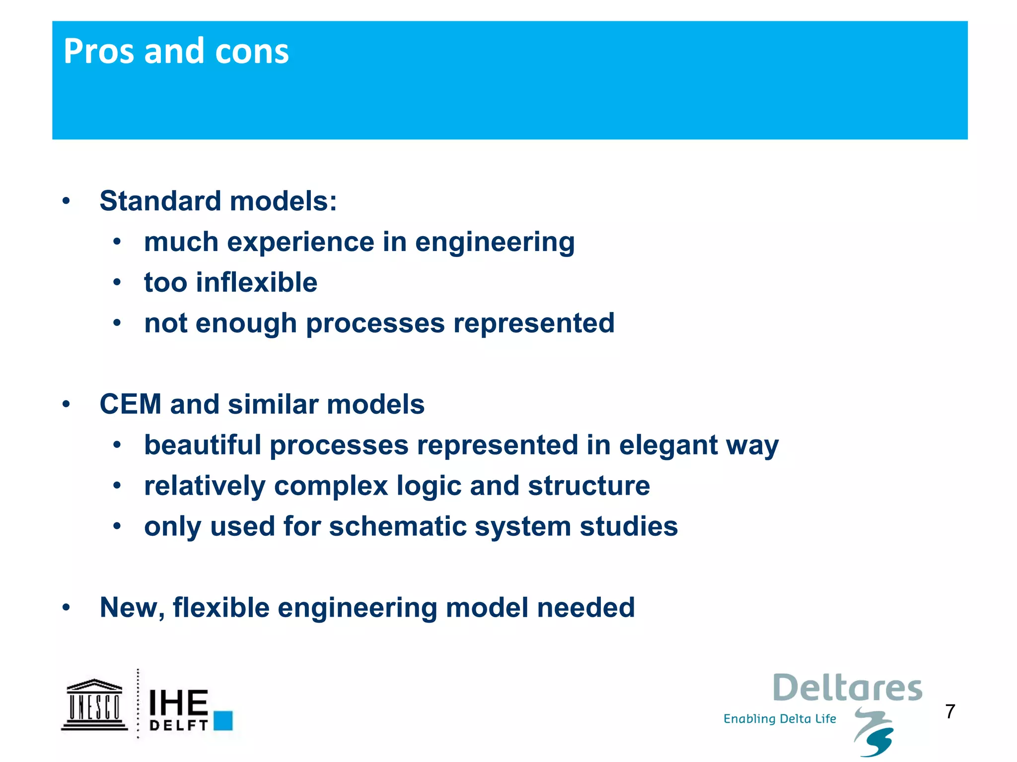
• Simple transport
formulas
• Based on deep water
wave conditions or
conditions at breaker
line
• Similar behaviour as
function of deep water
wave angle
Transport formulations
Author Notation Formula
USACE, 1984
(simplified)
CERC1 5/2
0 sin 2( )s S locQ bH =
Ashton &
Murray, 2006
CERC2 12 1 6
5 5 5
2 0 cos ( )sin( )s S loc locQ K H T =
USACE, 1984 CERC3 5/2
1 sin2( )s sb locbQ b H =
Kamphuis,
1992
KAMP 2 1.5 0.75 0.25 0.6
502.33 sin (2 )s sb b locbQ H T m D −
=
Where:
b : calibration coefficient CERC1
1
/
, ~ 0.1 0.2
16( )(1 )s
k g k
b k
p
= −
− −
( )
sin( )
arctan 2
cos( )
j
j c w
loc i
c w i
−
=
−
1
5
2 1( )
2
g
K K
= , 1/2
1 0.4 /K m s
0sH : offshore significant wave height
sbH : significant breaking wave height
T : peak wave period
50D : median grain diameter [m]
bm : mean bed slope (beach slope in the breaking zone)
b : breaking wave angle
Author Notation Formula
USACE, 1984
(simplified)
CERC1 5/2
0 sin 2( )s S locQ bH =
Ashton &
Murray, 2006
CERC2 12 1 6
5 5 5
2 0 cos ( )sin( )s S loc locQ K H T =
USACE, 1984 CERC3 5/2
1 sin2( )s sb locbQ b H =
Kamphuis,
1992
KAMP 2 1.5 0.75 0.25 0.6
502.33 sin (2 )s sb b locbQ H T m D −
=
Where:
b : calibration coefficient CERC1
1
/
, ~ 0.1 0.2
16( )(1 )
k g k
b k
p
= −
− −
Transport is a function of wave
height and wave direction
Maximum at around 45o relative to
coast](https://image.slidesharecdn.com/dsd-int2019shorelinesandfuturecoastlinemodelling-roelvink-191218115943/75/DSD-INT-2019-ShorelineS-and-future-coastline-modelling-Roelvink-12-2048.jpg)
![13
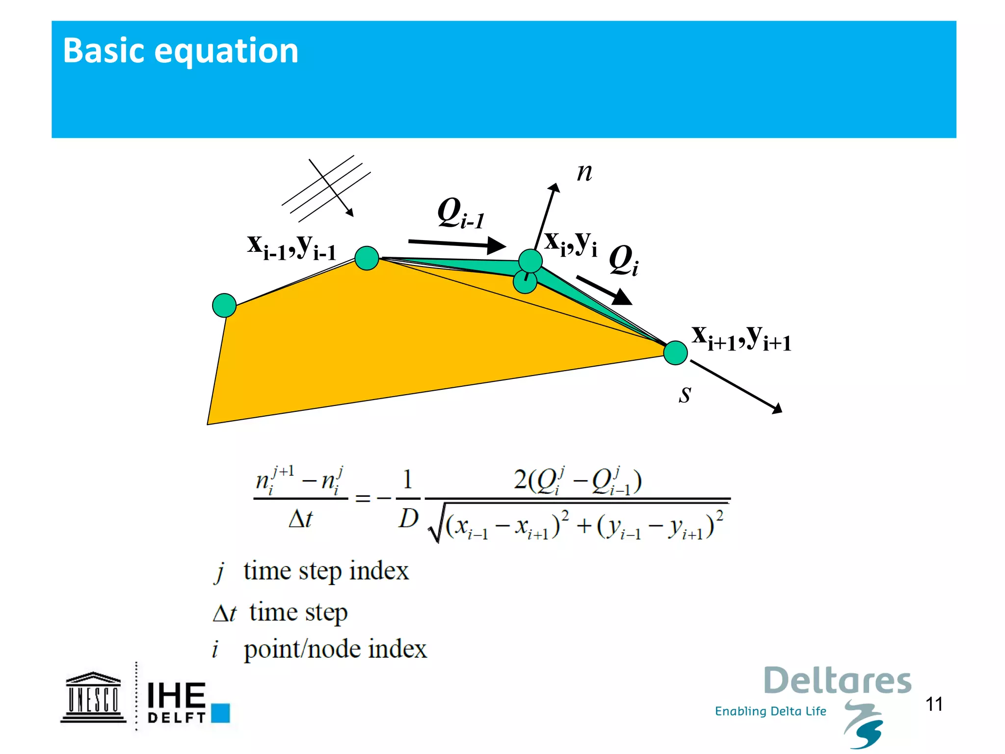
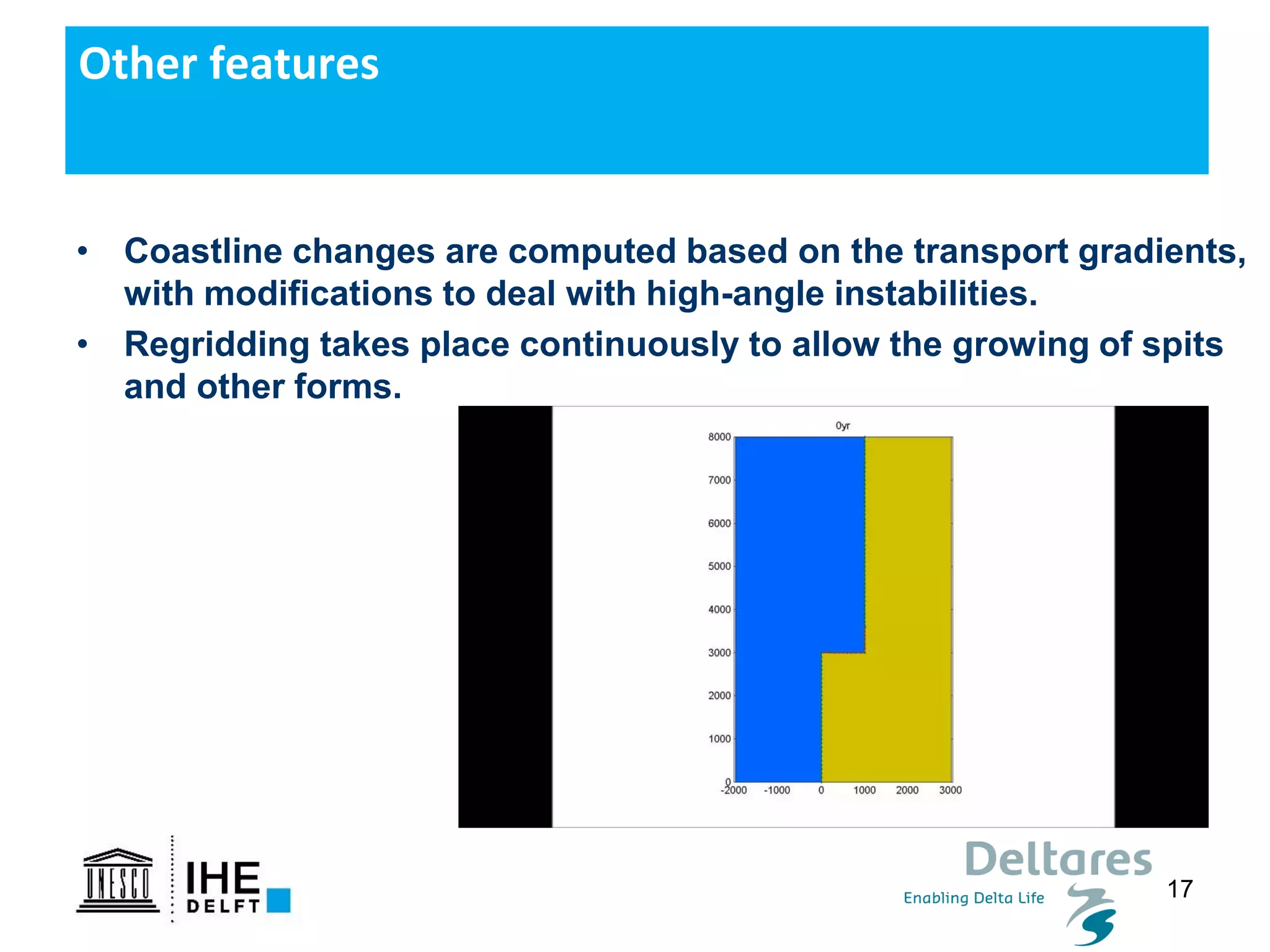
Representation of coastline and structures
• Coastline is represented as an arbitrary number of free-form
polylines that can be open or closed (islands)
0 2000 4000 6000 8000 10000
0
1000
2000
3000
4000
5000
6000
7000
8000
9000
10000
Easting [m]
Northing[m]
Add coastline (LMB); Next segment (RMB); Exit (q)
0 2000 4000 6000 8000 10000
0
1000
2000
3000
4000
5000
6000
7000
8000
9000
10000
Easting [m]
Northing[m]
Add structure (LMB); Next structure (RMB); Exit (q)](https://image.slidesharecdn.com/dsd-int2019shorelinesandfuturecoastlinemodelling-roelvink-191218115943/75/DSD-INT-2019-ShorelineS-and-future-coastline-modelling-Roelvink-13-2048.jpg)
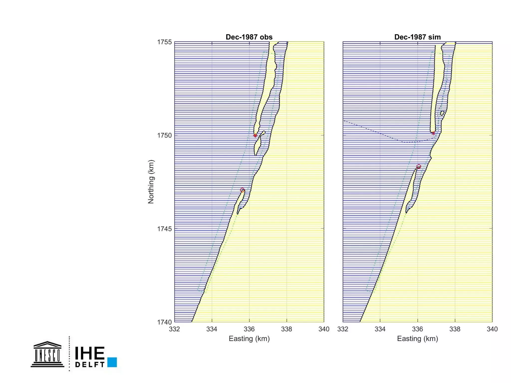


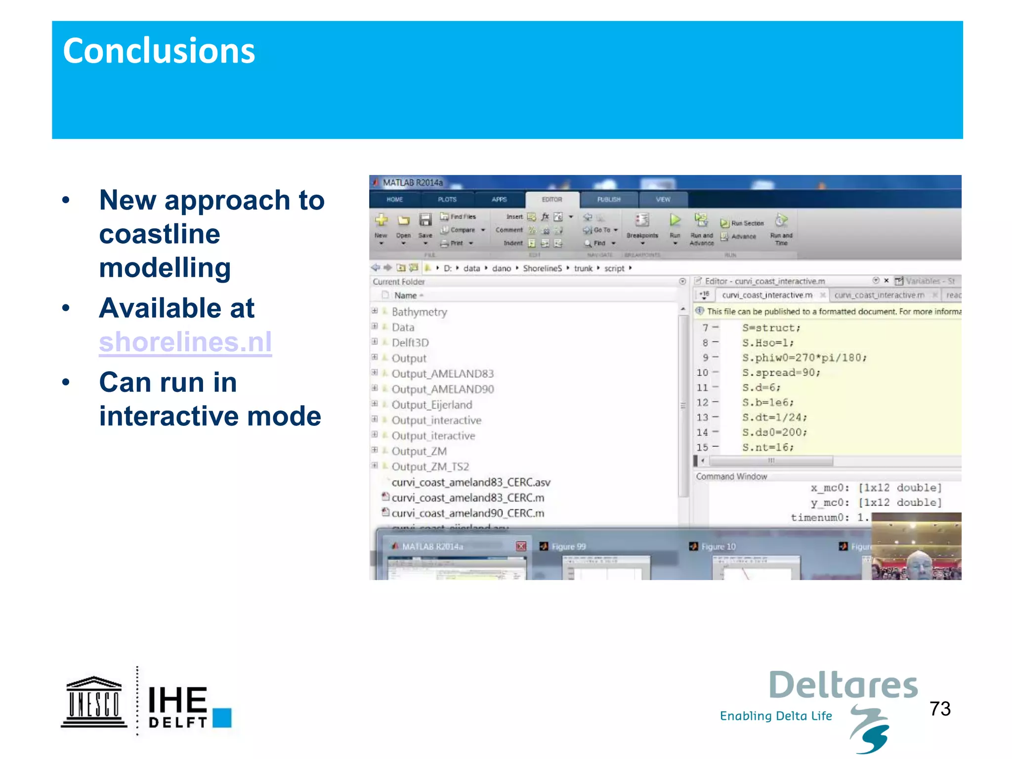

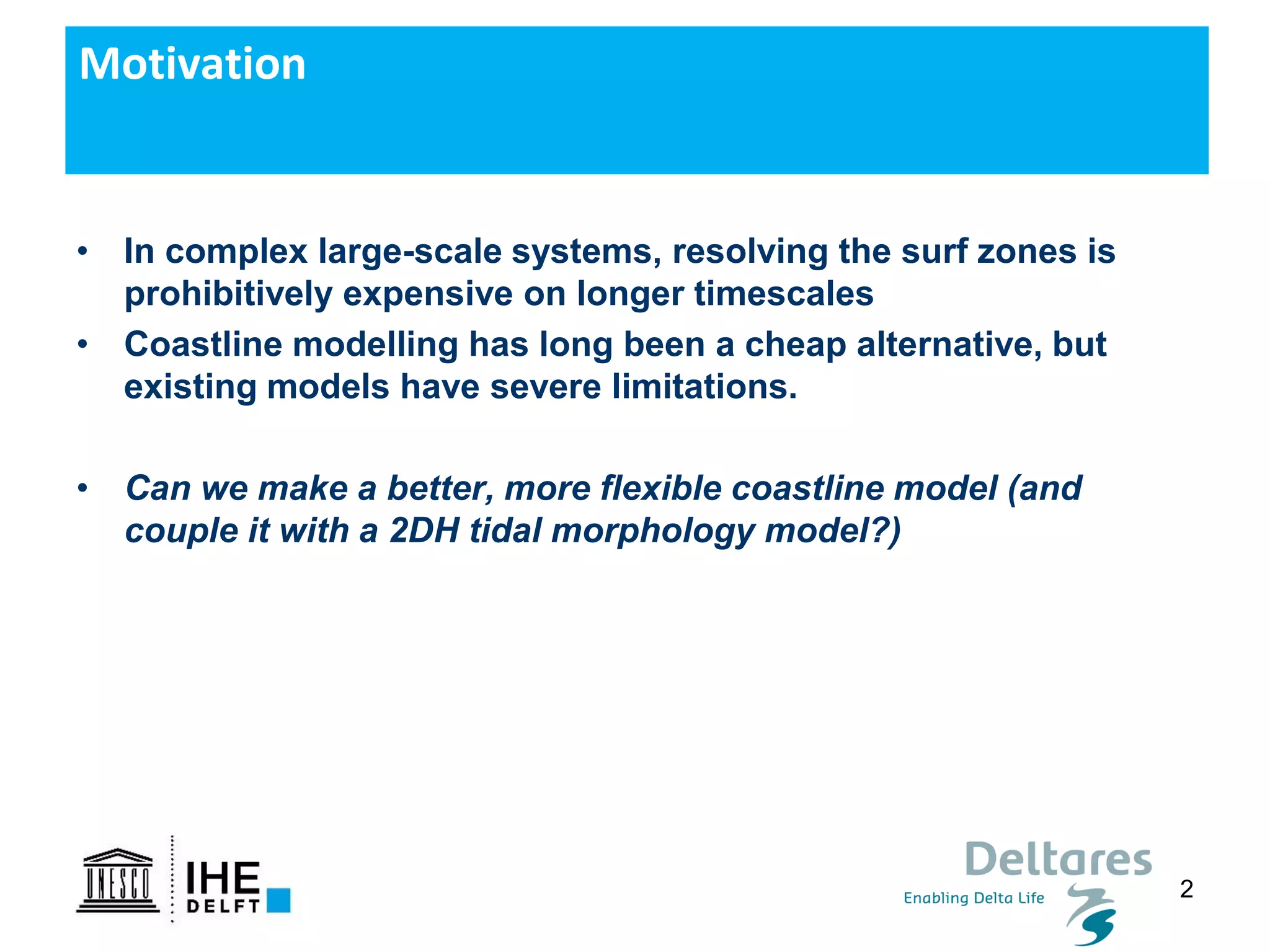
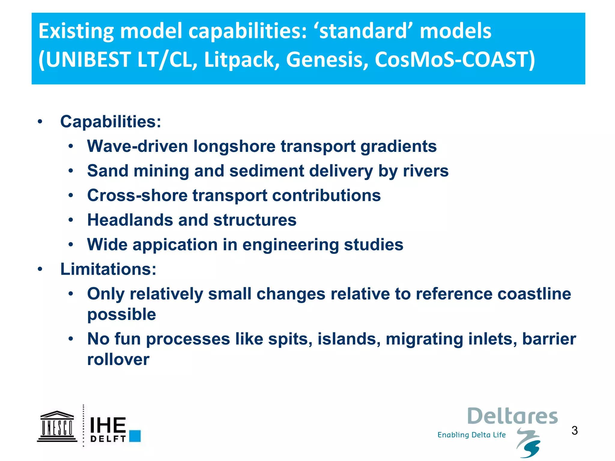
The document discusses the development of a new, more flexible coastline modeling approach to overcome limitations of current models, which are inflexible and inadequate in representing dynamic coastal processes. This new prototype model can effectively simulate complex coastal phenomena, requires minimal input, and is available as open-source MATLAB code. The authors aim to improve accuracy in engineering studies of coastlines while facilitating the integration of additional processes.