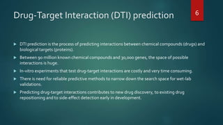
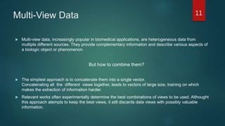
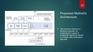
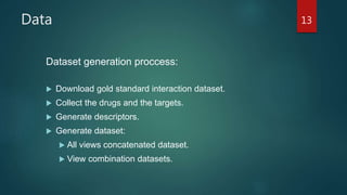
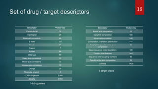
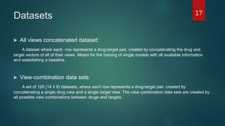
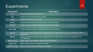
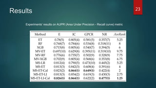
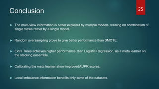
- The document proposes a multi-view stacking ensemble method for drug-target interaction (DTI) prediction that combines predictions from multiple machine learning models trained on different drug and target feature view combinations. - It generates 126 view combination datasets from 14 drug views and 9 target views, then trains extra trees, random forest, and XGBoost classifiers on each view combination. Predictions from these base models are then combined using a stacking ensemble with an extra trees meta-learner. 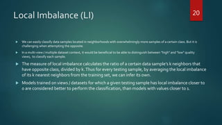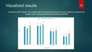- The method is shown to outperform single models and voting ensembles, and calibration of the meta-learner and use of local imbalance measures provide further improvements to predictive performance on DTI prediction tasks.

1. Multi-View DTI
Prediction
DIMITRIS PAPADOPOULOS, AEM 41
MSc DATA ANDWEB SCIENCE
DEPARTMENT OF INFORMATICS, AUTH
SUPERVISOR: PROF. GRIGORIOS
TSOUMAKAS
1

2. Contents
Introduction
Method taxonomy
Data
Proposed method
Experiments
Future research
2

3. Introduction
Method taxonomy
Data
Proposed method
Experiments
Future research
3

4. Introduction
 Drug discovery is the process of finding a chemical
compound that interacts (binds) with a certain biological
target (protein), mimicking or blocking its physiological
function, so that it acts therapeuticly on a disease.
But …
 Costs around 1.8 billion $
 Takes more than 10 years
 Failure rate is more than 90%
4

5. Drug Discovery Timeline
Target
discovery
2 - 3 years
Hits discovery
0.5 – 1 year
Lead selection
and optimization
1 – 3 years
ADMET
1 – 2 years
Clinical trials
5 – 6 years
Registration
1 – 2 years
DTI prediction
5

6. Drug-Target Interaction (DTI) prediction
 DTI prediction is the process of predicting interactions between chemical compounds (drugs) and
biological targets (proteins).
 Between 90 million known chemical compounds and 30,000 genes, the space of possible
interactions is huge.
 In-vitro experiments that test drug-target interactions are costly and very time consuming.
 There is need for reliable predictive methods to narrow down the search space for wet-lab
validations.
 Predicting drug-target interactions contributes to new drug discovery, to existing drug
repositioning and to side-effect detection early in development.
6

7. Introduction
Method taxonomy
Data
Proposed method
Experiments
Future research
7

8. Method taxonomy
 Ligand-based:
• Predict interactions using similarities between protein ligands.
• Low performance
 Docking-based:
• Predict interactions using 3D structures of drug-target pairs to run simulations.
• Can not be applied when the protein’s 3D structure is unknown.
• Computationally costly
 Chemogenomic:
• Predict interactions using both drug and target information and are able to exploit
multi-view biological data.
• Versatile
• Can achieve SOTA performance.
8

9. Chemogenomic Approaches
 Neighborhood models:
Make use of a given drug or target closest neighboor’s interaction information.
 Bipartite models:
Use graph edge-prediction, predicting interactions based on drugs, then based on targets and finally
combine the predictions.
 Network diffusion models:
Make use of bipartite drug-target graphs and apply network diffusion algorithms.
 Matrix factorization models:
Apply matrix factorization techniques, inspired from recommender systems.
 Feature-based models:
Represent drugs and targets with descriptive vectors, which are used as features to train machine
learning models.
9

10. Feature-based Methods' Problem
Formulation
 Binary Classification:
Most commonly the DTI problem is formulated as a binary classification task, where between drug and
target pairs the interactivity (0 or 1) accounts for the class and the concatenated drug-target descriptor
vectors accounts for the sample features.
 Multiclass - Multilabel Classification:
In the multiclass - multilabel formulation of the problem, only the drugs' or the targets' vectors are used,
in order to train a model to predict interacting drugs or targets as labels.
 Regression:
As the drugs efficacy is dose related, it is reasonable to approach the problem as a regression task,
where the data used are drug-target vectors (as in binary classification), but the predicted value is a
continuous number, representing the intensity of the interaction.
10

11. Multi-View Data
 Multi-view data, increasingly popular in biomedical applications, are heterogeneous data from
multiple different sources. They provide complementary information and describe various aspects of
a biologic object or phenomenon.
But how to combine them?
 The simplest approach is to concatenate them into a single vector.
Concatenating all the different views together, leads to vectors of large size, training on which
makes the extraction of information harder.
 Relevant works often experimentally determine the best combinations of views to be used. Althought
this approach atempts to keep the best views, it still discards data views with possibly valuable
information.
11

12. Introduction
Method taxonomy
Data
Proposed method
Experiments
Future research
12

13. Data
Dataset generation proccess:
 Download gold standard interaction dataset.
 Collect the drugs and the targets.
 Generate descriptors.
 Generate dataset:
 All views concatenated dataset.
 View combination datasets.
13

14. Gold standard dataset for DTI prediction
Dataset Drugs Targets Drug – target pairs Interactions
Ε 445 664 295.480 2.926
ΙC 210 204 42.840 1.476
GPCR 223 95 21.185 635
NR 54 26 1.404 90
Yamanishi dataset1
14

15. Drug / Target Collection
 Drug collection:
Collect drugs SMILES representation from DrugBank and Kegg databases.
Simplified molecular-input line-entry system (SMILES) is a way to encode drug molecular structures
in the form of line notation, using short ASCII strings.
 Target collection:
Collect targets' amino acid sequences from Kegg database.
Each amino acid is represented with a letter of the English alphabet and a specific combination of
them, forms a sequence that includes the information of the protein’s structure.
15

16. Set of drug / target descriptors
Descriptor Vector size
Constitutional 30
Topological 25
Molecular connectivity 44
E-state 237
Basak 21
Kappa 7
Burden 64
MOE-type 60
Geary auto-correlations 32
Moran auto-correlations 32
Moreau auto-correlations 32
Charge 25
Molecular property 6
ECFP4 fingerprint 2.048
Σύνολο 2.663
Descriptor Vector size
Amino acid composition 20
Dipeptide composition 400
Moran autocorrelation 240
Composition, Transition, Distribution 147
Amphiphilic pseudo amino acid
composition
80
Quasi-sequence order descriptors 100
Conjoint triad features 343
Sequence order coupling numbers 60
Pseudo amino acid composition 30
Σύνολο 1.420
9 target views
14 drug views
16

17. Datasets
 All views concatenated dataset:
A dataset where each row represents a drug-target pair, created by concatenating the drug and
target vectors of all of their views. Meant for the training of single models with all available information
and establishing a baseline.
 View-combination data sets:
A set of 126 (14 Χ 9) datasets, where each row represents a drug-target pair, created by
concatenating a single drug view and a single target view. The view combination data sets are created by
all possible view combinations between drugs and targets.
17

18. Introduction
Method taxonomy
Data
Proposed method
Experiments
Future research
18

19. Proposed Method's
Architecture
 The proposed method is a
Stacking ensemble, for
combining the outputs of
multiple ML algorithms trained
on multiple view-combination
data sets.
19

20. Local Imbalance (LI)
 We can easily classify data samples located in neighborhoods with overwhelmingly more samples of a certain class. But it is
challenging when attempting the opposite.
 In a multi-view / multiple dataset context, it would be beneficial to be able to distinguish between "high" and "low" quality
views, to classify each sample.
 The measure of local imbalance calculates the ratio of a certain data sample’s k neighbors that
have opposite class, divided by k.Thus for every testing sample, by averaging the local imbalance
of its k nearest neighbors from the training set, we can infer its own.
 Models trained on views / datasets for which a given testing sample has local imbalance closer to
0 are considered better to perform the classification, than models with values closer to 1.
20

21. Introduction
Method taxonomy
Data
Proposed method
Experiments
Future research
21

22. Experiments
Experiment Description
ET Extra Trees model trained on all views
RF Random Forest model trained on all views
XGB XGBoost model trained on all views
MV-ET Voting ensemble consisting of ETs trained on view combinations
MV-RF Voting ensemble consisting of RFs trained on view combinations
MV-XGB Voting ensemble consisting of XGBs trained on view combinations
MS-LR Stacking ensemble consisting of the 3 algorithms (ΕΤ, RF, XGB) trained on all view combinations, with LR
meta-learner
MS-ET Stacking ensemble consisting of the 3 algorithms (ΕΤ, RF, XGB) trained on all view combinations, with
ET meta-learner
MS-ET-Cal MS-ET model, with probability calibration of the meta-learner
MS-ET-LI MS-ET model, with local imbalance information
MS-ET-LI-Cal MS-ET-Cal model, with local imbalance information
22

23. Results
Experiments' results on AUPR (Area Under Precision - Recall curve) metric
23

24. Visualized results
Visualized AUPR results of the models with the best performance from each category of experiments
(single model, voting ensemble and stacking ensemble)
24

25. Conclusion
 The multi-view information is better exploited by multiple models, training on combination of
single views rather by a single model.
 Random oversampling prove to give better performance than SMOTE.
 Extra Trees achieves higher performance, than Logistic Regression, as a meta learner on
the stacking ensemble.
 Calibrating the meta learner show improved AUPR scores.
 Local imbalance information benefits only some of the datasets.
25

26. Introduction
Method taxonomy
Data
Proposed method
Experiments
Future research
26

27. Future Work
 Asses proposed method’s predictive performance on
scenarios S2,S3,S4.
 Experiment applying dimensionality reduction.
 Add more data views for the description of drugs and
targets.
 Add 2 by 2 views combination datasets
 Apply ensemble pruning techniques to decrease the
number of participating models.
 Experiment trainning the meta learner along with the
predictions of the base learners, also with the
samples' vectors.
27

28. Thank you for your attention
28