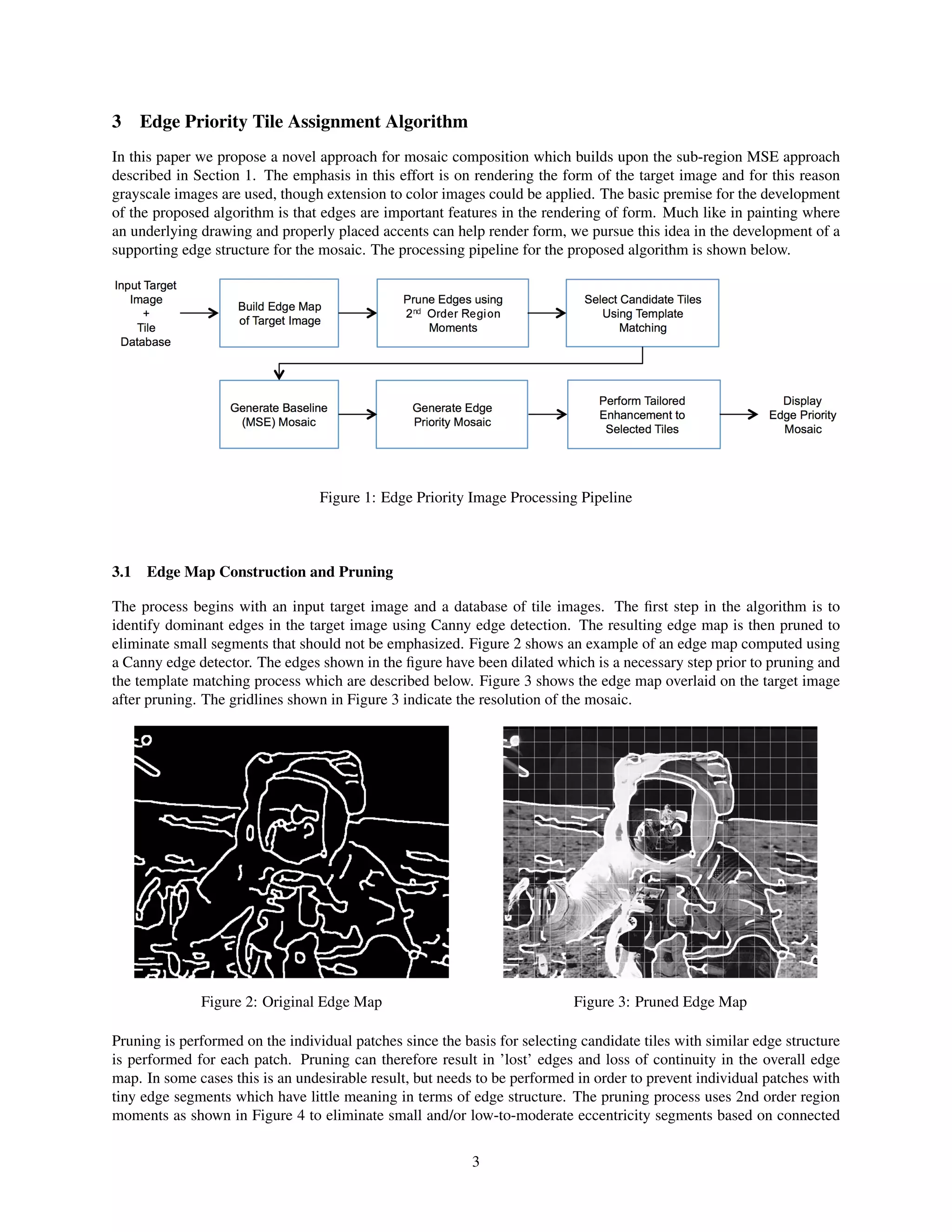
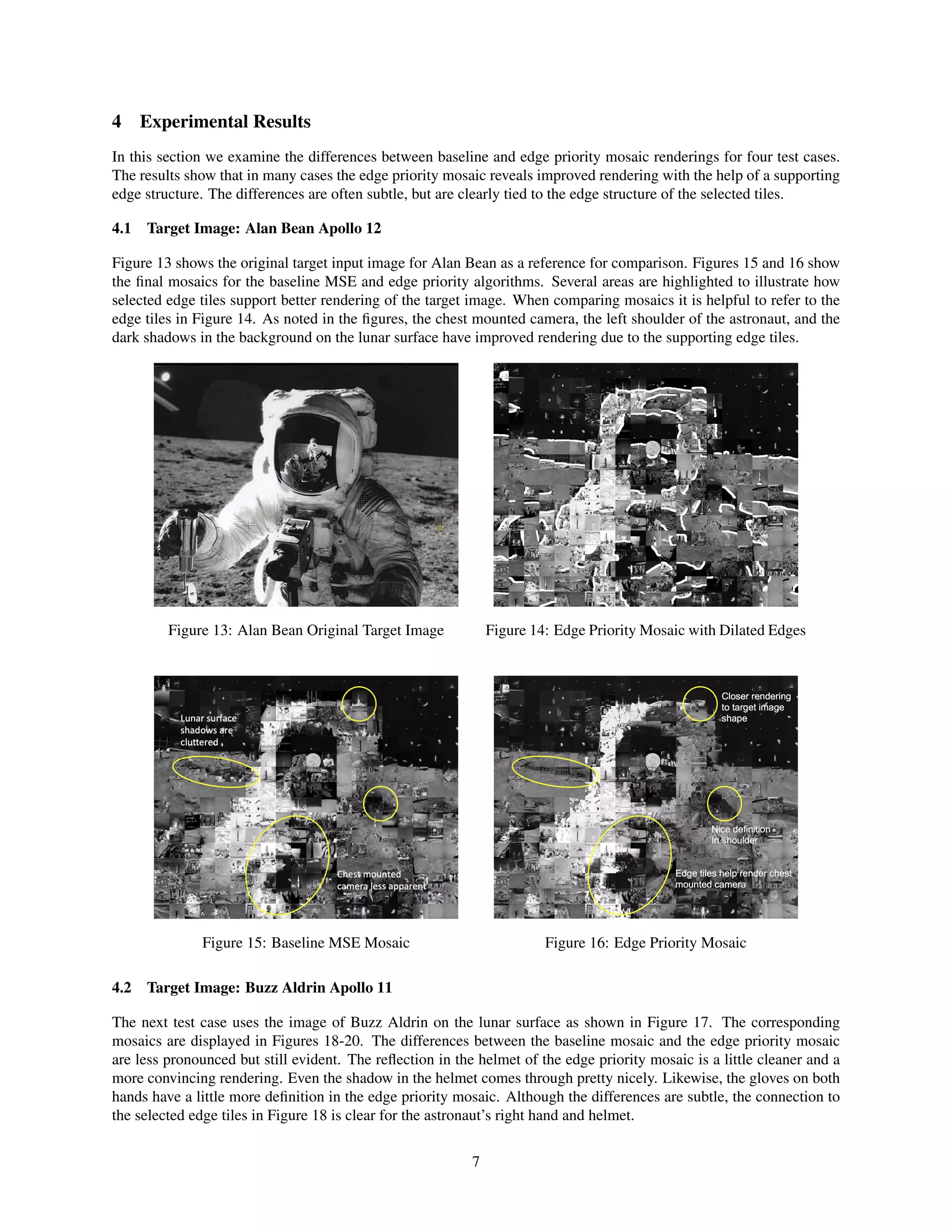
This document proposes a novel algorithm for composing digital mosaics using edge priority tile assignment. It begins by detecting edges in the target image and pruning small edges. Candidate tiles with similar edge structures are identified through template matching. A baseline mosaic is generated using mean square error criteria for tile assignment. Then, a second pass assigns tiles to edge regions, preferring candidate edge tiles if their MSE is within a threshold of the baseline. Optionally, edge tiles can be enhanced to further draw out the target image form. Experimental results on Apollo mission photos show the edge priority mosaic better reveals form through a supporting edge structure.

1. Digital Composition of Mosaics using Edge Priority Tile Assignment
William Kromydas
bkromydas@gmail.com
Department of Electrical Engineering
Stanford University
Abstract
Composition of mosaics from smaller tile images has a long history and many interesting appli-
cations. In the digital age, the opportunities for composing mosaics from many thousands of tile
images is achieved through automation. Incorporation of thematic content in mosaics adds an ap-
pealing dimension with applications in art, history, education, advertising, and marketing. In this
paper, we explore the use of image processing techniques for automated digital composition of
mosaics using a relatively small database of tile images with thematic content related to the target
image. Existing techniques based on sub-region analysis and mean square error (MSE) criteria for
tile assignment are leveraged for composition of a baseline mosaic. In order to meet the challenge of
limited datasets, a novel algorithm is proposed that identifies dominant edges in the target image as a
basis for a 2nd tier tile assignment process that results in an ’edge priority’ mosaic. An optional step
is also proposed in which the edge priority mosaic can be further enhanced based on the edge struc-
ture in the target image. The final stage enhancement process opens the possibility to further draw
out the form and likeness of the subject matter in the target image and also offer an opportunity for
incorporating artistic effects in the final rendering. Experimental results show improved rendering
with modest size tile databases over baseline MSE mosaics produced using sub-region techniques.
1 Introduction
Numerous and creative techniques have been developed over the years in the generation of mosaics. One of the earliest
examples of the concept is the abstract painting of Abraham Lincoln by Salvador Dali. In the early 1980s, K. Knowlton
patented a technique that used dominos exclusively as the tiling element. In 1990, Haeberli [1] developed a method
that used a painted brush stroke as the tiling element to achieve a ”painterly” quality in the final image. Inspired by
Knowtton’s work, Rob Silvers began developing computer generated mosaics in the 1990s. The methods he developed
reach a high level of sophistication in digital composition in which his mosaics reveal an underlying story through the
deliberate selection of tiles that embody a theme related to the target image. As noted in his book [2], blue skies
are filled with birds and planes, water with fish; faces were made from people. His use of sub-region analysis and
tile composition is highly effective with superb rendering of form, value, texture and color harmony all unified with
underlying and connected themes.
1

2. The objective for this effort is to explore the development of an algorithm that meets the challenges of limited datasets
which is relatively common for theme-based images. We also strive to develop mosaics where the tile images represent
a significant component in the final rendering of the target image. This allows for a content-rich representation and also
presents a formidable challenge for rendering due to the relative low number of tiles in the mosaic. For any viewing
scale the number of tile images in the mosaic is assumed to be no more than 300-500 hundred. For example, a 16” x
20” mosaic with 320 tiles would contain 1” square tiles. A proper composition would effectively increase the apparent
resolution of the final image while maintaining visual integrity of individual tiles. As a point of reference, some of the
mosaics created by Robert Silvers’ company, Runaway Technology can contain as many as 10,000 individual tiles.
The generation of mosaics can be quite sophisticated, however, the general process is outlined in many references and
typically includes the steps below at various levels of sophistication.
• Acquisition of a large database of images to work with that contain adequate variation in color, shape, value
and texture (and possibly semantic content)
• A target image to serve as the model
• A grid-based system for both the target image and tiles for discrete modeling and region characterization
• One or more feature descriptors that will be used in the tile selection process
• Formation of an aggregate feature vector
• Evaluation of a similarity measure for making tile assignments
There are numerous approaches for implementing feature extraction, but many algorithms make use of sub-region
analysis which begins with partitioning the target image into patches. Each patch is then subdivided into a sub-region
grid. Similarly, each tile image is also sub-divided into sub-regions at the same resolution as the target patches. Image
features are then extracted from target patches and database tiles and a similarity measure (e.g. L-1 or L-2 distance)
is computed between a given target image patch and a tile. The tile with lowest distance score is selected as the tile
in the mosaic for the corresponding target image patch. References [3] and [4] are good sources for more in-depth
discussion in this area. Depending on the resolution of the sub-region grid and number of tiles available to select from,
this algorithm can produce some very satisfying results. The approach taken in [3] is more sophisticated than presented
here, but the underlying concept is similar. In this paper the above algorithm is implemented and the corresponding
mosaic is referred to as the baseline MSE mosaic. This will serve as a useful basis for comparison and is incorporated
as a first stage processing function in the approach outlined in this paper.
2 Data Acquisition and Preprocessing
Two datasets were acquired for use in this study: Eight thousand random flickr images [5] and 4,653 historical images
from the Apollo Lunar Program from five different missions [6] which were derived from [7]. Experimentation was
performed on the flickr images during initial code development. The main focus in this work is on thematic content
with limited datasets and the Apollo dataset served this purpose well. The Apollo data set contains images from all
mission phases including astronaut training, press photos, and events surrounding the missions. Many of the photos
from the actual missions contain numerous near duplicate images, so while a mosaic may appear to contain some
duplicates these are actually different images. The near repetition in the data set has pros and cons. In some sense the
effective size of the data set is much less than the total number of images due to many similar images. An alternate
viewpoint is that near duplicates might be advantageous if a particle structure is needed in multiple places within the
mosaic. It’s difficult to say if this data set is representative of a typical 4-5K size dataset but these observations are
mentioned because the percentage of near duplicate images is probably unusual.
A stand-alone pre-processing program was created to crop and resize the tile images. In order to keep the implemen-
tation straight forward, tile images were cropped in square proportion. Landscape images were center cropped and
portrait images were cropped at the top portion of the image as suggested by [3] to maximize the probability that the
cropped image contains the center of interest. Images were then resized to [50 x 50] pixels. Normalization of the
images was not performed in this implementation but should be investigated to determine what additional affect that
might have. In this application, tile images are the same size as patches in the target image and are selected based on
intensity value and edge structure similarity to the corresponding patch.
2

3. 3 Edge Priority Tile Assignment Algorithm
In this paper we propose a novel approach for mosaic composition which builds upon the sub-region MSE approach
described in Section 1. The emphasis in this effort is on rendering the form of the target image and for this reason
grayscale images are used, though extension to color images could be applied. The basic premise for the development
of the proposed algorithm is that edges are important features in the rendering of form. Much like in painting where
an underlying drawing and properly placed accents can help render form, we pursue this idea in the development of a
supporting edge structure for the mosaic. The processing pipeline for the proposed algorithm is shown below.
Figure 1: Edge Priority Image Processing Pipeline
3.1 Edge Map Construction and Pruning
The process begins with an input target image and a database of tile images. The first step in the algorithm is to
identify dominant edges in the target image using Canny edge detection. The resulting edge map is then pruned to
eliminate small segments that should not be emphasized. Figure 2 shows an example of an edge map computed using
a Canny edge detector. The edges shown in the figure have been dilated which is a necessary step prior to pruning and
the template matching process which are described below. Figure 3 shows the edge map overlaid on the target image
after pruning. The gridlines shown in Figure 3 indicate the resolution of the mosaic.
Figure 2: Original Edge Map Figure 3: Pruned Edge Map
Pruning is performed on the individual patches since the basis for selecting candidate tiles with similar edge structure
is performed for each patch. Pruning can therefore result in ’lost’ edges and loss of continuity in the overall edge
map. In some cases this is an undesirable result, but needs to be performed in order to prevent individual patches with
tiny edge segments which have little meaning in terms of edge structure. The pruning process uses 2nd order region
moments as shown in Figure 4 to eliminate small and/or low-to-moderate eccentricity segments based on connected
3

4. region eccentricity and region major-axis length (relative to the image patch size). Each connected region within a
patch is treated as an edge with configurable thresholds for the degree of pruning. In Figure 4, notional region ellipses
are displayed for those regions that were pruned due to eccentricity or major-axis length values. Figure 5 shows the
final edge map after pruning has been performed. The patches highlighted in yellow indicate the regions that were
pruned. Note that patches can contain multiple connected regions with each connected region treated as an edge.
If a patch contains multiple regions then the region with the longest major-axis length is considered in the pruning
process. As currently implemented, when multiple regions exist within a patch the entire patch is pruned or it is not
(based on the longest region in the patch). This can result in patches that survive the pruning stage, yet contain small
insignificant segments. In addition to region moments, other constraints are also utilized during pruning. For example,
the percentage of foreground to background is computed for each patch and if that ratio exceeds a certain threshold the
entire patch is pruned from the edge map. There is also a configurable threshold for the maximum number of regions
that may be contained in a patch and survive the pruning process. To summarize, it is the patch that is pruned (or not)
based on the pruning criteria applied to the longest region (edge) in the patch.
Figure 4: Region Moments Figure 5: Pruned Edge Map
3.2 Selecting Candidate Edge Tiles
After edge pruning has been performed the next step in the algorithm is to identify all tile images in the database which
have a similar edge structure to each patch in the target image that contains one or more edges. Similar to the target
image, an edge map is computed for each tile in the database using a Canny edge detector. The tiles typically require
a different set of Canny edge detector tuning parameters so that a single edge is produced as an edge map for the tile.
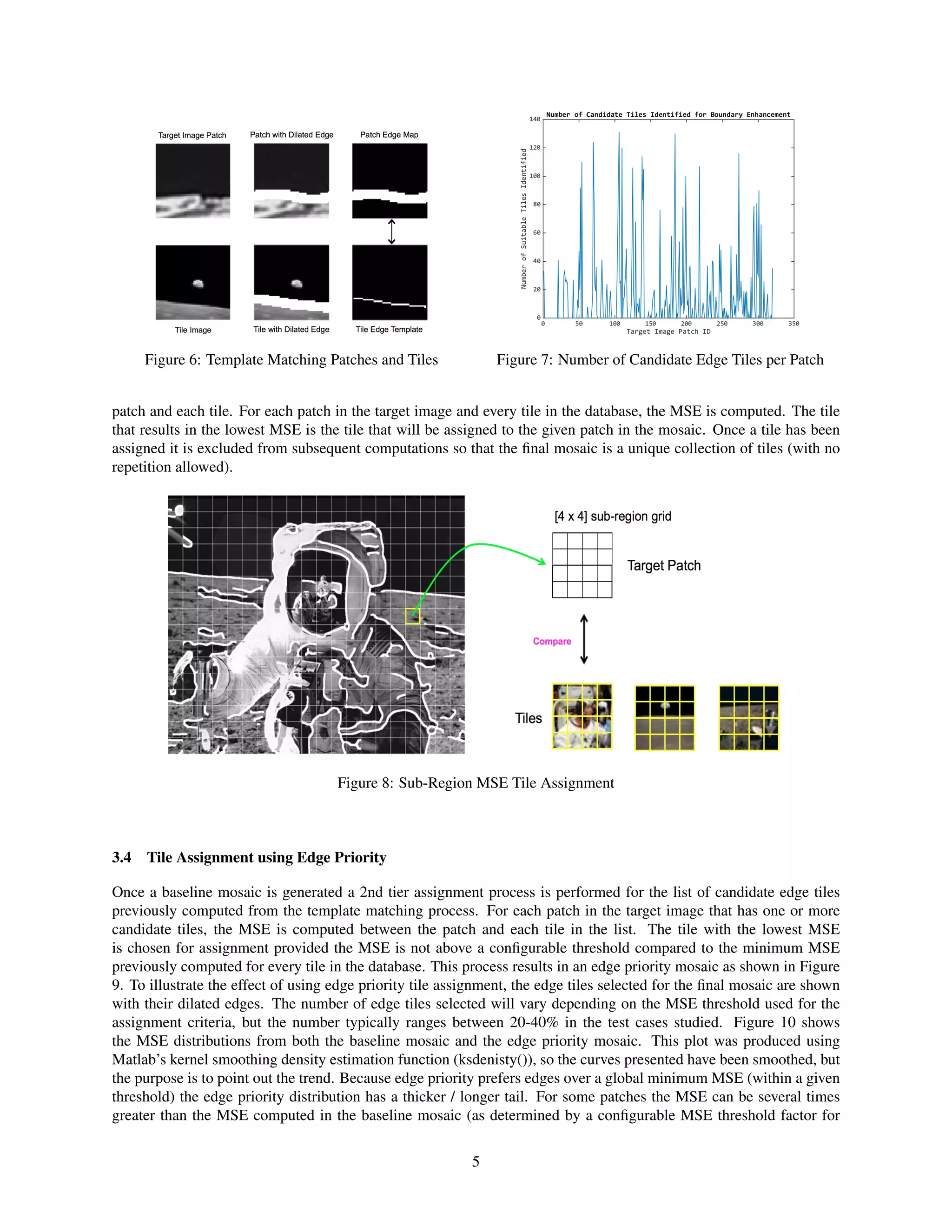
Selecting candidate tiles is accomplished by template matching where the single, pixel-wide edge in each tile image
is compared to the dilated edges in the target patches. Figure 6 illustrates the process in which template matching is
performed between each tile in the database and a dilated edge in a given patch. The amount of dilation in the image
patch is a configurable parameter which controls the goodness of fit required. There is also a configurable parameter
that requires the tile edge to be a certain percentage (region length) of the corresponding (dilated) edge in the patch.
The template matching process results in a list of one or more candidate ’edge’ tiles for each patch in the target image
that contains an edge. The diagnostic plot shown in Figure 7 was produced from the pruned edge map shown in Figure
3. In the current implementation, no consideration is given to the gradient of the edges at this stage in the algorithm.
This may therefore result in some template matches where a tile and the corresponding patch have opposing gradients,
however, such ’matches’ would be filtered out in downstream processing when the MSE test is made for final tile
assignment. A future implementation should consider checking the gradient in both images prior to declaring a match.
3.3 Generating a Baseline Mosaic
The previous sections set the stage for edge priority assignment, and now the process begins for composing a baseline
mosaic using sub-region analysis with a MSE criteria for tile assignment. Figure 8 illustrates the process in which
each target image patch and each tile in the database are sub-divided into a [4 x 4] sub-region grid. For each grid cell
in the sub-divided grid, the average grayscale intensity is computed and a 16-length feature vector is formed for each
4

5. Figure 6: Template Matching Patches and Tiles Figure 7: Number of Candidate Edge Tiles per Patch
patch and each tile. For each patch in the target image and every tile in the database, the MSE is computed. The tile
that results in the lowest MSE is the tile that will be assigned to the given patch in the mosaic. Once a tile has been
assigned it is excluded from subsequent computations so that the final mosaic is a unique collection of tiles (with no
repetition allowed).
Figure 8: Sub-Region MSE Tile Assignment
3.4 Tile Assignment using Edge Priority
Once a baseline mosaic is generated a 2nd tier assignment process is performed for the list of candidate edge tiles
previously computed from the template matching process. For each patch in the target image that has one or more
candidate tiles, the MSE is computed between the patch and each tile in the list. The tile with the lowest MSE
is chosen for assignment provided the MSE is not above a configurable threshold compared to the minimum MSE
previously computed for every tile in the database. This process results in an edge priority mosaic as shown in Figure
9. To illustrate the effect of using edge priority tile assignment, the edge tiles selected for the final mosaic are shown
with their dilated edges. The number of edge tiles selected will vary depending on the MSE threshold used for the
assignment criteria, but the number typically ranges between 20-40% in the test cases studied. Figure 10 shows
the MSE distributions from both the baseline mosaic and the edge priority mosaic. This plot was produced using
Matlab’s kernel smoothing density estimation function (ksdenisty()), so the curves presented have been smoothed, but
the purpose is to point out the trend. Because edge priority prefers edges over a global minimum MSE (within a given
threshold) the edge priority distribution has a thicker / longer tail. For some patches the MSE can be several times
greater than the MSE computed in the baseline mosaic (as determined by a configurable MSE threshold factor for
5

6. accepting edge tiles). Based on visual inspection of the final mosaics it is apparent that tiles with dominant edges can
perform well in the mosaic to help render certain shapes even though the MSE of a given tile might be significantly
higher than the one selected through a MSE criteria alone. In the cases studied this threshold ranged between 5 and 10,
though selected tiles did not necessary reach those limits. As this threshold is increased it becomes apparent that the
overall mosaic begins to break down with too much emphasis on edges and not enough on intensity matching within
a patch.
Figure 9: Edge Priority Mosaic Figure 10: Baseline and Edge Priority MSE
3.5 Tailored Tile Enhancement
The final step in the algorithm is optional. It involves tile image enhancement to draw out the form and likeness of
the target image. The basic idea is to use the original edge map as an indicator for which tiles to adjust. In order to
further emphasize the boundary indicated by the edge map, the remaining tiles can also be adjusted to subdue their
affect in rendering. The final rendering is shown in Figure 12 in which edge tiles were histogram adjusted to match
the histogram of the corresponding patch in the target image. All other tiles were contrast adjusted with a gamma of
0.9 to subdue their effect in the final mosaic. The type and magnitude of the enhancement can of course vary, but the
main idea presented is that the edge map is used as the indicator for tailored enhancements. The mosaic shown in
Figure 12 was composed using 4,653 images from the Apollo archive photo gallery [6,7].
Figure 11: Edge Priority Mosaic with Edge Map Overlay Figure 12: Final Rendering of Target Image
6

7. 4 Experimental Results
In this section we examine the differences between baseline and edge priority mosaic renderings for four test cases.
The results show that in many cases the edge priority mosaic reveals improved rendering with the help of a supporting
edge structure. The differences are often subtle, but are clearly tied to the edge structure of the selected tiles.
4.1 Target Image: Alan Bean Apollo 12
Figure 13 shows the original target input image for Alan Bean as a reference for comparison. Figures 15 and 16 show
the final mosaics for the baseline MSE and edge priority algorithms. Several areas are highlighted to illustrate how
selected edge tiles support better rendering of the target image. When comparing mosaics it is helpful to refer to the
edge tiles in Figure 14. As noted in the figures, the chest mounted camera, the left shoulder of the astronaut, and the
dark shadows in the background on the lunar surface have improved rendering due to the supporting edge tiles.
Figure 13: Alan Bean Original Target Image Figure 14: Edge Priority Mosaic with Dilated Edges
Figure 15: Baseline MSE Mosaic Figure 16: Edge Priority Mosaic
4.2 Target Image: Buzz Aldrin Apollo 11
The next test case uses the image of Buzz Aldrin on the lunar surface as shown in Figure 17. The corresponding
mosaics are displayed in Figures 18-20. The differences between the baseline mosaic and the edge priority mosaic
are less pronounced but still evident. The reflection in the helmet of the edge priority mosaic is a little cleaner and a
more convincing rendering. Even the shadow in the helmet comes through pretty nicely. Likewise, the gloves on both
hands have a little more definition in the edge priority mosaic. Although the differences are subtle, the connection to
the selected edge tiles in Figure 18 is clear for the astronaut’s right hand and helmet.
7

8. Figure 17: Original Target Image Figure 18: Edge Priority Tiles
Figure 19: Baseline MSE Mosaic Figure 20: Edge Priority Mosaic
4.3 Target Image: Gene Cernan Apollo 17
This next test case shows Gene Cernan standing next to the lunar rover. Figure 21 shows the original target image and
the same sequence as previously reported is shown in the remaining figures for comparison. Due to the smaller scale of
8

9. the forms in this image the mosaic resolution was increased to 480 tiles [20 x 24]. In spite of the increased resolution,
and as a point of reference, the visor on the astronaut’s helmet spans the area of approximately four tiles. So rendering
detail at that level will be quite limited as illustrated in the results below. Nonetheless, the image is recognizable in the
mosaics. The antenna on the lunar rover is extremely faint but the structure is evident. In this test case the mosaics are
quite comparable. The final stage enhancement to the edge-priority mosaic draws out the subject matter form a little
more, but of course such enhancements could also have been applied to the baseline mosaic. In terms of improved
rendering due to edges only, the mosaics are very similar. There is one exception worth noting that stands out. The
definition in the astronaut’s left hand is clearly evident due to the three edge tiles that surround the finger tips. This is
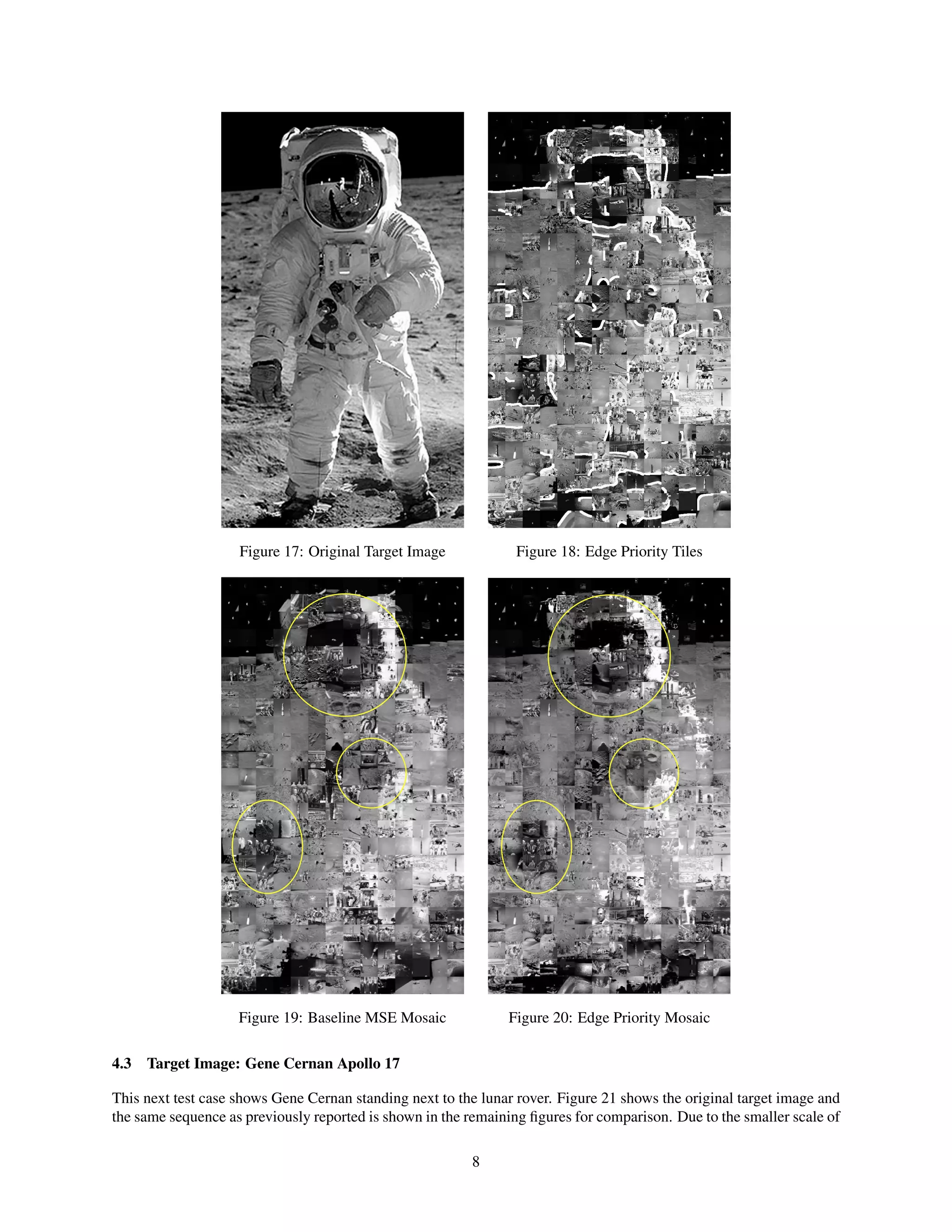
easily seen by comparing Figures 22 and 24.
Figure 21: Original Target Image Figure 22: Edge Priority Tiles
Figure 23: Baseline MSE Mosaic Figure 24: Edge Priority Mosaic
4.4 Target Image: Apollo 11 Saturn-V Launch
The photo in Figure 25 of the Apollo 11 Saturn-V launch has significant historic appeal, but there is very little recog-
nizable form to render. A majority of the image is uniform gray sky, smoke and plume from the rocket launch and a
crowd of on-lookers in the foreground. The body of water is sunlight and uniform. An attempt is made to compose
a mosaic from this image with a relatively coarse tile structure [18 x 16] with only 288 tiles. The edge maps for
this image are shown in Figures 26 and 27. The main focal point of the launch tower and rocket are preserved after
pruning. The edges in the foreground however were substantially pruned and contain very little structure. A successful
rendering of such an image with thematic content in the tiles could prove to be a captivating mosaic.
9

10. Figure 25: Apollo 11 Launch Figure 26: Edge Map Figure 27: Pruned Edge Map
Figures 28 through 30 show the final mosaics. Figure 29 shows the original edge map superimposed on the edge
priority mosaic prior to final stage enhancement. It is evident in Figures 28 and 30, that the rocket is more apparent in
the edge priority mosaic than in the baseline MSE mosaic in Figure 28.
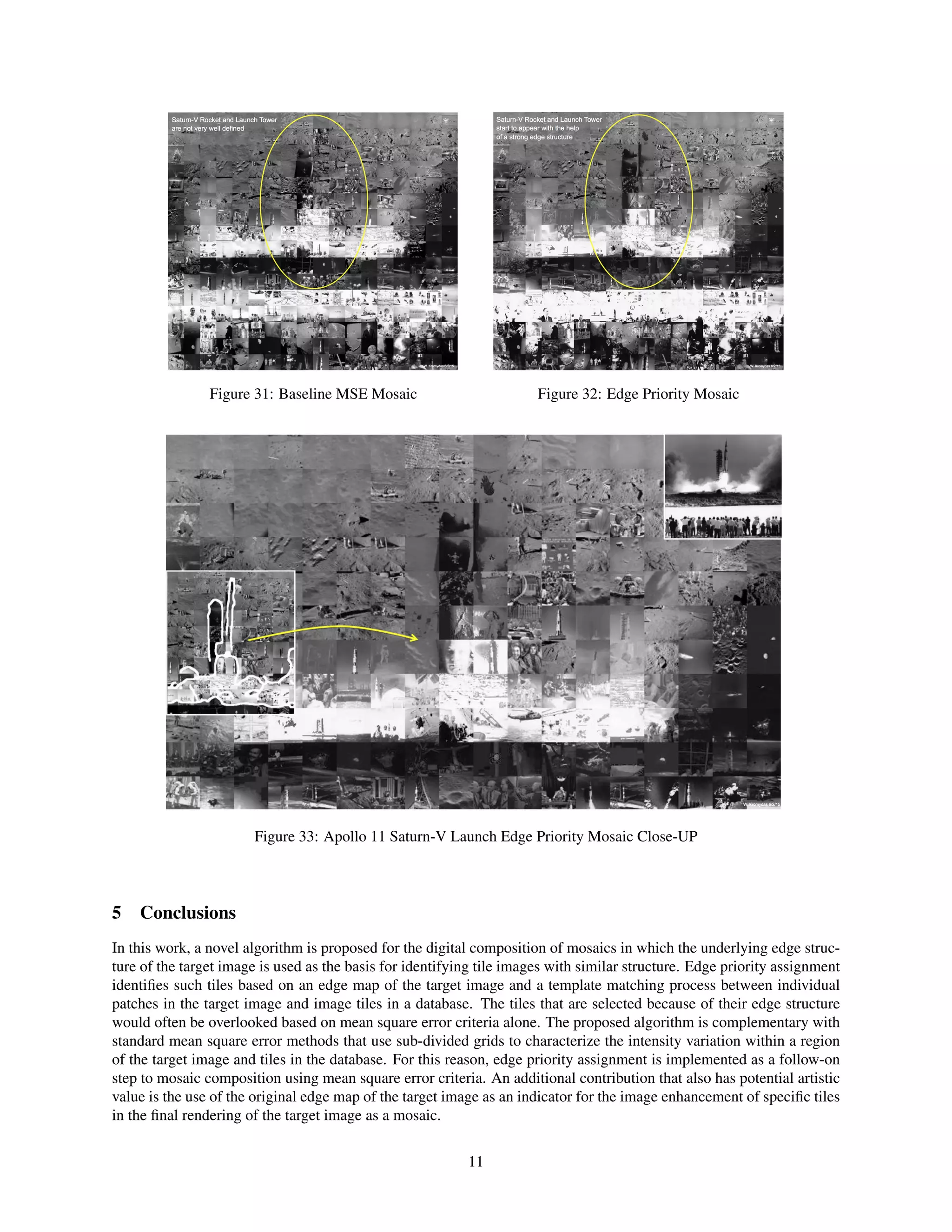
Figures 31 and 32 shows a direct comparison at a larger scale between the baseline MSE mosaic and the edge priority
mosaic which highlight the differences in how the launch tower and rocket are rendered in both images. The differences
are subtle and subjective, as this rendering is more abstract due to the nature and scale of the subject matter. Because
the rocket is narrow and only a single edge is used within a patch the rendered form only shows one side of the rocket.
Finally, Figure 33 offers a close-up view of the edge priority mosaic with an inset of the original image in the upper
right and another inset of the edge map to the left. What is most striking in this example is the strong thematic
rendering that occurs. The gray sky become a mosaic of the lunar surface and the dark smoke from the rocket plume
contains images from the blackness of space. The histogram matching that occurs for selected tiles is probably too
extreme, but the contrast adjustment of the remaining tiles has a nice effect. This is a prime example of the artistic
component that can be realized through the use of thematic images and image enhancement in the final rendering.
While this particular composition falls short in many respects, improved rendering of the crowd and the rocket may
be possible. An excursion test case was completed with an [8 x 8] sub-region grid which showed minor rendering
improvements but did achieve a leap in overall quality. The difficulty with this target image is the lack of form and
the scale of the objects in the image. A successful mosaic for such an image would be judged by whether the viewer
could appreciate it for what it is without knowledge of the source image content. A larger database of images to select
from might help, as well as algorithm tuning, but this test case also reveals the limitations of the current approach.
Continued study is required to determine how much this could be improved. Ideas for future work are presented in
Section 6 which were motivated by the test cases conducted in this study.
Figure 28: Baseline MSE Mosaic Figure 29: Edge Map Figure 30: Edge Priority Mosaic
10

11. Figure 31: Baseline MSE Mosaic Figure 32: Edge Priority Mosaic
Figure 33: Apollo 11 Saturn-V Launch Edge Priority Mosaic Close-UP
5 Conclusions
In this work, a novel algorithm is proposed for the digital composition of mosaics in which the underlying edge struc-
ture of the target image is used as the basis for identifying tile images with similar structure. Edge priority assignment
identifies such tiles based on an edge map of the target image and a template matching process between individual
patches in the target image and image tiles in a database. The tiles that are selected because of their edge structure
would often be overlooked based on mean square error criteria alone. The proposed algorithm is complementary with
standard mean square error methods that use sub-divided grids to characterize the intensity variation within a region
of the target image and tiles in the database. For this reason, edge priority assignment is implemented as a follow-on
step to mosaic composition using mean square error criteria. An additional contribution that also has potential artistic
value is the use of the original edge map of the target image as an indicator for the image enhancement of specific tiles
in the final rendering of the target image as a mosaic.
11

12. 6 Future Work
There are several areas that should be explored in further study. First, developing a proper edge map of the target
image that works well with the desired resolution of the mosaic is a significant challenge. Once the edge map for the
target image is cerated no further attention is given to neighboring patches in the current implementation. There may
be value in exploring a layered approach that considers continuity across the patch work, both in terms of creating
the final edge map and in the selection of tiles. The current approach is limited in the method used to determine the
similarity of the edge structure between a tile and a patch since it does not allow for more than one edge to be matched
between a patch and a tile. Finally, the use of final stage enhancement was only briefly experimented with. In order to
keep comparisons consistent across the test cases only a single setting was used. There are numerous possibilities and
strategies that could be explored using the edge map (or selected edge tiles) as an indicator for image adjustments.
7 Acknowledgements
I would like to thank Andr´e Filgueiras de Araujo for the discussions we had during the course of this project and for
his thoughtful comments and guidance.
This work is dedicated to the memory of Sebastian Capella (Spanish impressionist painter) who I was privileged to
have known and learned from.
8 Test Case MSE Plots
Figure 34: Alan Bean Figure 35: Buzz Aldrin
Figure 36: Gene Cernan Figure 37: Apollo 11 Launch
12

13. 9 Supplement
Figure 38: Alan Bean Self Portrait (painting) Figure 39: Edge Priority Mosaic
References
[1] P.E. Haeberli. Paint by Numbers: Abstract Image Representations, Proceedings of SIGGRAPH 90, Computer
Graphics, Annual Conference Series, 1990, 207-214.
[2] R. Silvers. Photomosiacs, Edited by Michael Hawley, Henry Holt and Company, Inc. 77 pages, 6-color printing,
ISBN 0-8050-5170-8
[3] R. Silvers. Digital Composition of a Mosaic Image, United States Patent Number 6,137,498, Runway Technologies,
Oct 24, 2000
[4] Y. Zhang, On the use of CBIR in Image Mosaic Generation, University of Alberta, Technical Report TR 02-17,
July 2002.
[5] http://press.liacs.nl/mirflickr/
[6] Retro Space Images DVDs from Apollo missions 8, 11, 12, 15, and 17, http://www.retrospaceimages.com/
[7] Apollo Archive Photo Gallery, http://www.apolloarchive.com/
13