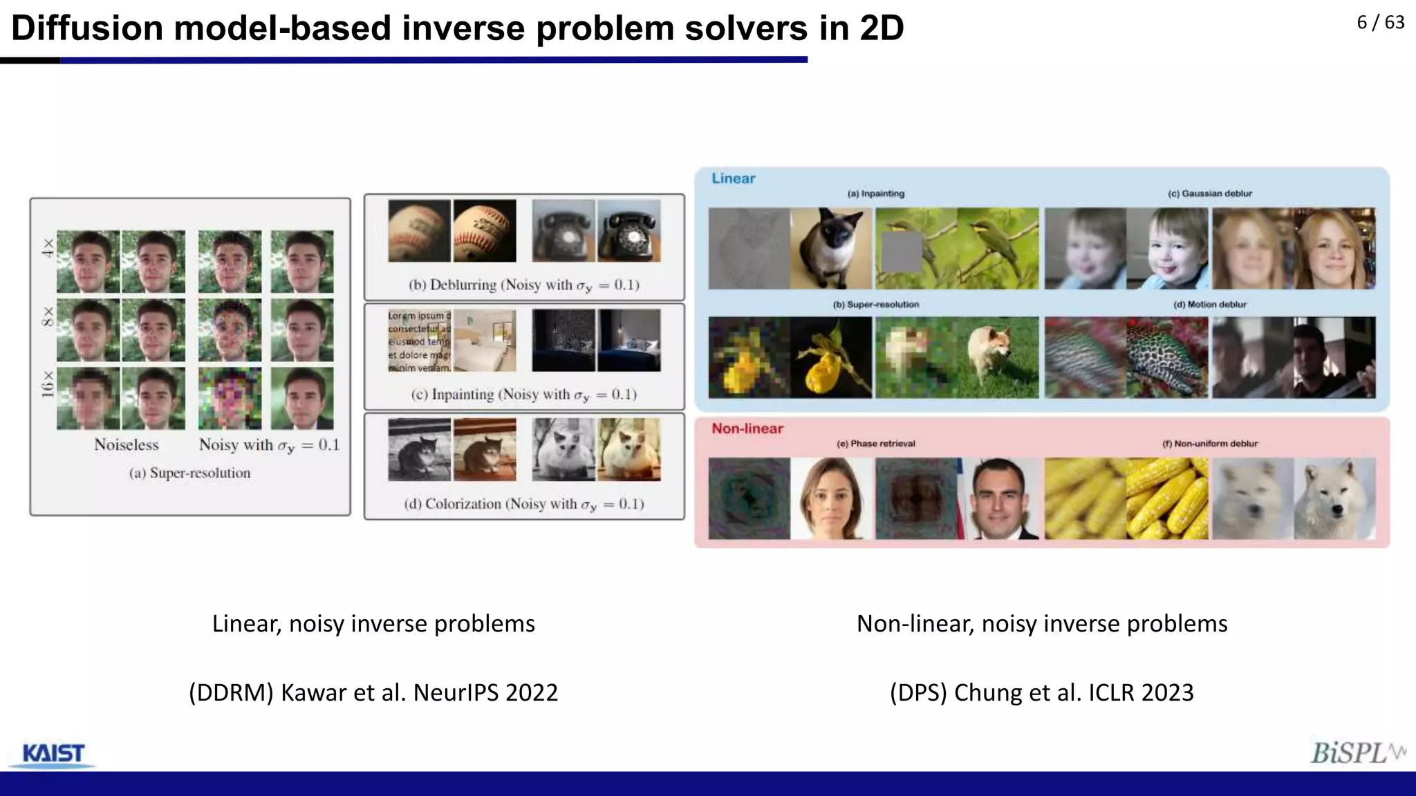
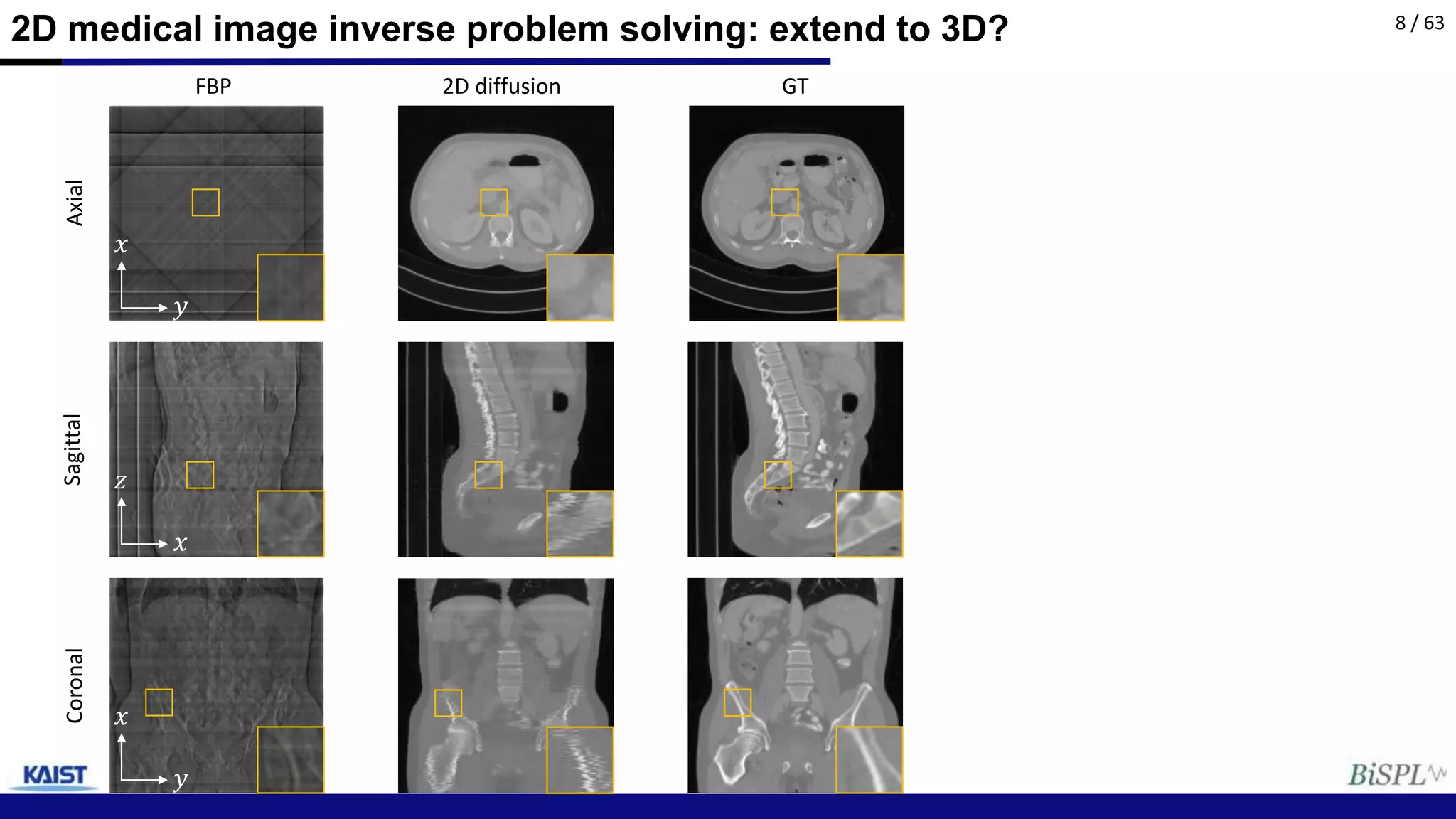
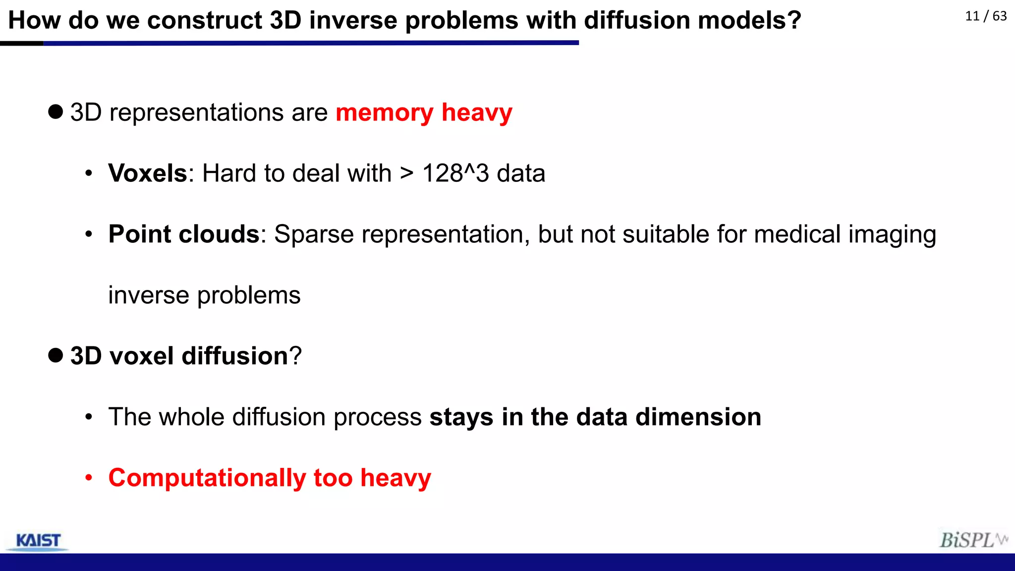
Solving 3D Inverse Problems using Pre-
trained 2D Diffusion Models
Dohoon Ryu Michael T. Mccann Marc L. Klasky Jong Chul Ye
1 / 63
Hyungjin Chung
CVPR 2023
http://yang-song.github.io/blog/2021/score/
Background: Diffusion models and Stein score
Explicit score matching
Denoising score matching
Equivalent (Vincent et al. 2010)
𝜽∗
= argmin
𝜽
𝔼[‖∇𝐱log 𝑝 𝐱 − 𝐬𝜽(𝐱)‖2
2
]
𝜽∗ = argmin
𝜽
𝔼[‖∇𝐱log 𝑝 𝐱 | 𝐱 − 𝐬𝜽(𝐱)‖2
2
]
2 / 63
http://yang-song.github.io/blog/2021/score/
Background: Diffusion models and Stein score 3 / 63
Background: Inverse problems
Imaging system
𝒜
𝐱
Ground truth image
𝜼
noise
𝐲
Measurement
• Problem: recover 𝐱 from noisy measurement 𝐲
• Ill-posed: Infinitely many solutions may exist
• We need to know the prior of the data distribution: how should the image look like?
4 / 63
Background: Examples of inverse problems in 2D
𝐲
𝐱
• Inpainting
⨀
• Deblurring (Deconvolution)
𝐱 𝐲
∗
• CS-MRI
𝓕
⨀
5 / 63
Diffusion model-based inverse problem solvers in 2D 6 / 63
(DPS) Chung et al. ICLR 2023
Non-linear, noisy inverse problems
(DDRM) Kawar et al. NeurIPS 2022
Linear, noisy inverse problems
2D medical image inverse problem solving 7 / 63
5
view
2D medical image inverse problem solving: extend to 3D? 8 / 63
Axial
Sagittal
Coronal
𝑥
𝑦
𝑧
𝑥
𝑥
𝑦
FBP 2D diffusion GT
2D medical image inverse problem solving: extend to 3D? 9 / 63
Axial
Sagittal
Coronal
𝑥
𝑦
𝑧
𝑥
𝑥
𝑦
FBP 2D diffusion GT
- Significant artifacts
- No dependency across
slices
3D inverse problems in medical imaging 10 / 63
How do we construct 3D inverse problems with diffusion models?
 3D representations are memory heavy
• Voxels: Hard to deal with > 128^3 data
• Point clouds: Sparse representation, but not suitable for medical imaging
inverse problems
 3D voxel diffusion?
• The whole diffusion process stays in the data dimension
• Computationally too heavy
11 / 63
Augmenting 2D diffusion prior with model-based prior
Model-based prior (TV) 𝑇𝑉 𝒙 ≔ 𝐷𝑥𝒙, 𝐷𝑦𝒙, 𝐷𝑧𝒙
1
Diffusion prior ∇𝒙log 𝑝(𝒙)
12 / 63
Augmenting 2D diffusion prior with model-based prior
Model-based prior (TV: z) 𝑇𝑉
z 𝒙 ≔ 𝐷𝑧𝒙 1
Diffusion prior (xy) ∇𝒙xy
log 𝑝(𝒙xy)
13 / 63
Augmenting 2D diffusion prior with model-based prior
1. Denoising with score function (parallel)
𝒙′𝑖−1 ← 𝜎𝑖
2
− 𝜎𝑖−1
2
𝒔𝜃∗ 𝒙𝑡, 𝑡 + 𝜎𝑖
2
− 𝜎𝑖−1
2
𝝐
2. Data consistency + TV prior augmenting (joint)
𝒙i−1 ← argmin
𝒙′𝑖−1
1
2
‖𝒚 − 𝑨𝒙′𝑖−1‖2
2
+ ‖𝑫𝒛𝒙′𝑖−1‖1
14 / 63
Augmenting 2D diffusion prior with model-based prior
1. Denoising with score function (parallel)
𝒙′𝑖−1 ← 𝜎𝑖
2
− 𝜎𝑖−1
2
𝒔𝜃∗ 𝒙𝑡, 𝑡 + 𝜎𝑖
2
− 𝜎𝑖−1
2
𝝐
2. Data consistency + TV prior augmenting (joint)
𝒙i−1 ← argmin
𝒙′𝑖−1
1
2
‖𝒚 − 𝑨𝒙′𝑖−1‖2
2
+ ‖𝑫𝒛𝒙′𝑖−1‖1
Effectively solved with, e.g. ADMM
15 / 63
Augmenting 2D diffusion prior with model-based prior 16 / 63
Fast DiffusionMBIR
Sharing primal/dual variables
• Warm start
• Much faster convergence
17 / 63
Sharing primal/dual variables
• Warm start
• Much faster convergence
Score update (denoising)
• Prior in 𝑥𝑦 dimension
Fast DiffusionMBIR 18 / 63
Sharing primal/dual variables
• Warm start
• Much faster convergence
Score update (denoising)
• Prior in 𝑥𝑦 dimension
ADMM-TV iteration
• Data consistency
• Prior in 𝑧 dimension
Fast DiffusionMBIR 19 / 63
Results (8-view sparse view reconstruction)
13.36 / 0.404 14.19 / 0.537 15.65 / 0.674
33.34 / 0.938 34.23 / 0.968 34.06 / 0.960
Coherent results across the whole volume
20 / 63
Results: All three problems 21 / 63
Thank you!

DiffusionMBIR_presentation_slide.pptx

  • 1.
    Solving 3D InverseProblems using Pre- trained 2D Diffusion Models Dohoon Ryu Michael T. Mccann Marc L. Klasky Jong Chul Ye 1 / 63 Hyungjin Chung CVPR 2023
  • 2.
    http://yang-song.github.io/blog/2021/score/ Background: Diffusion modelsand Stein score Explicit score matching Denoising score matching Equivalent (Vincent et al. 2010) 𝜽∗ = argmin 𝜽 𝔼[‖∇𝐱log 𝑝 𝐱 − 𝐬𝜽(𝐱)‖2 2 ] 𝜽∗ = argmin 𝜽 𝔼[‖∇𝐱log 𝑝 𝐱 | 𝐱 − 𝐬𝜽(𝐱)‖2 2 ] 2 / 63
  • 3.
  • 4.
    Background: Inverse problems Imagingsystem 𝒜 𝐱 Ground truth image 𝜼 noise 𝐲 Measurement • Problem: recover 𝐱 from noisy measurement 𝐲 • Ill-posed: Infinitely many solutions may exist • We need to know the prior of the data distribution: how should the image look like? 4 / 63
  • 5.
    Background: Examples ofinverse problems in 2D 𝐲 𝐱 • Inpainting ⨀ • Deblurring (Deconvolution) 𝐱 𝐲 ∗ • CS-MRI 𝓕 ⨀ 5 / 63
  • 6.
    Diffusion model-based inverseproblem solvers in 2D 6 / 63 (DPS) Chung et al. ICLR 2023 Non-linear, noisy inverse problems (DDRM) Kawar et al. NeurIPS 2022 Linear, noisy inverse problems
  • 7.
    2D medical imageinverse problem solving 7 / 63 5 view
  • 8.
    2D medical imageinverse problem solving: extend to 3D? 8 / 63 Axial Sagittal Coronal 𝑥 𝑦 𝑧 𝑥 𝑥 𝑦 FBP 2D diffusion GT
  • 9.
    2D medical imageinverse problem solving: extend to 3D? 9 / 63 Axial Sagittal Coronal 𝑥 𝑦 𝑧 𝑥 𝑥 𝑦 FBP 2D diffusion GT - Significant artifacts - No dependency across slices
  • 10.
    3D inverse problemsin medical imaging 10 / 63
  • 11.
    How do weconstruct 3D inverse problems with diffusion models?  3D representations are memory heavy • Voxels: Hard to deal with > 128^3 data • Point clouds: Sparse representation, but not suitable for medical imaging inverse problems  3D voxel diffusion? • The whole diffusion process stays in the data dimension • Computationally too heavy 11 / 63
  • 12.
    Augmenting 2D diffusionprior with model-based prior Model-based prior (TV) 𝑇𝑉 𝒙 ≔ 𝐷𝑥𝒙, 𝐷𝑦𝒙, 𝐷𝑧𝒙 1 Diffusion prior ∇𝒙log 𝑝(𝒙) 12 / 63
  • 13.
    Augmenting 2D diffusionprior with model-based prior Model-based prior (TV: z) 𝑇𝑉 z 𝒙 ≔ 𝐷𝑧𝒙 1 Diffusion prior (xy) ∇𝒙xy log 𝑝(𝒙xy) 13 / 63
  • 14.
    Augmenting 2D diffusionprior with model-based prior 1. Denoising with score function (parallel) 𝒙′𝑖−1 ← 𝜎𝑖 2 − 𝜎𝑖−1 2 𝒔𝜃∗ 𝒙𝑡, 𝑡 + 𝜎𝑖 2 − 𝜎𝑖−1 2 𝝐 2. Data consistency + TV prior augmenting (joint) 𝒙i−1 ← argmin 𝒙′𝑖−1 1 2 ‖𝒚 − 𝑨𝒙′𝑖−1‖2 2 + ‖𝑫𝒛𝒙′𝑖−1‖1 14 / 63
  • 15.
    Augmenting 2D diffusionprior with model-based prior 1. Denoising with score function (parallel) 𝒙′𝑖−1 ← 𝜎𝑖 2 − 𝜎𝑖−1 2 𝒔𝜃∗ 𝒙𝑡, 𝑡 + 𝜎𝑖 2 − 𝜎𝑖−1 2 𝝐 2. Data consistency + TV prior augmenting (joint) 𝒙i−1 ← argmin 𝒙′𝑖−1 1 2 ‖𝒚 − 𝑨𝒙′𝑖−1‖2 2 + ‖𝑫𝒛𝒙′𝑖−1‖1 Effectively solved with, e.g. ADMM 15 / 63
  • 16.
    Augmenting 2D diffusionprior with model-based prior 16 / 63
  • 17.
    Fast DiffusionMBIR Sharing primal/dualvariables • Warm start • Much faster convergence 17 / 63
  • 18.
    Sharing primal/dual variables •Warm start • Much faster convergence Score update (denoising) • Prior in 𝑥𝑦 dimension Fast DiffusionMBIR 18 / 63
  • 19.
    Sharing primal/dual variables •Warm start • Much faster convergence Score update (denoising) • Prior in 𝑥𝑦 dimension ADMM-TV iteration • Data consistency • Prior in 𝑧 dimension Fast DiffusionMBIR 19 / 63
  • 20.
    Results (8-view sparseview reconstruction) 13.36 / 0.404 14.19 / 0.537 15.65 / 0.674 33.34 / 0.938 34.23 / 0.968 34.06 / 0.960 Coherent results across the whole volume 20 / 63
  • 21.
    Results: All threeproblems 21 / 63
  • 22.

Editor's Notes

  • #2 So far we’ve considered noisy, non-linear, and blind. Our final piece will be to apply 2D diffusion to 3D inverse problems, especially in the context of medical imaging.
  • #3 In order to circumvent the intractable explicit score matching, you train your network with denoising score matching, which boils down to essentially training a residual denoiser.
  • #4 Another interesting view is that one can view the data noising process as some linear forward SDE, and the data generating process as the corresponding reverse SDE, where the drift function is governed by the score function. Hence, when you want to sample data, you can discretize the reverse SDE and numerically solve it using the pre-trained score function.
  • #5 On the other hand, we are interested in solving inverse problems. In the inverse problem setting, our aim is to recover the grond truth x from the noisy measurement y, obtained through some integral imaging system A, polluted with the measurement noise n. The problem is naturally ill-posed, which means that there exists infinitely many solutions to this problem. Hence, in order to correctly specify which one of the solutions is the one that we want, we need to specify the prior of the data distribution, in other words, how the images looks like.
  • #6 Examples of such inverse problems include inpainting, deconvolution, and compressed sensing MRI.
  • #7 Examples of such inverse problems include inpainting, deconvolution, and compressed sensing MRI.
  • #11 By 3D inverse problem, we can think of the following three representative examples. In the left, we have limited angle CT, where we only have measurements in the limited green angles. Sparse view CT considers the case where we have very few projections at hand, for example 4-view CT. Finally, compressed sensing MRI of 3D volumes is also the case of 3D inverse problem.
  • #12 To first look at why this problem is even interesting in the first place, one should note that there is no representation that everybody uses for 3D data. For 2D images, we do have a consensus, use discretized matrices to represent image. For 3D, using voxels isn’t so desirable in many use cases. It’s just too memory inefficient, and tends to be very heavy if we try to scale over 128 cubed resolution. These are the main reasons that the computer vision folks like to use meshes, point clouds, or more recently neural fields. However, using representations other than voxels are not suitable for medical imaging inverse problems, when seeing the interior of the 3D volume is of absolute necessity. Well, then can we use 3D voxel diffusion? The answer is absolutely not, since the diffusion model is already computationally too heavy with 2D diffusion, and our tiny GPUs would not be able to handle such massive memory.
  • #13 So our proposal is to leave 2D diffusion as is, and try to incorporate lessons from the more classic literature. Specifically, we bring the total variation prior, which essentially states that natural images tend to have sparse gradients.
  • #14 In particular, we choose to impose TV only to the redundant z-direction, as for xy dimension, the diffusion prior pretty much covers it all. Apologies for the sloppy notation, but I think you can get the point.
  • #15 We can implement our idea as follows. First, we denoise each slice with 2D score functions in parallel. If we only use step 1 iteratively, we get slices that are independent of each other, such that when seen from the coronal or the sagittal slices, they are incoherent. Hence, in the second step, we aggregate the slices to form the volume, and minimize the following sub-problem, which imposes both the data consistency condition, and the TV prior to the z-direction.
  • #16 The optimization can be performed effectively, with for example, ADMM.
  • #17 We can visualize our method as follows. However, if we were to naively implement this approach, it would mean that we would have to run the ADMM steps per every iteration, which would be infeasible.
  • #18 Hence, we propose another strategy called variable sharing, in which we treat all the primal and the dual variables of ADMM as global variables that are shared through the whole reverse diffusion process. This would mean that we are warm-starting all the ADMM and the CG steps in-between, which will lead to much faster convergence with limited number of steps.
  • #19 So like I explained with the figure, we first denoise with the score function,
  • #20 And then we’ll apply ADMM-TV, but we will run a single sweep of ADMM, with a single sweep of CG. You might think that there’s no way that this is going to converge, but it does, since we can slowly update the estimates during the reverse diffusion process.
  • #21 With the proposed method, we are able to achieve reconstructions from extremely limited number of views.
  • #22 In the paper, we show that we can apply this same methodology to all the three problems, including sparse-view tomography, limited-angle tomography, and compressed sensing MRI.
  • #23 So far we’ve considered noisy, non-linear, and blind. Our final piece will be to apply 2D diffusion to 3D inverse problems, especially in the context of medical imaging.