


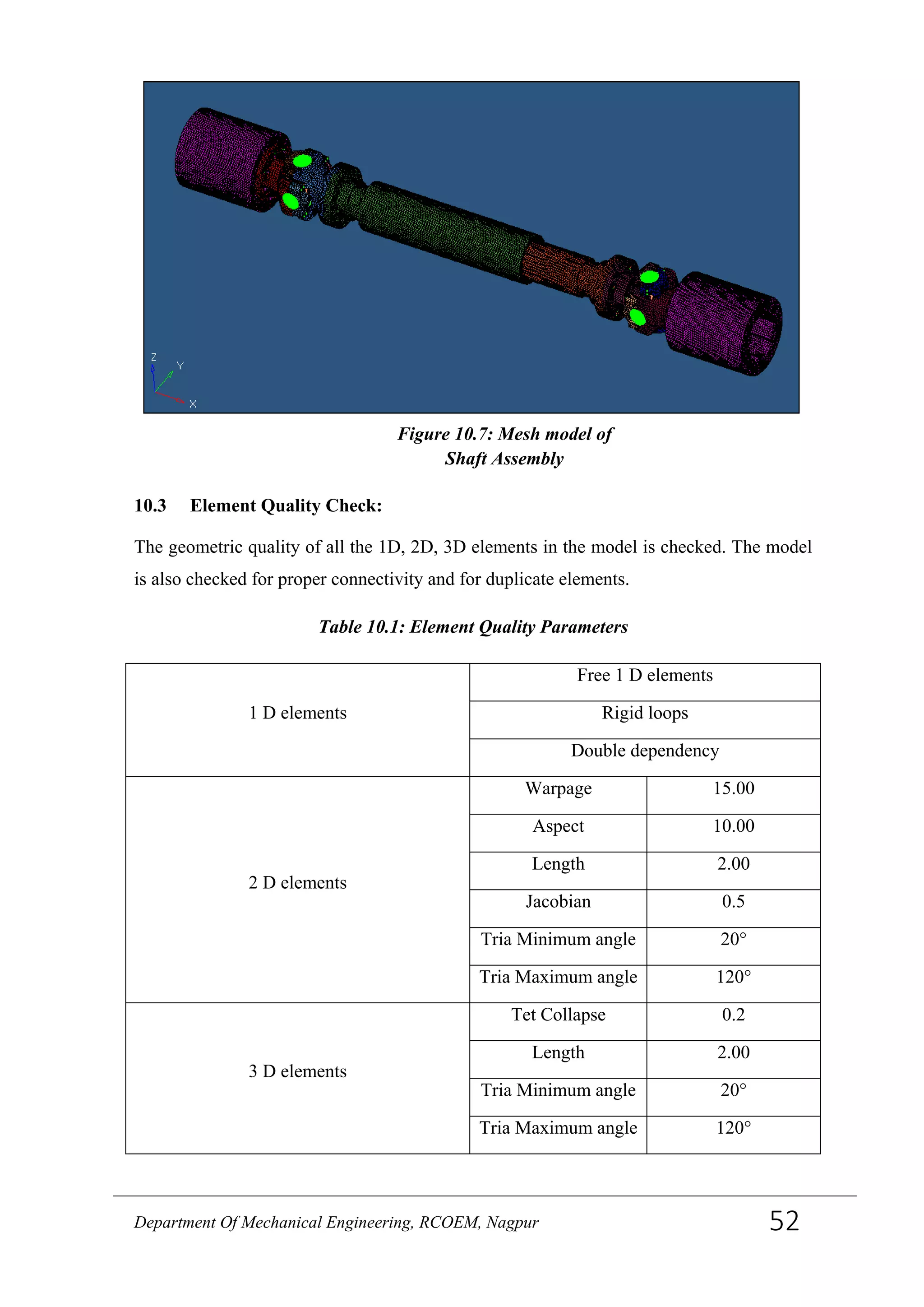
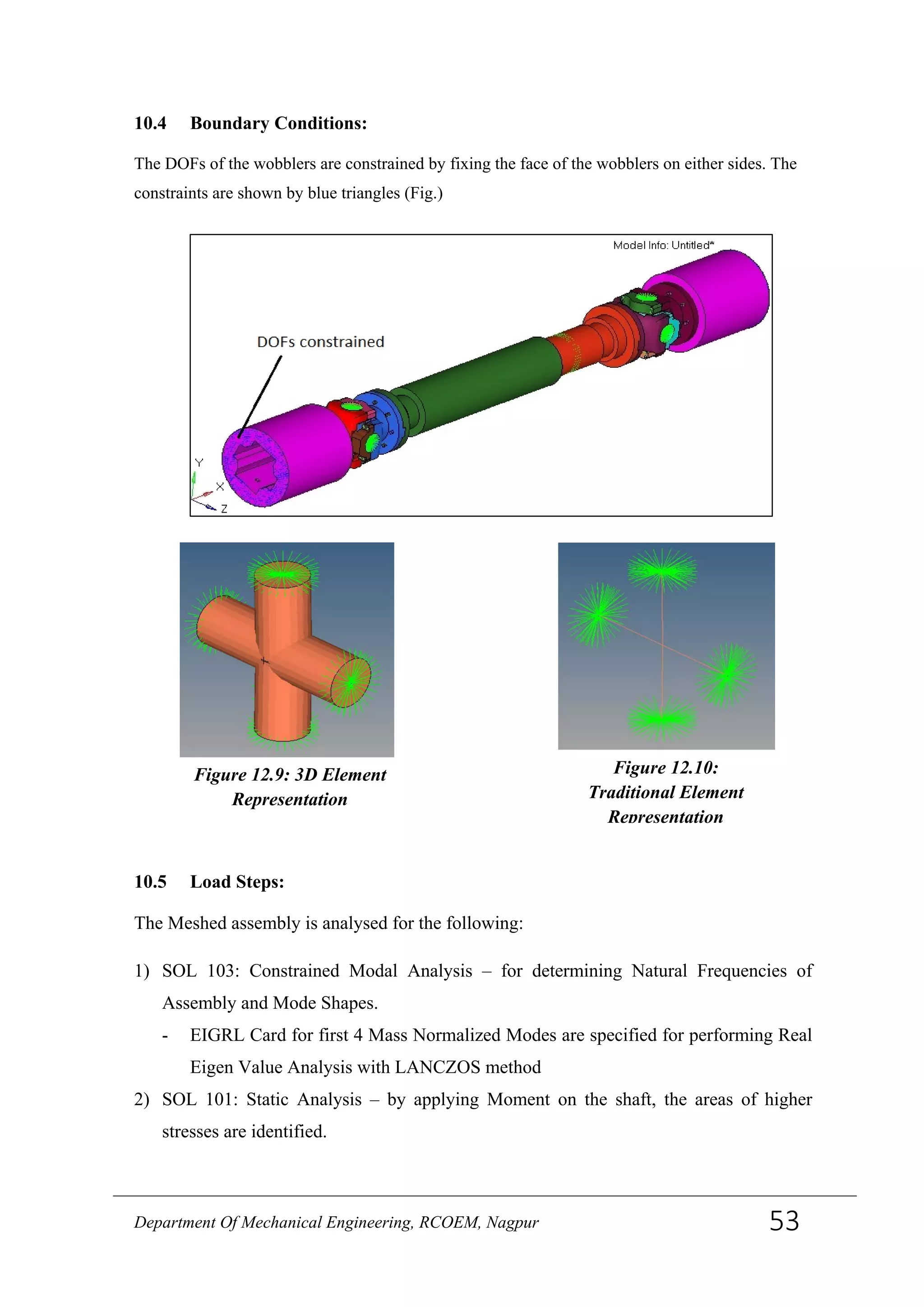
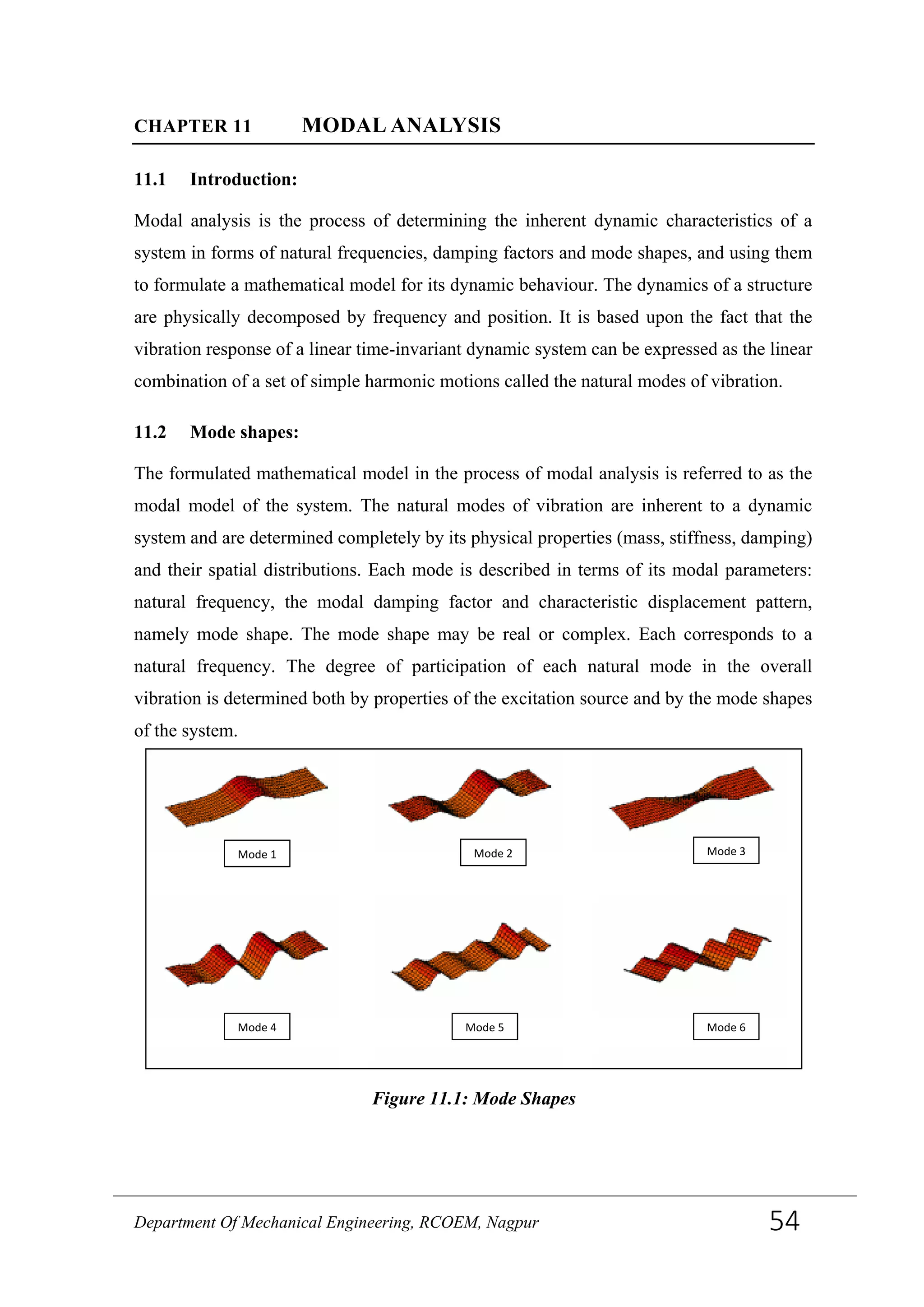
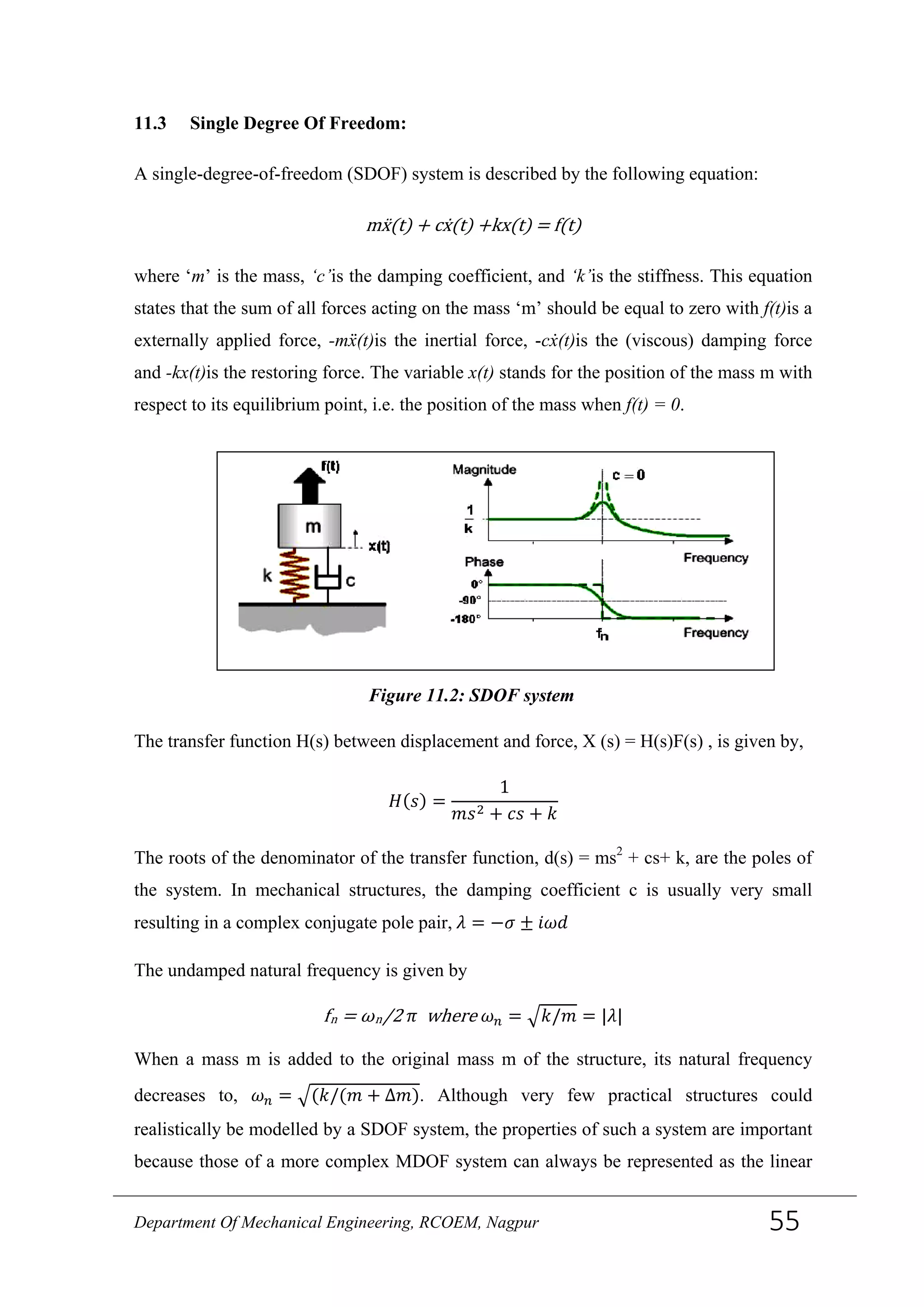
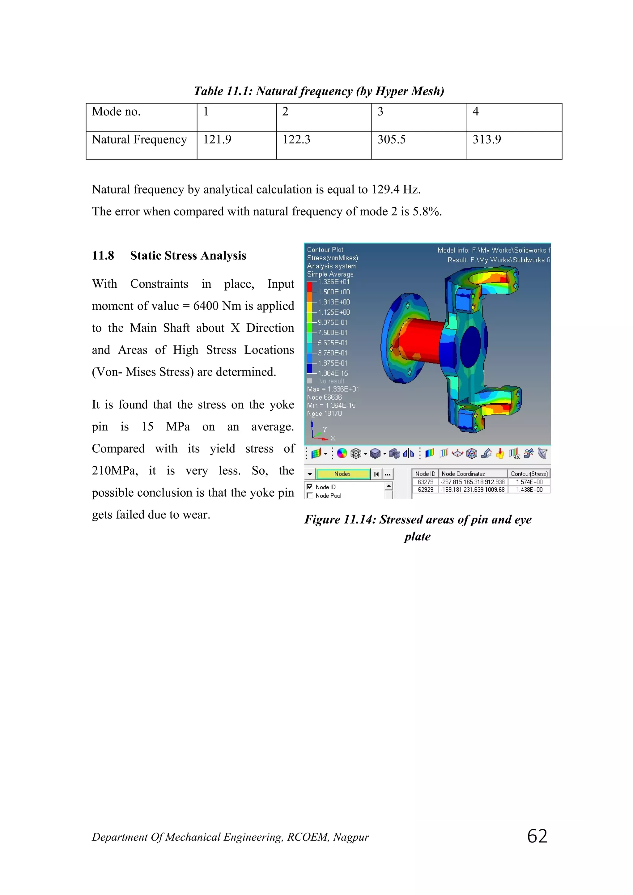
![CHAPTER 01 UNIVERSAL JOINT
1.1 Introduction
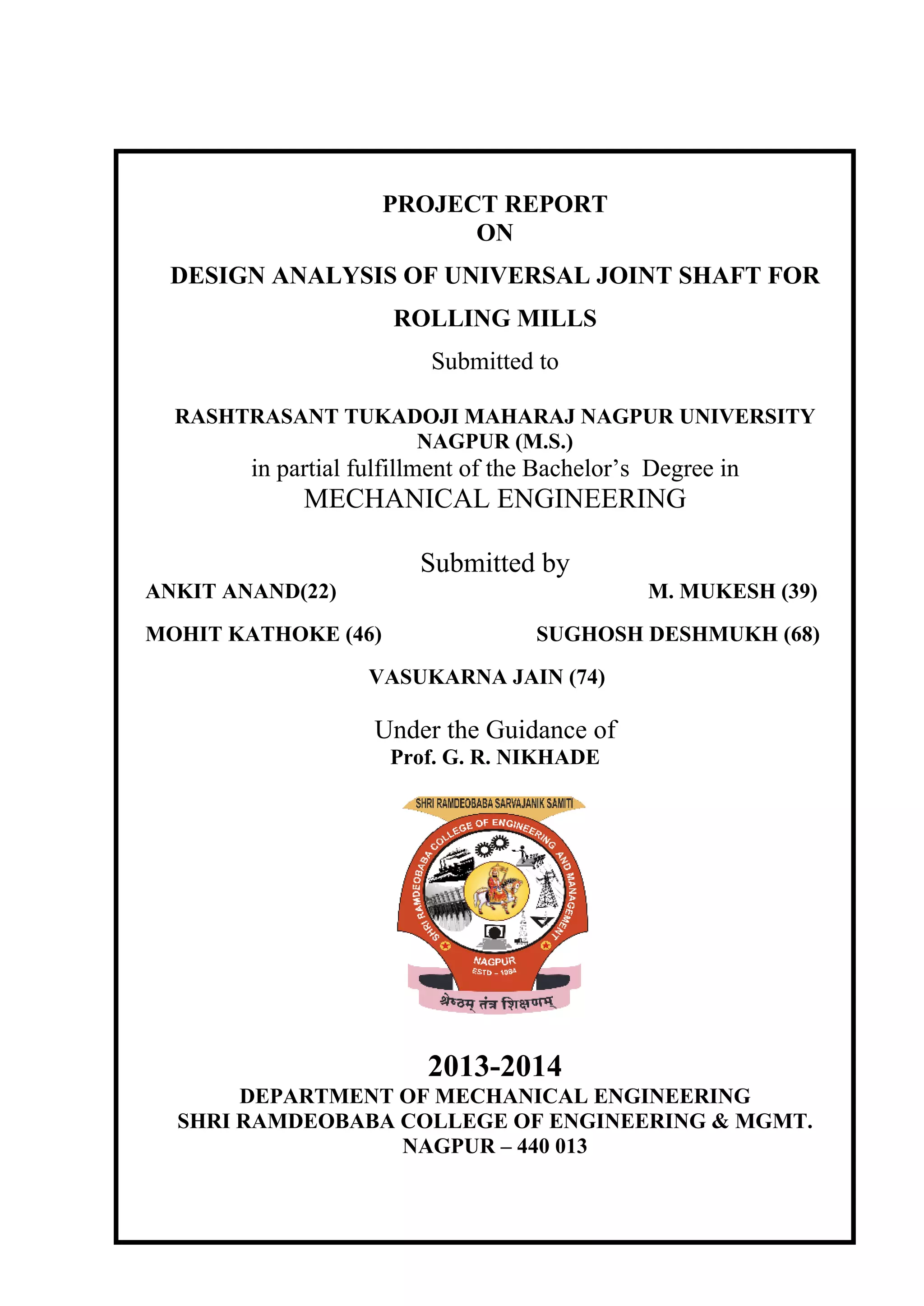
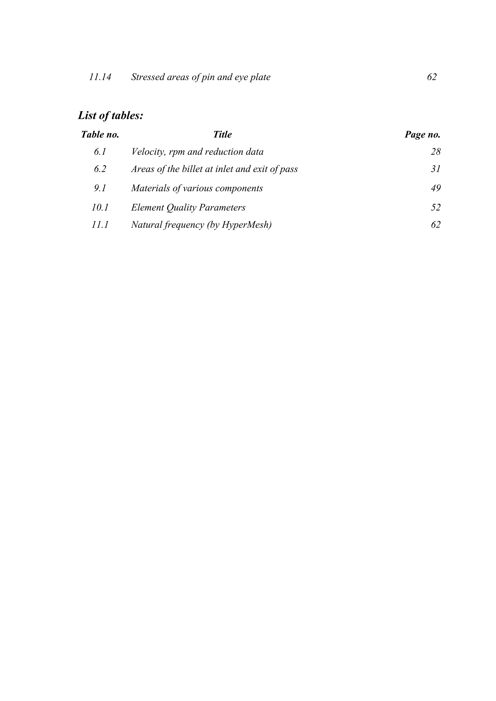
A universal joint, also known as universal coupling, U-joint, Cardan joint, Hardy
Spicer joint, or Hooke's joint is a joint or coupling in a rigid rod that allows the rod to
'bend' in any direction, and is commonly used in shafts that transmit rotary motion. It
consists of a pair of hinges located close together, oriented at 90° to each other, connected
by a cross shaft.
The term universal joint was used in the 18th
century and was in common use in the 19th
century. Edmund Morewood's 1844 patent for a metal coating machine called for a
universal joint, by that name, to accommodate small alignment errors between the engine
and rolling mill shafts. Lardner's 1877 Handbook described both simple and double
universal joints, and noted that they were much used in the line shaft systems of cotton
mills. Jules Weisbach described the mathematics of the universal joint and double
universal joint in his treatise on mechanics published in English in 1883.
19th
century uses of universal joints spanned a wide range of applications. Numerous
universal joints were used to link the control shafts of the Northumberland telescope at
Cambridge University in 1843. Ephriam Shay's locomotive patent of 1881, for example,
used double universal joints in the locomotive's drive shaft. Charles Amidon used a much
smaller universal joint in his bit-brace patented 1884. Beauchamp Tower's spherical,
rotary, high speed steam engine used an adaptation of the universal joint circa 1885.[1]
Figure 1.1: Universal Joint
Department Of Mechanical Engineering, RCOEM, Nagpur 1](https://image.slidesharecdn.com/projectreport-140702000203-phpapp02/75/DESIGN-ANALYSIS-OF-UNIVERSAL-JOINT-SHAFT-FOR-ROLLING-MILLS-10-2048.jpg)

![CHAPTER 02 LITERATURE REVIEW
To understand the scope of the project, the literature survey is a must. The literature
survey for this project is as follows.
2.1 Introduction
Robert Hooke is commonly thought of as the inventor of ‘Hooke's joint’ or the ‘universal
joint’. However, it is shown that this flexible coupling (based on a four-armed cross
pivoted between semi-circulars yoke attached to two shafts) was in fact known long before
Hooke's time but was always assumed to give an output exactly matching that of the input
shaft. Hooke carefully measured the relative displacements of the two axes, and found that
if one were inclined to the other, uniform rotation of the input produced a varying rate of
rotation of the output. Hooke's studies of the universal joint caused it to be identified with
his name, and it has ultimately proved far more important as a rotary coupling than as a
sundial analogue. More complex versions subsequently designed by Hooke included
provision for two basic couplings to be linked by an intermediate shaft. With appropriate
setting of phase and shaft angles this ‘double Hooke's joint’ could annul the variable
output velocity characteristic of the single universal. It has proved invaluable for modern
automotive transmissions.[20]
2.2 Angled couplings
Before proceeding further with applications of this device it is necessary to look back to an
earlier phase in the history of mechanisms. The need to transmit a rotary motion from a
primary shaft to a second shaft at an angle to the first (rather than directly in line or
parallel to it must have arisen repeatedly since ancient times, and been solved by a number
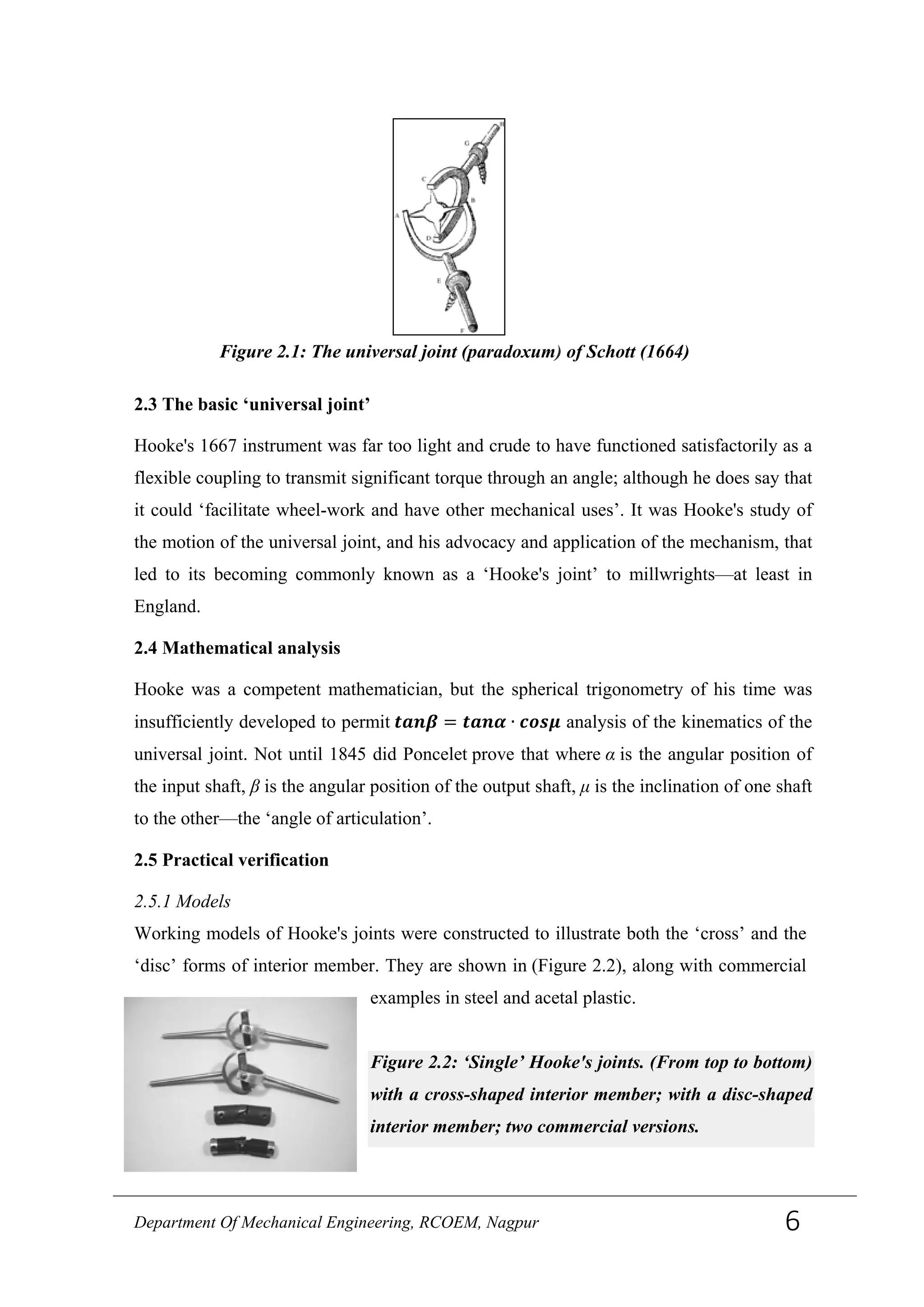
of anonymous artisans. An example cited by the Jesuit father Gaspar Schott was the 1354
clock in Strasbourg Cathedral, where the dial face was situated some way above and to the
side of the driving mechanism. Schott explains in a work published in 1664 that an angled
drive could have been achieved with bevel gears, but was more simply accomplished with
a chain of devices individually known as a paradoxum. He illustrates this mechanism with
the woodcut crediting it to an unpublished manuscript Chronometria Mechanica Nova by
a deceased anonymous author identified only as ‘Amicus’. The paradoxum can be seen to
be made up of the same two forks linked by a four-armed cross that characterize Hooke's
‘universal’.
Department Of Mechanical Engineering, RCOEM, Nagpur 5](https://image.slidesharecdn.com/projectreport-140702000203-phpapp02/75/DESIGN-ANALYSIS-OF-UNIVERSAL-JOINT-SHAFT-FOR-ROLLING-MILLS-14-2048.jpg)
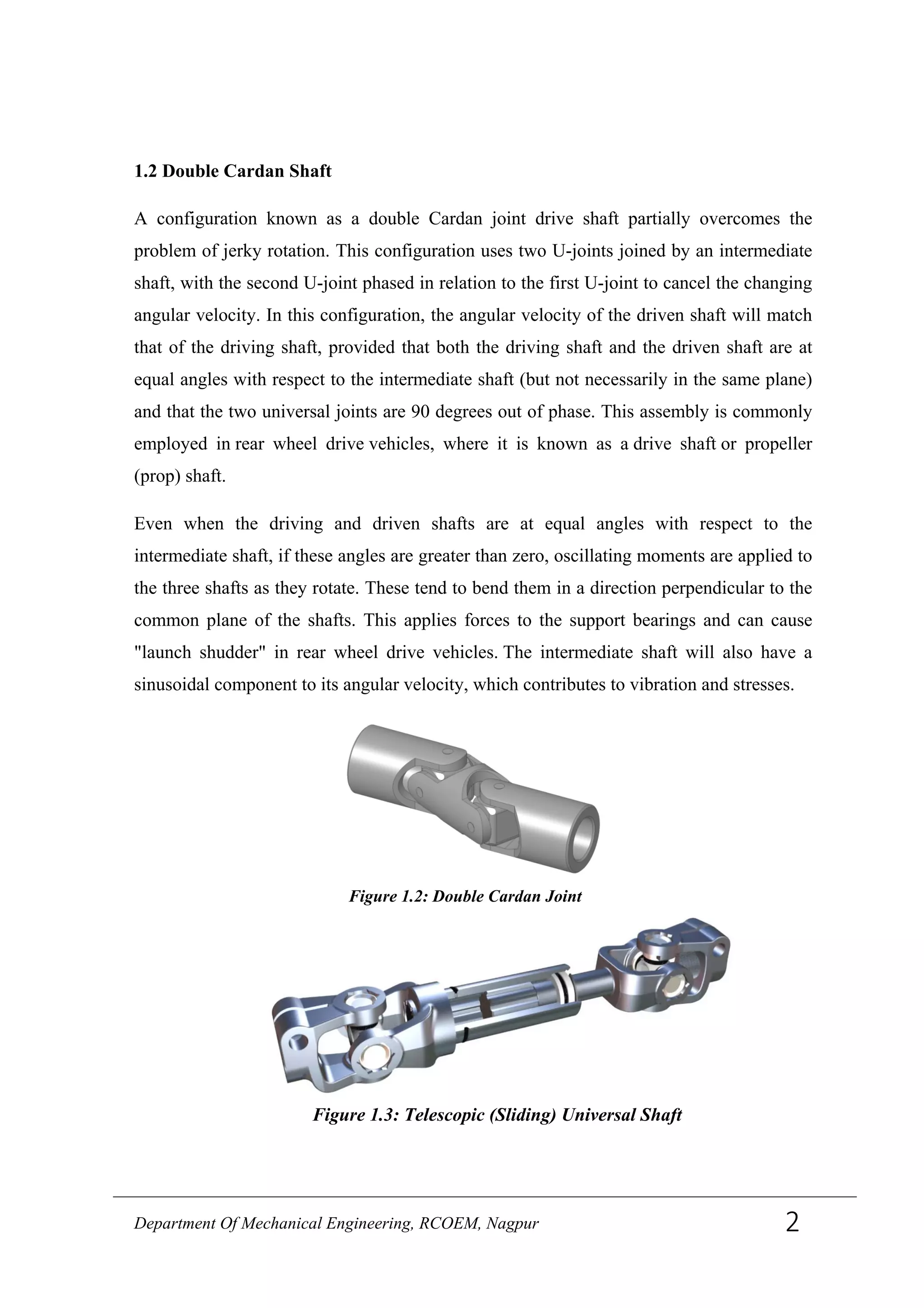
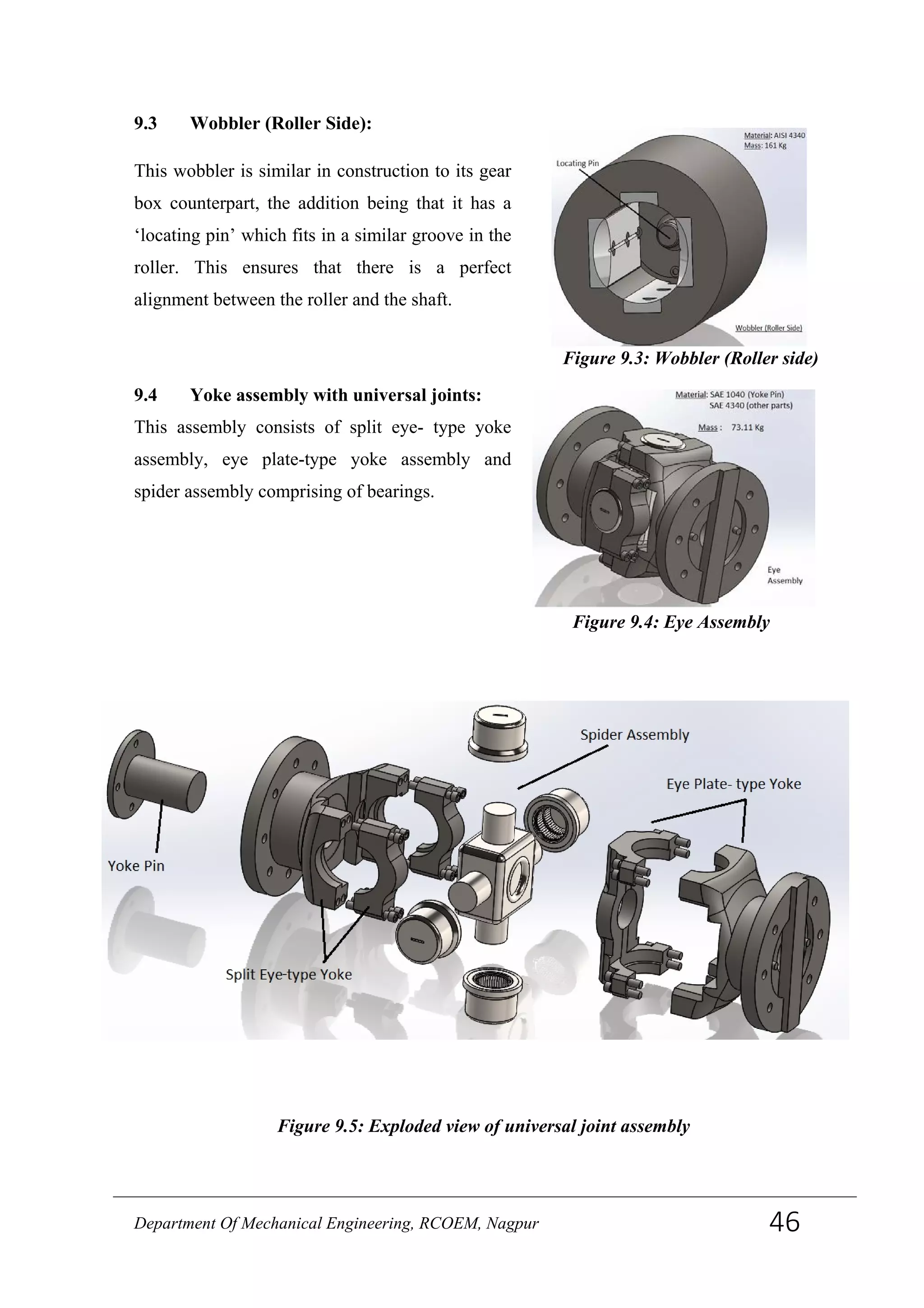
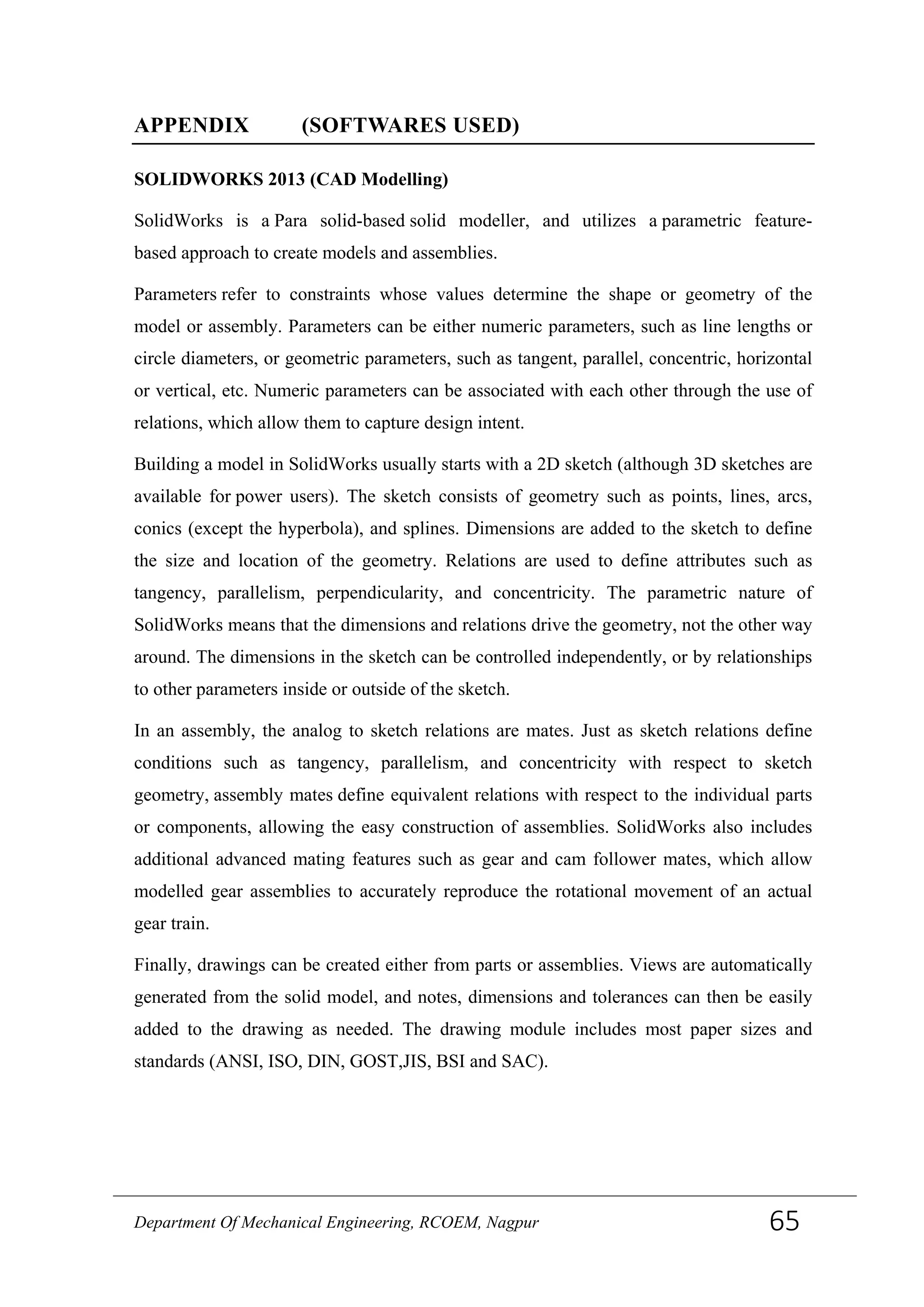
![bearing loading. Corrosion issues associated with split bearing eye designs are also
avoided. The 2-piece yokes and block type designs were developed to increase the cross
trunnion diameter and torque capacity of the U-joint while allowing for assembly. Split –
yoke designs are unique since the tie bolt is not used for torque transmission or retention
of yoke components after installation. All designs have the option of splined centre
sections to allow for length compensation for axial travel and alignment changes during
operation. Splines can be hardened, typically by nitriding, for applications with frequent
axial travel. The centre sections can be tubes welded directly to the yokes or flanged to
allow for more economical replacement sparing of U-joint parts. It is uncommon to
machine integral face pads or special spline teeth between the flange faces (Fig.9 and 10)
on high load applications. [19]
2.11 General Considerations in shaft design.
2.11.1 To minimize both deflections and stresses, the shaft length should be kept as short
as possible and overhangs minimized.
1.11.2. A cantilever beam will have a larger deflection than a simply supported (straddle
mounted) one for the same length, load, and cross section, so straddle mounting should be
used unless a cantilever shaft is dictated by design constraints.
1.11.3. A hollow shaft has a better stiffness/mass ratio (specific stiffness) and higher
natural frequencies than a comparably stiff or strong solid shaft, but will be more
expensive and larger in diameter.
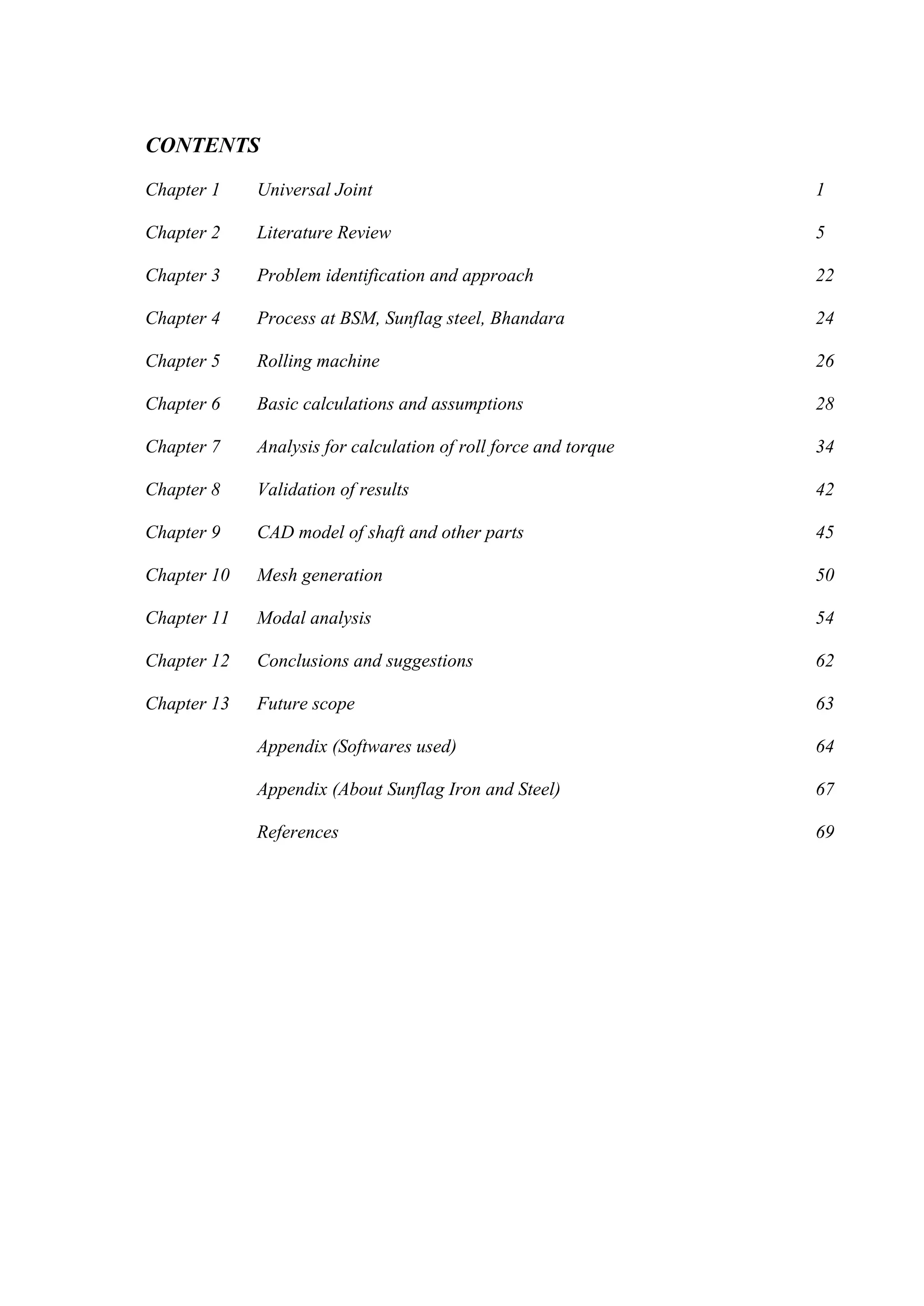
Figure 2.15: Radial face spline.Figure 2.14: Integral face pads
Department Of Mechanical Engineering, RCOEM, Nagpur 14](https://image.slidesharecdn.com/projectreport-140702000203-phpapp02/75/DESIGN-ANALYSIS-OF-UNIVERSAL-JOINT-SHAFT-FOR-ROLLING-MILLS-23-2048.jpg)

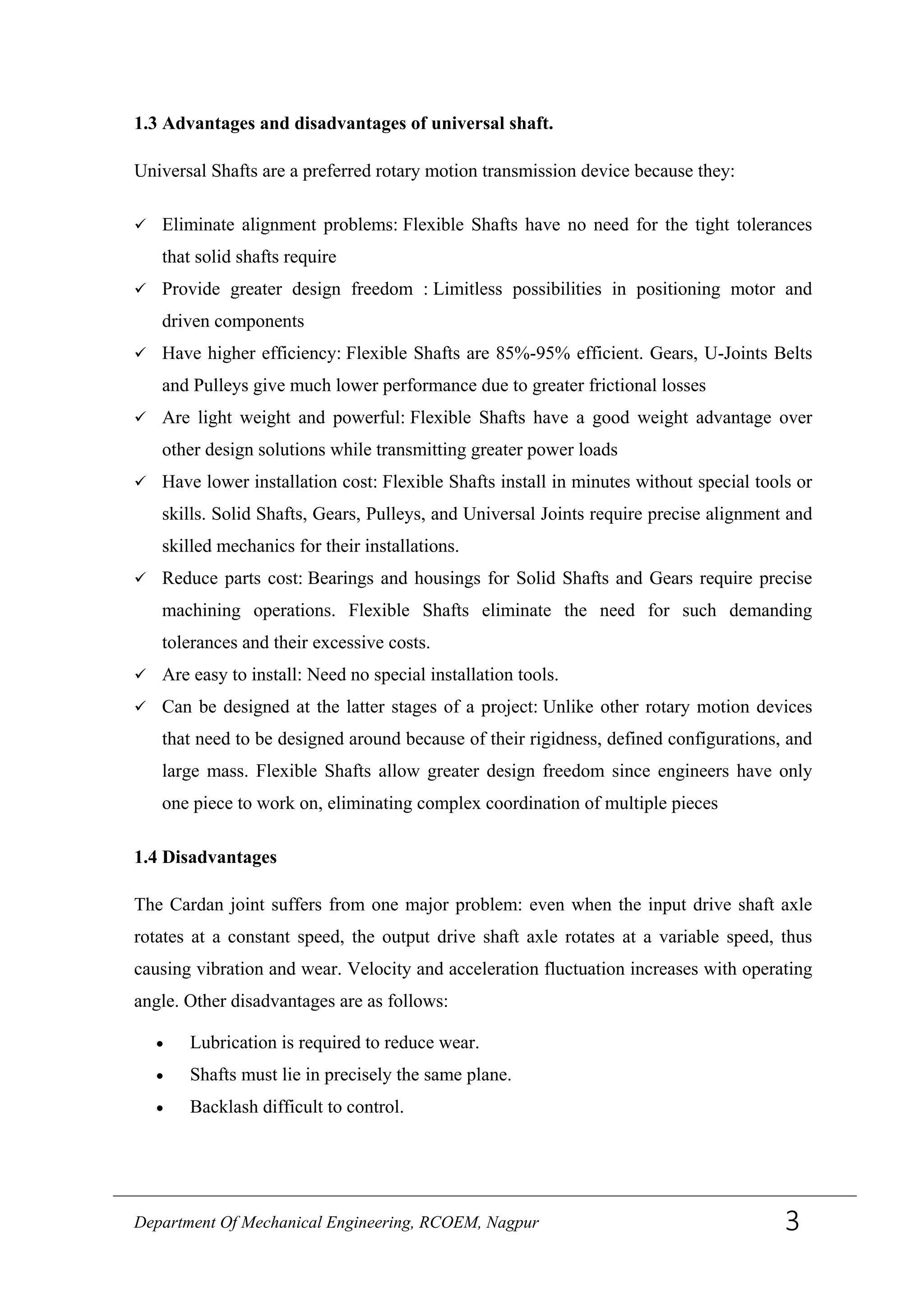
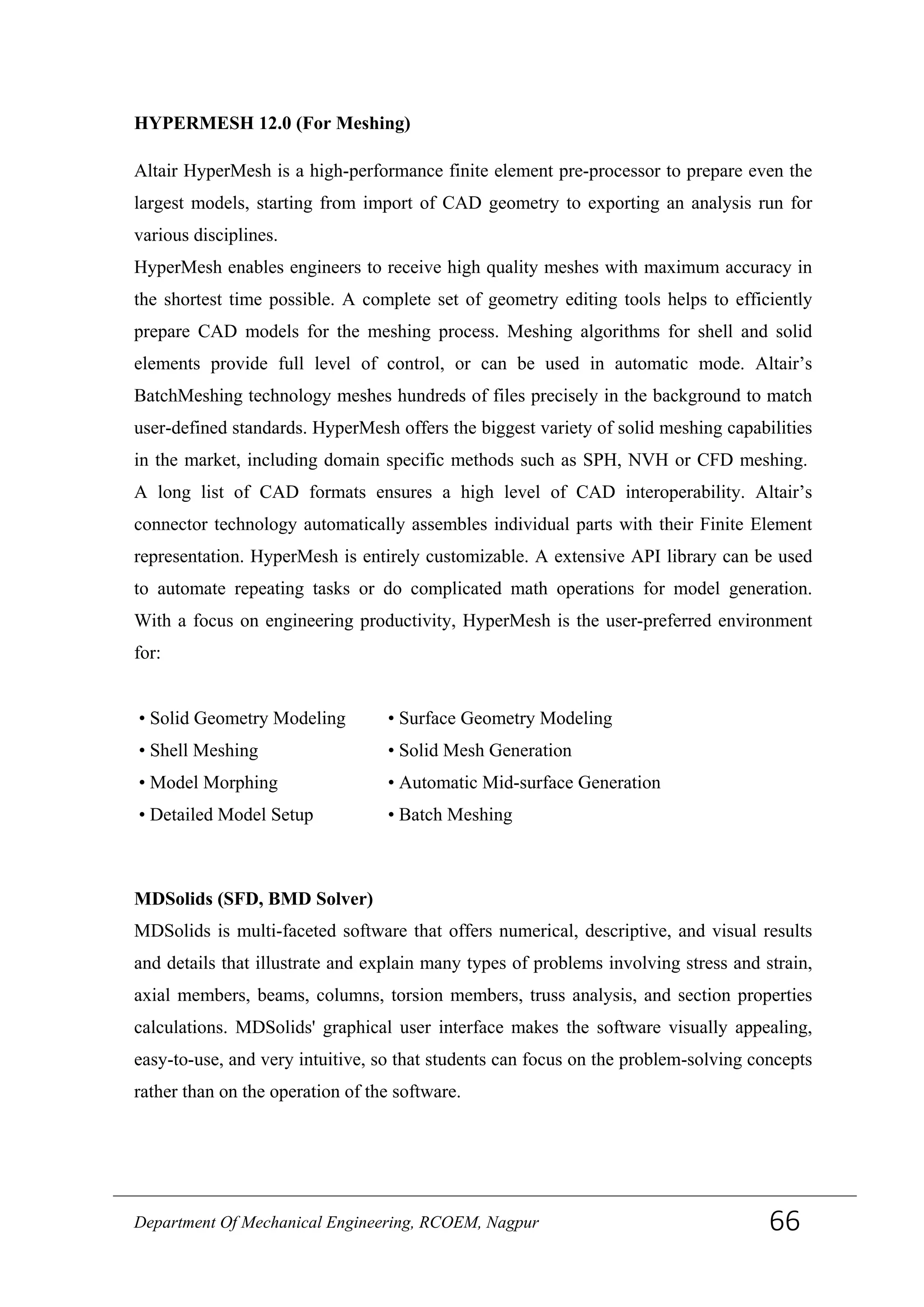
![2.13.1Factors for the Torque Rating of Universal Joints [23]
2.14 Selection criteria
2.14.1 Torque requirements:
The first step in selecting a Cardan shaft is determining the maximum torque to be
transmitted. The maximum torque should take into account the maximum prime mover
torque including inertial effects from the prime mover when decelerating during
overloads. The prime mover torque is generally considered as being unequally split
through the pinion stand in the range of 40 to 67% to allow for unequal torque loading of
the mill rolls.
This application torque is adjusted by applying the appropriate service factor(s) in
accordance with the joint manufacturer’s recommendation. The resultant selection torque
is compared to either: the U-joint’s endurance or fatigue torque rating for reversing
applications; or the one Way or pulsating fatigue torque rating for non-reversing
applications. Both the ratings are based on the material strength of shaft. The one way
torque rating is typically 1.5 times the reversing fatigue torque rating.
2.14.2 Maximum bending moment
During joint operation bending moment occur in the connecting shaft as function of
operating misalignment angle and driving torque. This bending moment causes a load on
supporting bearing that is periodic with two complete cycles per revolution of shaft. The
bending moment is always in plane of the ears of the yoke. The maximum value of
bending moment is given by
M = T tan (α)
Where, M = maximum bending moment
Department Of Mechanical Engineering, RCOEM, Nagpur 18](https://image.slidesharecdn.com/projectreport-140702000203-phpapp02/75/DESIGN-ANALYSIS-OF-UNIVERSAL-JOINT-SHAFT-FOR-ROLLING-MILLS-27-2048.jpg)


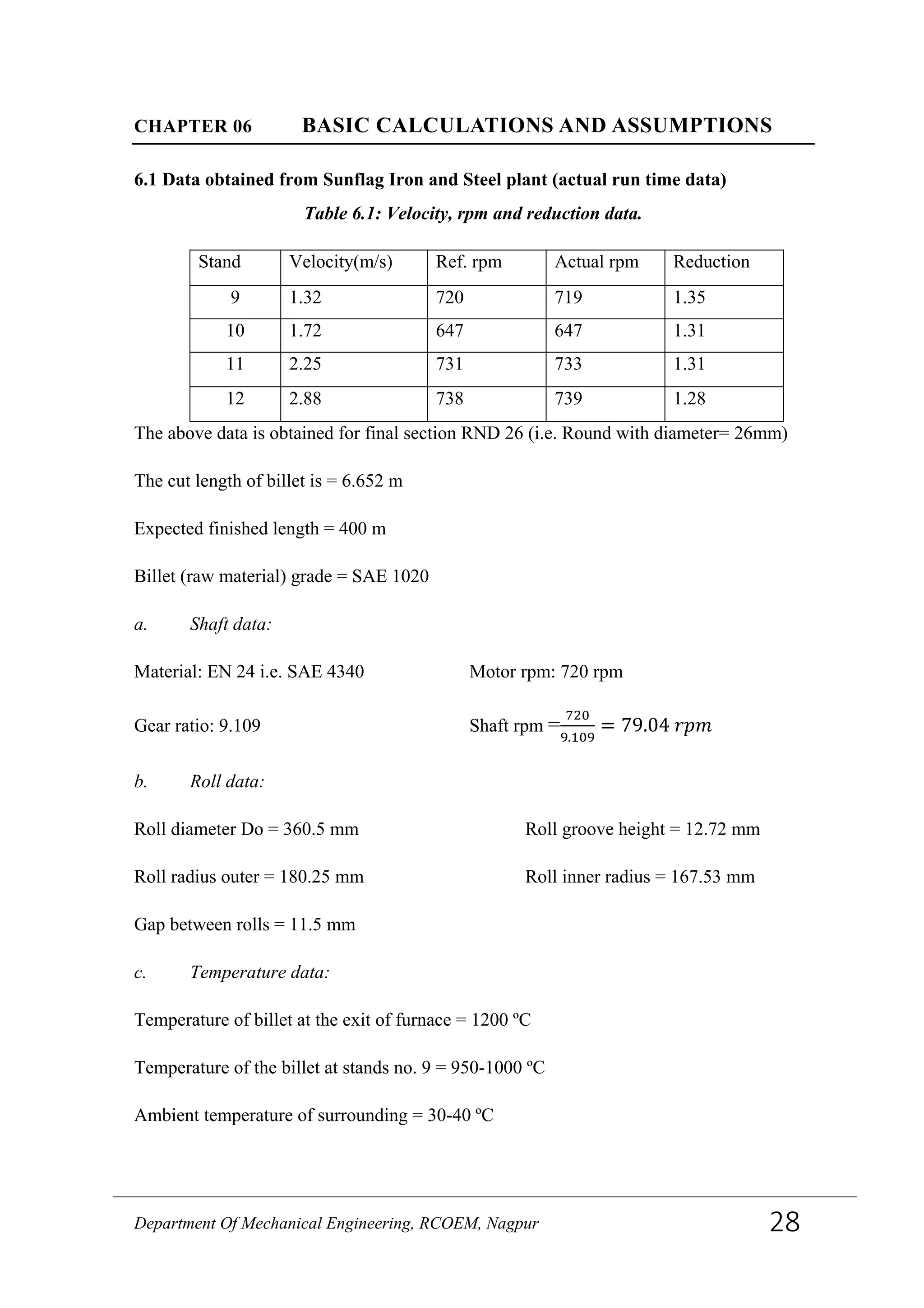
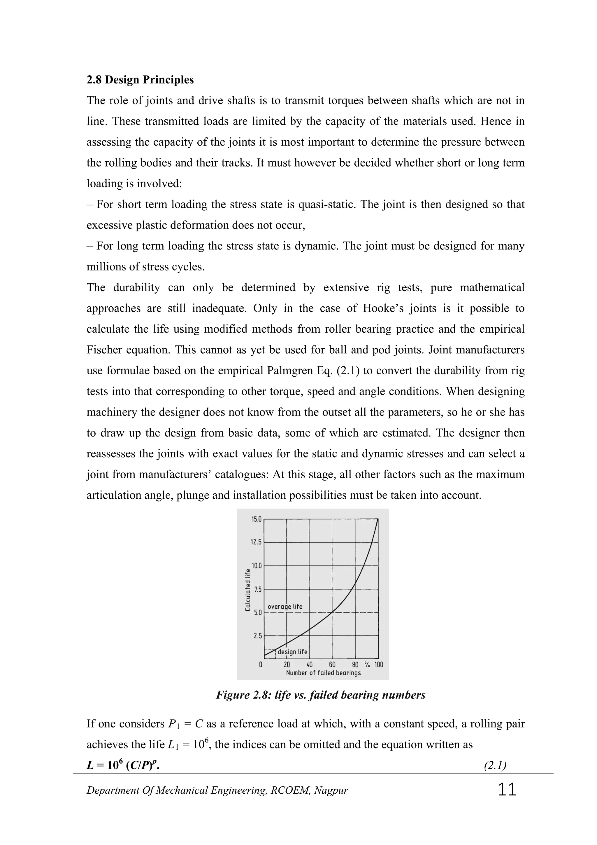
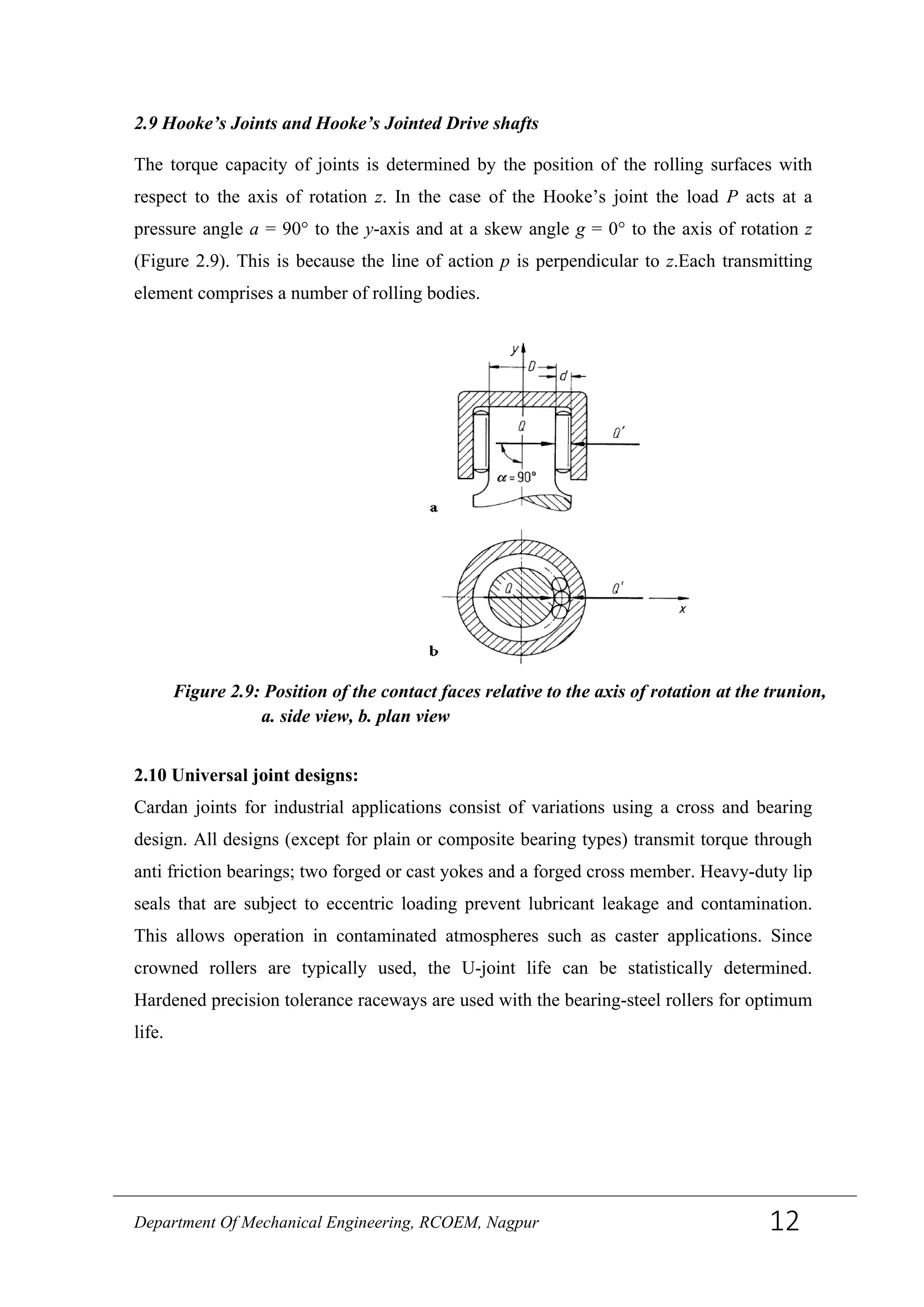
![6.2 Basic assumption
The rolling setup considered for this project is a bar mill for hot rolling of steels. To create
a closed form expression for the roll torque in rod rolling is very difficult. The governing
differential equation is much more complicated than in flat rolling since the stress state no
longer can be regarded as two dimensional. The geometry of the roll pass is more complex
to describe and all the other aspects such as describing the amount of inhomogeneous
deformation, interfacial friction etc. is also present in rod rolling. The traditional approach
is to relate the round or oval bar into an equivalent square section and then use some
analytic expression for flat rolling. Since the expressions for the roll torque in flat rolling
are not very accurate, one cannot expect these expressions combined with equivalent
rectangle methods to perform well. Another approach to try to adopt the flat rolling
expressions into rod rolling was introduced by Y. Lee and Y.H. Kim. In their study of the
roll force they introduce the weak plane-strain concept in order to produce a closed form
expression for the roll force. Since the strain in lateral direction in rod rolling is
constrained by the groove radius Lee and Kim argues that the stress state can be regarded
to be in a weak plane condition. They introduce a simple linear function to compensate for
the three-dimensional stress state in the roll gap in rod rolling. The pressure in rod rolling
is then presented as:
𝒑 𝒓𝒐𝒅 = (𝟏 − 𝜺 𝟏)𝒑 𝒑𝒍𝒂𝒏𝒆 𝒔𝒕𝒓𝒂𝒊𝒏
Where, ε1 is the lateral strain. An equivalent rectangle method is used to calculate average
effective strain and strain rate. They conduct an evaluation of their expression to measured
values from one round to oval and one oval to round pass at different temperatures. The
average difference between measured and calculated roll force in the three different
temperature levels was between 0.8-5.7 percent, where the calculated values overestimates
the roll force. Since the experiments were conducted in one round to oval pass and one
oval to round pass, no conclusions about the consistency of the model when the geometry
data of the roll pass is varied can be made. They do not consider the calculation of the roll
torque, and therefore it is only noted here that the weak plane strain concept might be a
fruitful way to find a consistent model for the roll torque in round oval sequences. This
method is based on the use of statistical design and modeling of results from FEM-
simulations. [22]
Equivalent rectangle is rectangle with same area as that of the circle but the cross section
is square instead of originalcircular section.
Department Of Mechanical Engineering, RCOEM, Nagpur 29](https://image.slidesharecdn.com/projectreport-140702000203-phpapp02/75/DESIGN-ANALYSIS-OF-UNIVERSAL-JOINT-SHAFT-FOR-ROLLING-MILLS-38-2048.jpg)

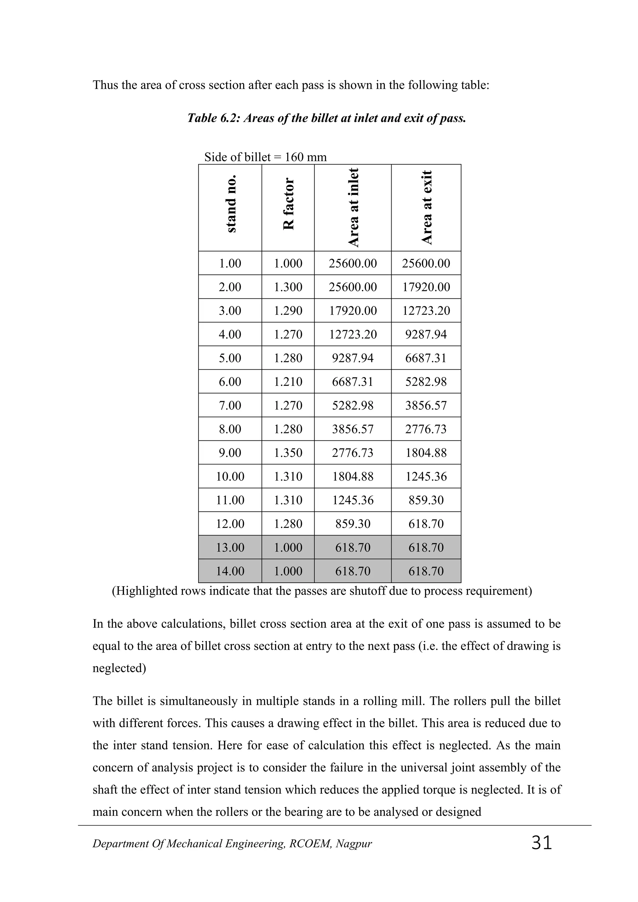
![Thus the area of the billet at the entry to the stand no 9 i.e. A1 = 2776.73 mm2
The area of cross section at the exit of stand no 9 is A2 = 1804.88 mm2
As the billet passes through the stands its cross section after passing from each stand
differs from the shape with which it feeds into the rollers i.e. for a particular stand if the
exit cross section is circular for the next stand the inlet cross section becomes elliptical
which means that if the inlet section is circular the exit section should be elliptical and
vice versa. [10]
Thus the diameters of the billet at the inlet and exit section are calculated as follows
Diameter of billet at the inlet D1 =�2776.73 × 4 ×
1
𝜋
= 59.46 mm
Similarly, diameter at the exit: D2 = 47.94 mm (for perfectly circular shape)
But, since the section at exit is not completely circular and is elliptical due to roll
geometry,
1804.88 = 𝜋 × ℎR
2× Rw2
Where, h2 = 17.67 mm, which is found from the roll geometry and roll gap given
∴ 𝑤2 = 32.6 𝑚𝑚
Figure 6.1: incoming and outgoing section geometry of work piece at roll pass.(a):circle
to oval, (b): oval to circle
Department Of Mechanical Engineering, RCOEM, Nagpur 32](https://image.slidesharecdn.com/projectreport-140702000203-phpapp02/75/DESIGN-ANALYSIS-OF-UNIVERSAL-JOINT-SHAFT-FOR-ROLLING-MILLS-41-2048.jpg)
![CHAPTER 07 ANALYSIS FOR CALCULATION OF ROLL
FORCE AND TORQUE
7.1 Contact length or the roll bite length:
It is the distance between the two points on the rolls, along the circumference at which the
work piece enters and leaves the rollers. In this case,
𝐿 𝑟 = �2𝑅𝑖(ℎ1−ℎ2)
𝑅𝑖 = Inner roll radius =
360.5−2∗12.72
2
= 167.53𝑚𝑚
By substituting 𝑅𝑖,ℎ𝑖 = 29.73𝑚𝑚 , ℎ2 = 32.6𝑚𝑚, 𝐿 𝑟= 63.56mm
For the equivalent rectangle assumption, the section height 2h at any distance x from the
entry is given by
ℎ = ℎ1 −
𝐿 𝑟
𝑅𝑖
𝑥 +
𝑥2
2𝑅𝑖
ℎ = 29.73 −
63.56
167.53
𝑥 +
𝑥2
2 ∗ 167.53
ℎ = 29.73 − 0.3974𝑥 + 2.984 × 10⁻³
𝑥2
(7.1)
The section maximum width 2𝑤 is approximated to have a parabolic distribution along
the roll bite length, given by
𝑤 = 𝑤1 − 2(𝑤1-𝑤2)
𝑥
𝐿 𝑟
+ (𝑤1 − 𝑤2)
𝑥2
𝐿 𝑟
2
𝑤 = 𝑤1 − 2(29.73 − 32.67)
𝑥
63.56
+
(29.73 − 32.67)
63.562
𝑥2
𝑤 = 29.73 − 0.0925𝑥 − 7.297 × 10⁻⁴
𝑥2
(7.2)
Equation 7.2 is formed such that it satisfies the boundary conditions 𝑤 = 𝑤1at 𝑥 = 0 and
𝑤 = 𝑤2 at 𝑥 = 𝑙 𝑟 𝑎𝑛𝑑
𝑑𝑤
𝑑𝑥
= 0 at 𝑥 = 𝑙 𝑟 which are the conditions taken by default
while analyzing or formulating the rolling process for sheet rolling. [10]
The projected area of work piece-roll contact surface on the x-z plane is approximated to a
semi elliptic shape of a width 2b at exit and 2b at any section at distance x from the entry
expressed as
𝑏 = 𝑏2�
2𝑥
𝐿 𝑟
−
𝑥2
𝐿 𝑟
Department Of Mechanical Engineering, RCOEM, Nagpur 34](https://image.slidesharecdn.com/projectreport-140702000203-phpapp02/75/DESIGN-ANALYSIS-OF-UNIVERSAL-JOINT-SHAFT-FOR-ROLLING-MILLS-43-2048.jpg)
![𝑏 =
26.72
2
�
2𝑥
63.56
−
𝑥2
63.562
(7.3)
7.2 Calculation of effective roll radius
The effective roll radius is obtained from the maximum roll radius, 𝑅 𝑜 , roll gap G and
work piece exit maximum width 2𝑤2 and exit cross section area 𝐴2 as,
𝑅 𝑒 = 𝑅 𝑜 − 0.5 �
𝐴2
2𝑤2
− 𝐺� (7.4)
𝑅 𝑒 = 180.25 − 0.5 �
1804.88
2 ∗ 17.67
− 11.5�
𝑅 𝑒 = 164.125𝑚𝑚
The above equation 9.4 works only when the exit cross sectional shape is rectangular.
Equation 9.4 is based on equivalent rectangular approximation method that transfer the
non-rectangular cross section into rectilinear one of width equal to the maximum width of
the cross section while the net cross sectional area is maintained the same. [10]
7.3 Calculation of strain and strain rate
For homogeneous deformation of work piece in the direction of height and width, the
respective strain component can be found as follows.
The load deflection curve for ductile material is shown in the following figure.
Hot rolling involves plastic deflection of the work piece strain =
𝑐ℎ𝑎𝑛𝑔𝑒 𝑖𝑛 𝑙𝑒𝑛𝑔𝑡ℎ
𝑜𝑟𝑖𝑔𝑖𝑛𝑎𝑙 𝑙𝑒𝑛𝑔𝑡ℎ
Figure 9.1: Stress strain relation for steels
Department Of Mechanical Engineering, RCOEM, Nagpur 35](https://image.slidesharecdn.com/projectreport-140702000203-phpapp02/75/DESIGN-ANALYSIS-OF-UNIVERSAL-JOINT-SHAFT-FOR-ROLLING-MILLS-44-2048.jpg)
![𝑑𝜀 = −
𝑑𝑥
𝑥
=
𝑓𝑖𝑛𝑎𝑙 𝑙𝑒𝑛𝑔𝑡ℎ − 𝑖𝑛𝑖𝑡𝑖𝑎𝑙 𝑙𝑒𝑛𝑔𝑡ℎ
𝑜𝑟𝑖𝑔𝑖𝑛𝑎𝑙 𝑙𝑒𝑛𝑔𝑡ℎ
Integrating, with limit from 𝐿𝑖 𝑡𝑜𝐿 𝑜
𝟄 = � 𝑑𝟄 = �
𝑑𝑥
𝑥
𝐿0
𝐿 𝑖
= [ln 𝑥]
= − ln �
𝑙 𝑖
𝑙 𝑜
� (7.5)
Note: the ‘- ve ‘sign can be neglected for calculations as it indicates whether strain is due
to tension or compression.
Thus along the height of the work piece,
𝟄 𝑦 = ln �
ℎ
ℎ1
�
𝟄 𝑦 = ln
29.73
17.67
= 0.52
Similarly, strain along the width direction,
𝟄 𝑧 = ln �
𝑤1
𝑤2
�
𝟄 𝑧 =
17.6
29.73
= −0.0943
The volume of the work piece remains constant during the complete rolling process.
Thus,
𝟄 𝑥 + 𝟄 𝑦 + 𝟄 𝑧 = 0
𝟄 𝑥 = −�𝟄 𝑦 + 𝟄 𝑧�
𝟄 𝑥 = −(0.52 − 0.0943) = −0.4257
Neglecting the shear strain components, the effective strain obtained as
Department Of Mechanical Engineering, RCOEM, Nagpur 36](https://image.slidesharecdn.com/projectreport-140702000203-phpapp02/75/DESIGN-ANALYSIS-OF-UNIVERSAL-JOINT-SHAFT-FOR-ROLLING-MILLS-45-2048.jpg)
![𝟄 𝑟���=�
2
3
�𝟄 𝑥
2 + 𝟄 𝑦
2 + 𝟄 𝑧
2� (7.6)
𝟄 𝑟��� = 0.5541
7.4 Calculation of effective strain rate
Strain rate or the effective strain rate is the rate of change of strain, and is given by
𝜀̅̇ =
𝜀
𝑡 𝑝
(7.7)
Where 𝜀 is the strain and 𝑡 𝑝 is the time required for a paint or the work piece to pass
through contact length. [11]
𝑡 𝑝 Can be calculated by the relation
𝑡 𝑝 =
60× 𝐿 𝑟
2𝜋𝑁 𝑅 𝑒𝑓𝑓
(7.8)
𝑡 𝑝 =
60 ∗ 63.56
2𝜋 ∗ 79 ∗ �
167.53+180.25
2
�
𝑡𝑝 = 0.047𝑠𝑒𝑐
Thus, the strain rates can be calculated by using equation (7.8) as,
𝜀̇ 𝑦 =
𝜀
𝑡 𝑝
=
0.52
0.047
= 11.108 s-1
𝜀̇𝑧 =
𝜀 𝑧
𝑡 𝑝
=
−0.0943
0.047
𝜀̇𝑧 = −2.014 s-1
Again, by law of conservation of volume,
𝜖 𝑥̇ =−�𝜖 𝑦̇ + 𝜖 𝑧̇ � (7.9)
𝜖 𝑥̇ = 0.094 s-1
Resultant strain rate,
Department Of Mechanical Engineering, RCOEM, Nagpur 37](https://image.slidesharecdn.com/projectreport-140702000203-phpapp02/75/DESIGN-ANALYSIS-OF-UNIVERSAL-JOINT-SHAFT-FOR-ROLLING-MILLS-46-2048.jpg)
![𝜎𝑡 = 0.28 ∗ 𝑞( 𝑐, 𝑡)exp �
𝑐 + 0.32
0.19 (𝑐 + 0.41)
−
0.01
𝑐 + 0.05
�
𝑞(𝑐, 𝑡) = 30(𝑐 + 0.9)(𝑇 − 0.95 ∗
𝑐 + 0.49
𝑐 + 0.42
)
𝑓𝑟 = �
𝜀̇
10
�
𝑚
. �
𝜀̇
100
�
𝑚
2.4
. (
𝜀̇
1000
) 𝑚/15
𝑚 = (0.081𝐶 − 0.154)𝑇 − 0.019𝐶 + .207 +
0.027
𝐶+0.32
From the above values and graph we can conclude that the flow stresses for different steels
with different carbon percentages are nearly the same at the rolling conditions. [6]
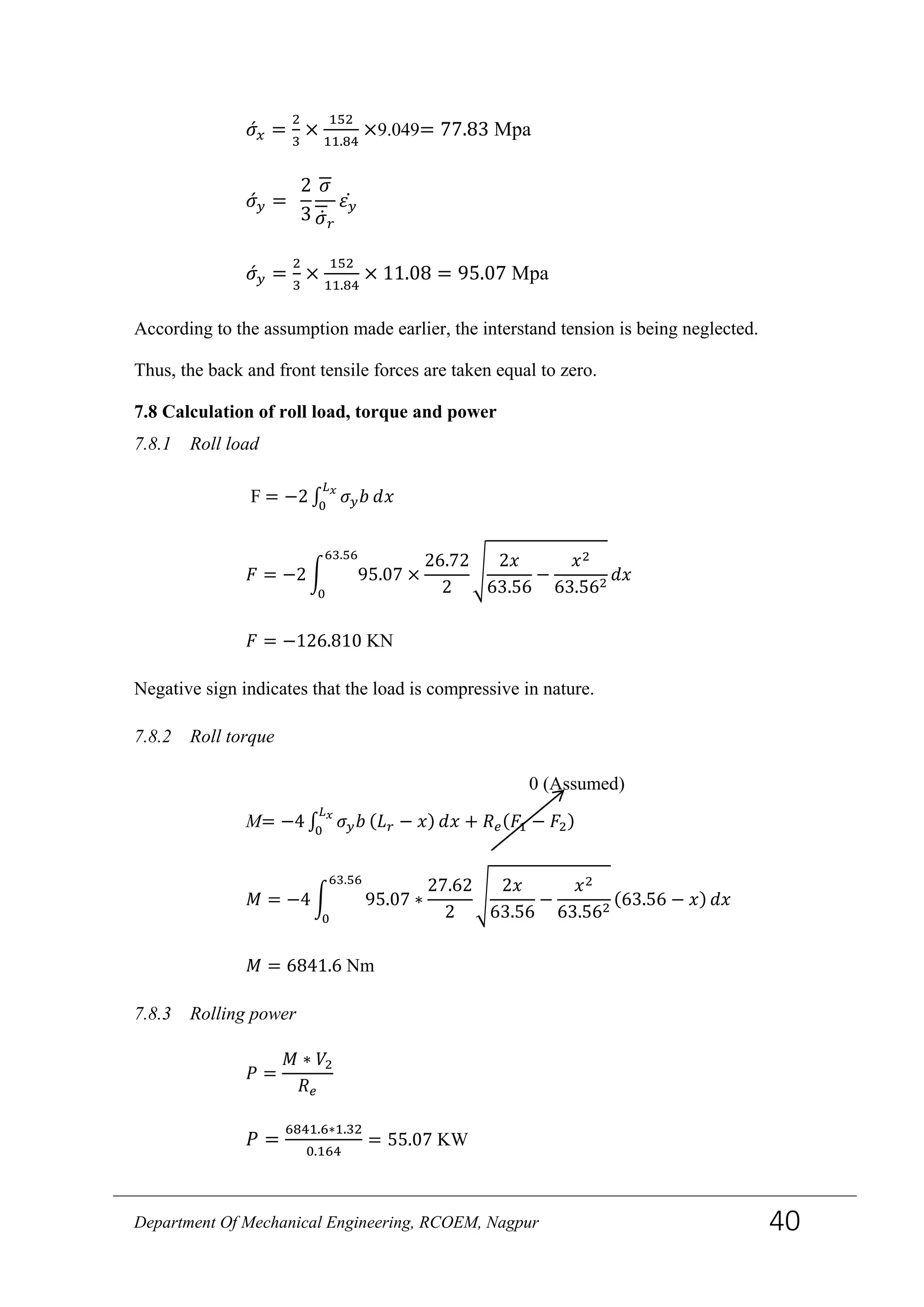
Thus, considering the mean value of flow stress as 152Mpa, the deviatoric stress
components can be found out.
7.7 Calculation of deviatoric stress components
The deviatoric stress components are those which need to be exceeded at a given
conditions for changing the cross section of the work piece.
These components in the 3 directions x, y and z can be found by levy-mises flow rule
𝜎́ 𝑥 =
2
3
𝜎
𝜎̇ 𝑟
𝜀 𝑥̇
Figure 9.2: Temperature flow stress relation for steels at given strain rate
Department Of Mechanical Engineering, RCOEM, Nagpur 39](https://image.slidesharecdn.com/projectreport-140702000203-phpapp02/75/DESIGN-ANALYSIS-OF-UNIVERSAL-JOINT-SHAFT-FOR-ROLLING-MILLS-48-2048.jpg)


![superposition of a number of SDOF characteristics (when the system is linear time-
invariant).
11.4 Multi Degree Of Freedom:
Multiple degree-of-freedom (MDOF) systems are described by the following equation:
Mẍ(t) + Cẋ(t) +Kx(t) = f(t)
The transfer function H(s) between displacement and force, X (s) = H(s)F(s) , is given by,
𝐻(𝑠) = [𝑀𝑠2
+ 𝐶𝑠 + 𝐾]−1
=
𝑁(𝑠)
𝑑(𝑠)
Where, N(s) = adj(Ms2 + Cs + K)
And, d(s) = det(Ms2 + Cs + K)
When the damping is small, the roots of the characteristic polynomial d(s) are complex
conjugate pole pairs, 𝜆 𝑚and𝜆 𝑚∗, m = 1…..N m, with Nmthe number of modes of the
system. The transfer function can be rewritten in a pole-residue form which is said to be
the “modal” model.
𝐻( 𝑠) = ∑
𝑅 𝑚
𝑠−𝜆 𝑚
𝑁 𝑚
𝑚=1 +
𝑅 𝑚∗
𝑠−𝜆 𝑚∗
The residue matrices Rm, m =1……Nm, are defined by, 𝑅 𝑚 = lim 𝑠→𝜆 𝑚
𝐻(𝑠)(𝑠 − 𝜆 𝑚)
It can be shown that the matrix R mis of rank one meaning that R mcan be decomposed
as,
Figure 11.3: MDOF system
Department Of Mechanical Engineering, RCOEM, Nagpur 56](https://image.slidesharecdn.com/projectreport-140702000203-phpapp02/75/DESIGN-ANALYSIS-OF-UNIVERSAL-JOINT-SHAFT-FOR-ROLLING-MILLS-65-2048.jpg)
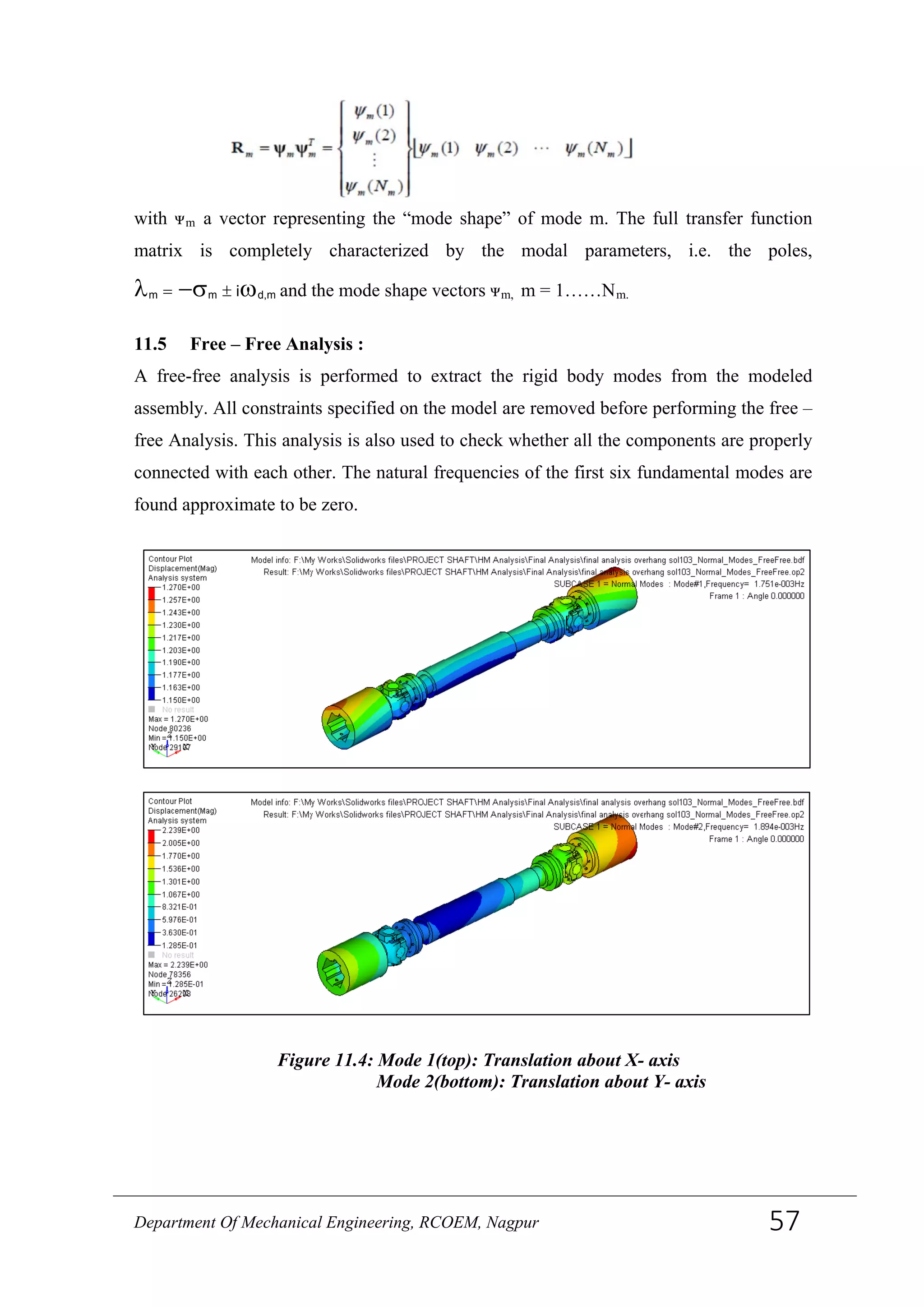


This project report presents a design analysis of a universal joint shaft for rolling mills, submitted by a group of mechanical engineering students at Shri Ramdeobaba College of Engineering & Management during the 2013-2014 academic year. It discusses the structure, advantages, and applications of universal joints, supported by a literature review on their historical development and mathematical analysis. The document includes chapters detailing the project methodology, validation of results, and future scope, alongside acknowledgments for instructional and technical support.


