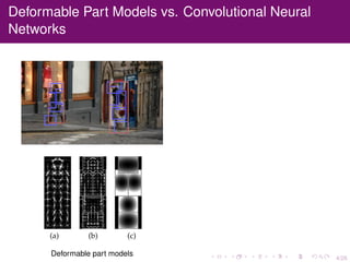
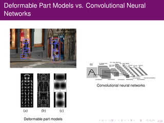
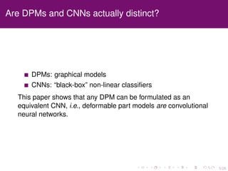
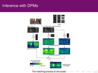
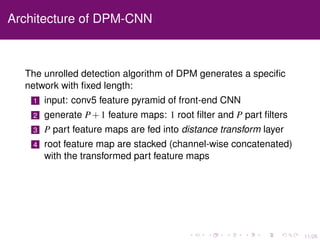
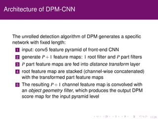
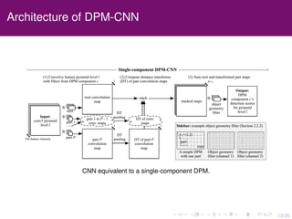
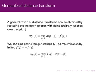
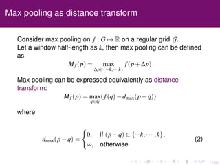
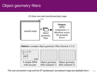
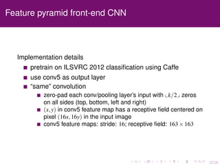
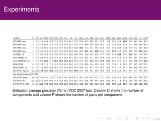
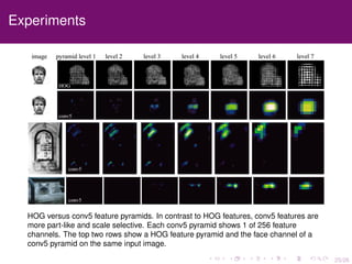
The document discusses the equivalence of deformable part models (DPMs) and convolutional neural networks (CNNs), presenting a framework to construct a CNN from any DPM. It describes the architecture of a DPM-CNN that combines features from both models and details various implementation strategies and experiments. The paper highlights performance improvements using DPM-CNNs over traditional feature extraction methods.

1. 1/26
Deformable Part Models are Convolutional
Neural Networks
Ross Girshick, Forrest Iandola, Trevor Darrell, Jitendra Malik
Presentor: YANG Wei
January 25, 2016

2. 2/26
Outline
1 Introduction
2 DeepPyramid DPMs
Feature pyramid front-end CNN
Constructing an equivalent CNN from a DPM
3 Implementation details
4 Experiments

3. 3/26
Outline
1 Introduction
2 DeepPyramid DPMs
Feature pyramid front-end CNN
Constructing an equivalent CNN from a DPM
3 Implementation details
4 Experiments

4. 4/26
Deformable Part Models vs. Convolutional Neural
Networks
Deformable part models

5. 4/26
Deformable Part Models vs. Convolutional Neural
Networks
Deformable part models
Convolutional neural networks

6. 5/26
Are DPMs and CNNs actually distinct?
DPMs: graphical models
CNNs: “black-box” non-linear classifiers
This paper shows that any DPM can be formulated as an
equivalent CNN, i.e., deformable part models are convolutional
neural networks.

7. 6/26
Outline
1 Introduction
2 DeepPyramid DPMs
Feature pyramid front-end CNN
Constructing an equivalent CNN from a DPM
3 Implementation details
4 Experiments

8. 7/26
DeepPyramid DPMs
Schematic model overview: “front-end CNN” + DPM-CNN
input: image pyramid
output: object detection scores

9. 8/26
Feature pyramid front-end CNN
front-end CNN: AlexNet (conv1-conv5).
A CNN that maps an image pyramid to a feature pyramid
AlexNet
single-scale architecture

10. 9/26
Constructing an equivalent CNN from a DPM
A single-component DPM.
mixture of components
component = root filter + part filter

11. 10/26
Inference with DPMs
The matching process at one scale.

12. 11/26
Architecture of DPM-CNN
The unrolled detection algorithm of DPM generates a specific
network with fixed length:
1 input: conv5 feature pyramid of front-end CNN

13. 11/26
Architecture of DPM-CNN
The unrolled detection algorithm of DPM generates a specific
network with fixed length:
1 input: conv5 feature pyramid of front-end CNN
2 generate P+1 feature maps: 1 root filter and P part filters

14. 11/26
Architecture of DPM-CNN
The unrolled detection algorithm of DPM generates a specific
network with fixed length:
1 input: conv5 feature pyramid of front-end CNN
2 generate P+1 feature maps: 1 root filter and P part filters
3 P part feature maps are fed into distance transform layer

15. 11/26
Architecture of DPM-CNN
The unrolled detection algorithm of DPM generates a specific
network with fixed length:
1 input: conv5 feature pyramid of front-end CNN
2 generate P+1 feature maps: 1 root filter and P part filters
3 P part feature maps are fed into distance transform layer
4 root feature map are stacked (channel-wise concatenated)
with the transformed part feature maps

16. 11/26
Architecture of DPM-CNN
The unrolled detection algorithm of DPM generates a specific
network with fixed length:
1 input: conv5 feature pyramid of front-end CNN
2 generate P+1 feature maps: 1 root filter and P part filters
3 P part feature maps are fed into distance transform layer
4 root feature map are stacked (channel-wise concatenated)
with the transformed part feature maps
5 The resulting P+1 channel feature map is convolved with
an object geometry filter, which produces the output DPM
score map for the input pyramid level

17. 12/26
Architecture of DPM-CNN
CNN equivalent to a single-component DPM.

18. 13/26
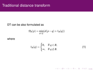
Traditional distance transform
Traditional distance transforms are defined for sets of points on
a grid [FH05].
G: grid
d(p−q): measure of
distance between points
p,q ∈ G
B ⊆ G
Then the distance transform of
B on G
DB(p) = min
q∈B
d(p−q)
Distance transform (Euclidean distance)

19. 14/26
Traditional distance transform
DT can be also formulated as
DB(p) = min
q∈G
(d(p−q)+1B(q))
where
1B(q) =
0, if q ∈ B,
∞, if q /∈ B.
(1)

20. 15/26
Generalized distance transform
A generalization of distance transforms can be obtained by
replacing the indicator function with some arbitrary function
over the grid G
Df (p) = min
q∈G
(d(p−q)+ f (q))
We can also define the generalized DT as maximization by
letting f(q) = −f (q)
Df (p) = max
q∈G
(f(q)−d(p−q))

21. 16/26
Distance transform in DPM
In DPM, after computing filter responses we transform the
responses of the part filters to allow spatial uncertainty,
Di(x,y) = max
dx,dy
(Ri(x+dx,y+dy)−wi ·φd(dx,dy))
where
φd(dx,dy) = [dx,dy,dx2
,,dy2
]
The value Di(x,y) is the maximum contribution of the part
to the score of a root location that places the anchor of this
part at position (x,y).

22. 16/26
Distance transform in DPM
In DPM, after computing filter responses we transform the
responses of the part filters to allow spatial uncertainty,
Di(x,y) = max
dx,dy
(Ri(x+dx,y+dy)−wi ·φd(dx,dy))
where
φd(dx,dy) = [dx,dy,dx2
,,dy2
]
The value Di(x,y) is the maximum contribution of the part
to the score of a root location that places the anchor of this
part at position (x,y).
By letting p = (x,y), p−q = (dx,dy) and
d(p−q) = w·φ(p−q), we can see that it is exactly in the
form of distance transform.

23. 17/26
Max pooling as distance transform
Consider max pooling on f : G → R on a regular grid G.
Let a window half-length as k, then max pooling can be defined
as
Mf (p) = max
∆p∈{−k,···,k}
f(p+∆p)
Max pooling can be expressed equivalently as distance
transform:
Mf (p) = max
q∈G
(f(q)−dmax(p−q))
where
dmax(p−q) =
0, if (p−q) ∈ {−k,··· ,k},
∞, otherwise .
(2)

24. 18/26
Generalize max pooling to distance transform pooling
We can generalize max pooling to distance transform pooling:
unlike max pooling, the distance transform of f at p is
taken over the entire domain G
rather than specifying a fixed pooling window a priori, the
shape of the pooling region can be learned from the data.

25. 18/26
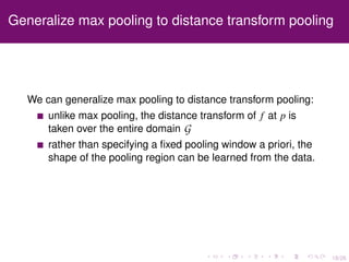
Generalize max pooling to distance transform pooling
We can generalize max pooling to distance transform pooling:
unlike max pooling, the distance transform of f at p is
taken over the entire domain G
rather than specifying a fixed pooling window a priori, the
shape of the pooling region can be learned from the data.
The released code does not include the DT pooling layer.
Please refer to [OW13] for more details.

26. 19/26
Object geometry filters
The root convolution map and the DT pooled part convolution maps are stacked into a

27. 20/26
Combining mixture components with maxout
CNN equivalent to a multi-component DPM. A multi-component DPM-CNN is
composed of one DPM-CNN per component and a maxout [GWFM+13] layer that
takes a max over component DPM-CNN outputs at each location.

28. 21/26
Outline
1 Introduction
2 DeepPyramid DPMs
Feature pyramid front-end CNN
Constructing an equivalent CNN from a DPM
3 Implementation details
4 Experiments

29. 22/26
Feature pyramid front-end CNN
Implementation details
pretrain on ILSVRC 2012 classification using Caffe
use conv5 as output layer
“same” convolution
zero-pad each conv/pooling layer’s input with k/2 zeros
on all sides (top, bottom, left and right)
(x,y) in conv5 feature map has a receptive field centered on
pixel (16x,16y) in the input image
conv5 feature maps: stride: 16; receptive field: 163×163

30. 23/26
Outline
1 Introduction
2 DeepPyramid DPMs
Feature pyramid front-end CNN
Constructing an equivalent CNN from a DPM
3 Implementation details
4 Experiments

31. 24/26
Experiments
Detection average precision (%) on VOC 2007 test. Column C shows the number of
components and column P shows the number of parts per component.

32. 25/26
Experiments
HOG versus conv5 feature pyramids. In contrast to HOG features, conv5 features are
more part-like and scale selective. Each conv5 pyramid shows 1 of 256 feature
channels. The top two rows show a HOG feature pyramid and the face channel of a
conv5 pyramid on the same input image.

33. 26/26
References
Pedro F Felzenszwalb and Daniel P Huttenlocher, Pictorial structures for object
recognition, International Journal of Computer Vision 61 (2005), no. 1, 55–79.
Ian J Goodfellow, David Warde-Farley, Mehdi Mirza, Aaron Courville, and Yoshua
Bengio, Maxout networks, arXiv preprint arXiv:1302.4389 (2013).
Wanli Ouyang and Xiaogang Wang, Joint deep learning for pedestrian detection,
ICCV, IEEE, 2013, pp. 2056–2063.