Downloaded 54 times
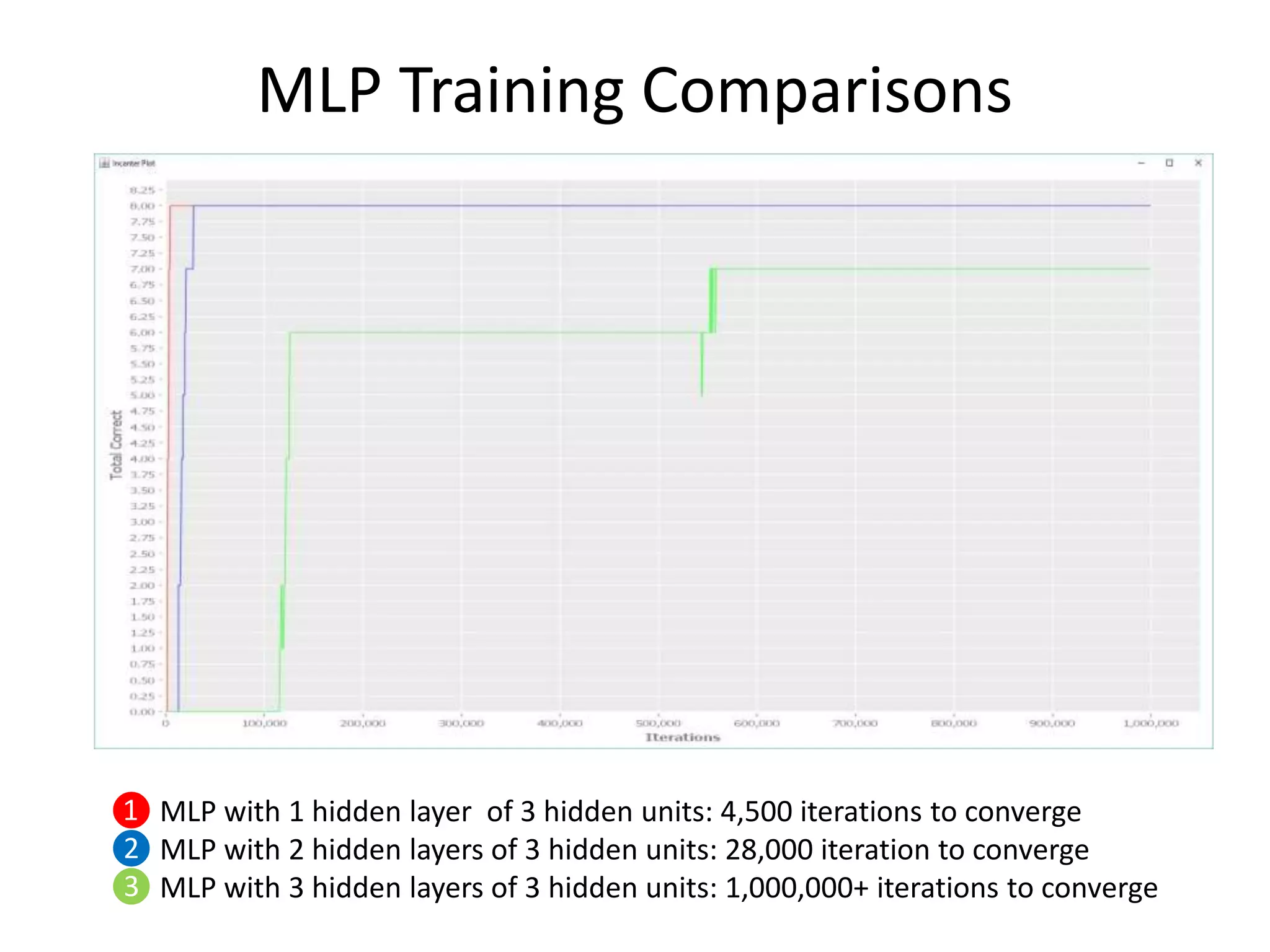
![Identity Function Example
• Tom Mitchell, Machine Learning, Chpt 4., 1st edition.
(def if-td
[[[1 0 0 0 0 0 0 0] [1 0 0 0 0 0 0 0]]
[[0 1 0 0 0 0 0 0] [0 1 0 0 0 0 0 0]]
[[0 0 1 0 0 0 0 0] [0 0 1 0 0 0 0 0]]
[[0 0 0 1 0 0 0 0] [0 0 0 1 0 0 0 0]]
[[0 0 0 0 1 0 0 0] [0 0 0 0 1 0 0 0]]
[[0 0 0 0 0 1 0 0] [0 0 0 0 0 1 0 0]]
[[0 0 0 0 0 0 1 0] [0 0 0 0 0 0 1 0]]
[[0 0 0 0 0 0 0 1] [0 0 0 0 0 0 0 1]]])
• Ran 3 examples of MLPs on Identity function.
– A 1 hidden layer MLP: 8 x 3 x 8
– A 2 hidden layer MLP: 8 x 3 x 3 x 8
– A 3 hidden layer MLP: 8 x 3 x 3 x 3 x 8](https://image.slidesharecdn.com/deep-learning-lispnyc-june-2017-170625181139/75/Deep-Learning-11-2048.jpg)
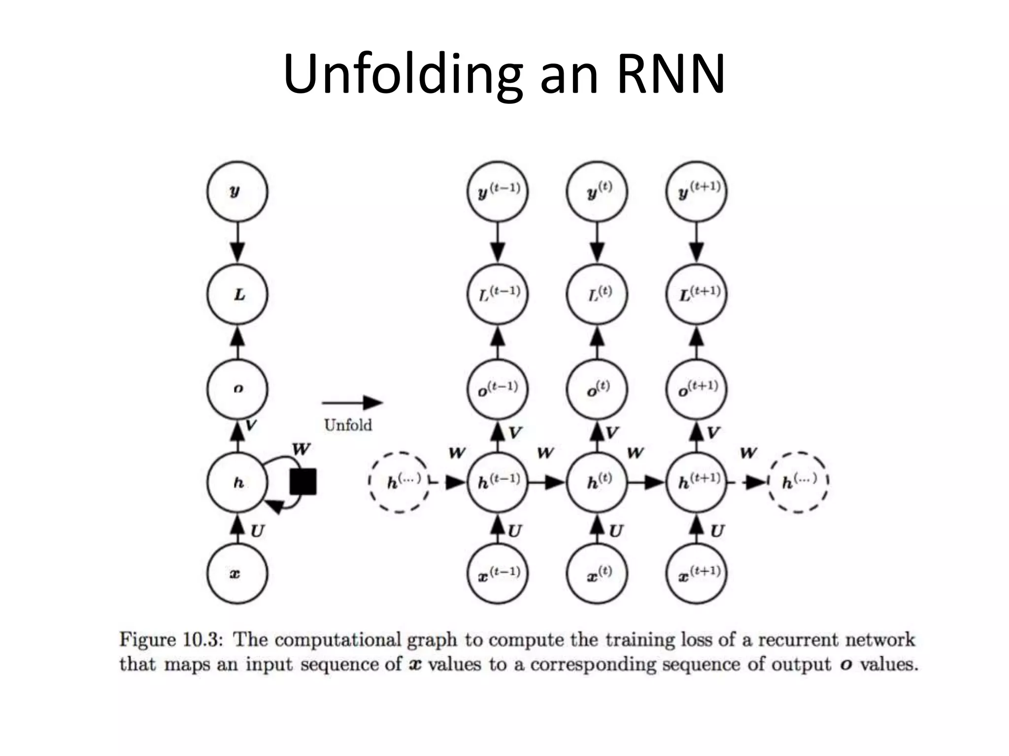
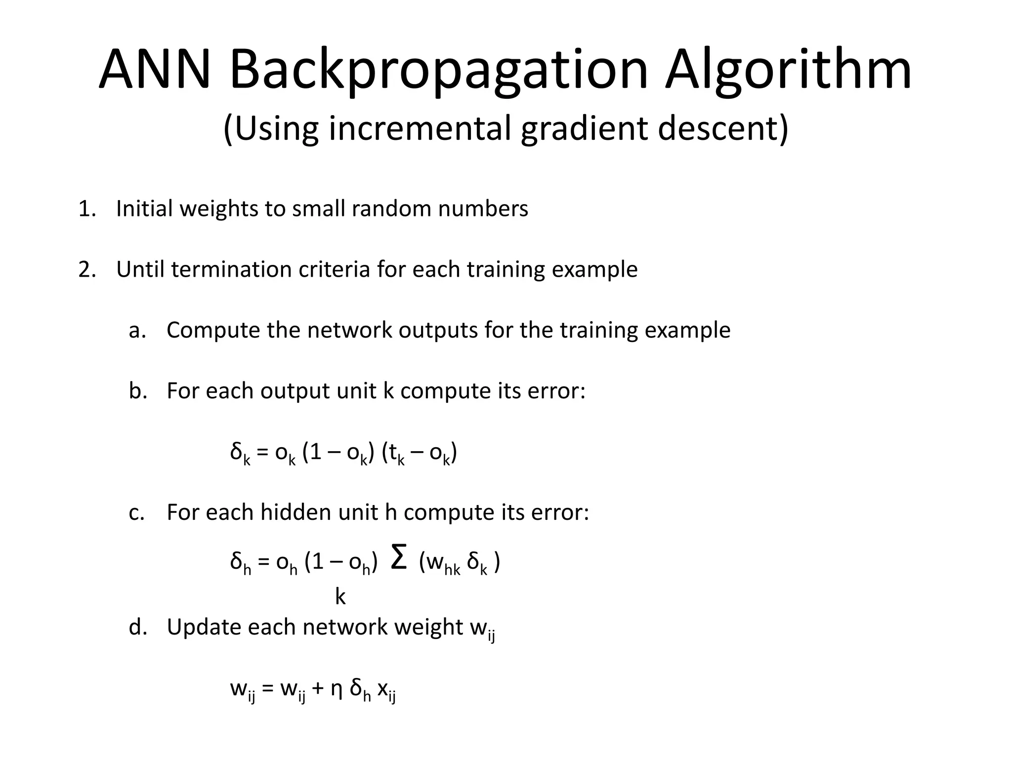
![Training RNNs
• Backpropagation in Computational Graphs
– Backprogation can be derived for any computational graph by recursively applying the chain
rule. (Deep Learning, Chapter 6)
– The backprogation algorithm consists of performing a Jacobian-gradient-product for each
operation in the graph
– In vector calculus, the Jacobian matrix is the matrix of all first-order partial derivatives of a
vector-valued function
• Backpropagation Through Time (BPTT).
– Gradient at each output depends not only on the calculations of the current time step, but
also the previous time steps.
– Vanilla RNNs trained with BPTT have difficulties learning long-term dependencies, i.e.
dependencies between (words) steps that are far apart)
• “I grew up in France… I speak fluent French”
– Suffers from vanishing/exploding gradient problem.
• Vanishing gradient: your gradients get smaller and smaller in magnitude as you backpropagate through earlier
layers (or through time).
• Activation functions like the sigmoid function produce gradients in range [-1,1] which easily causes the gradient
to vanish in earlier layers.
• Exploding gradient: more of an issue with recurrent networks, where the opposite happens due to a Jacobian
with determinant greater than 1.
– Certain types of RNNs (like LSTMs) were specifically designed to get around these problems.](https://image.slidesharecdn.com/deep-learning-lispnyc-june-2017-170625181139/75/Deep-Learning-41-2048.jpg)


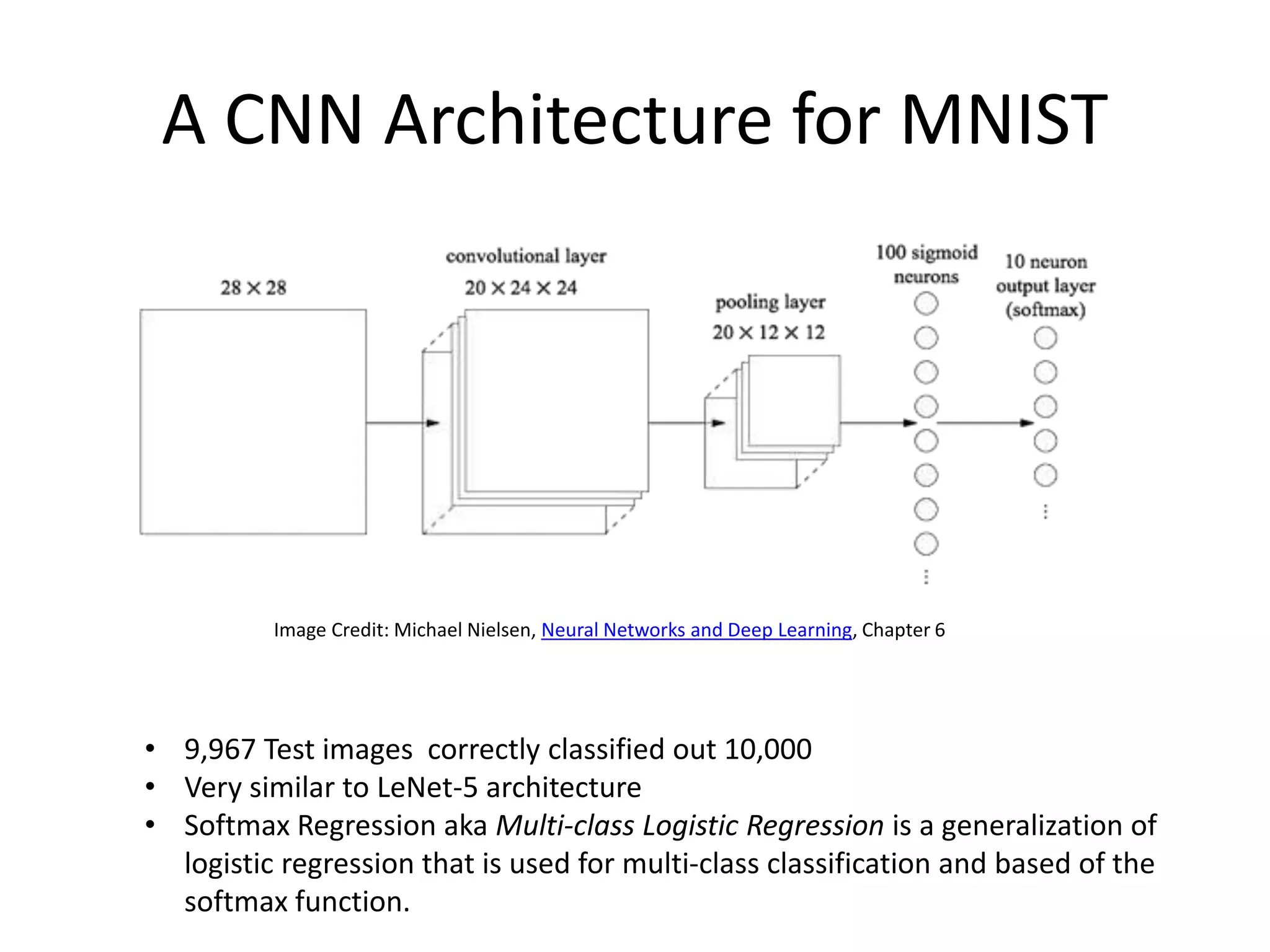
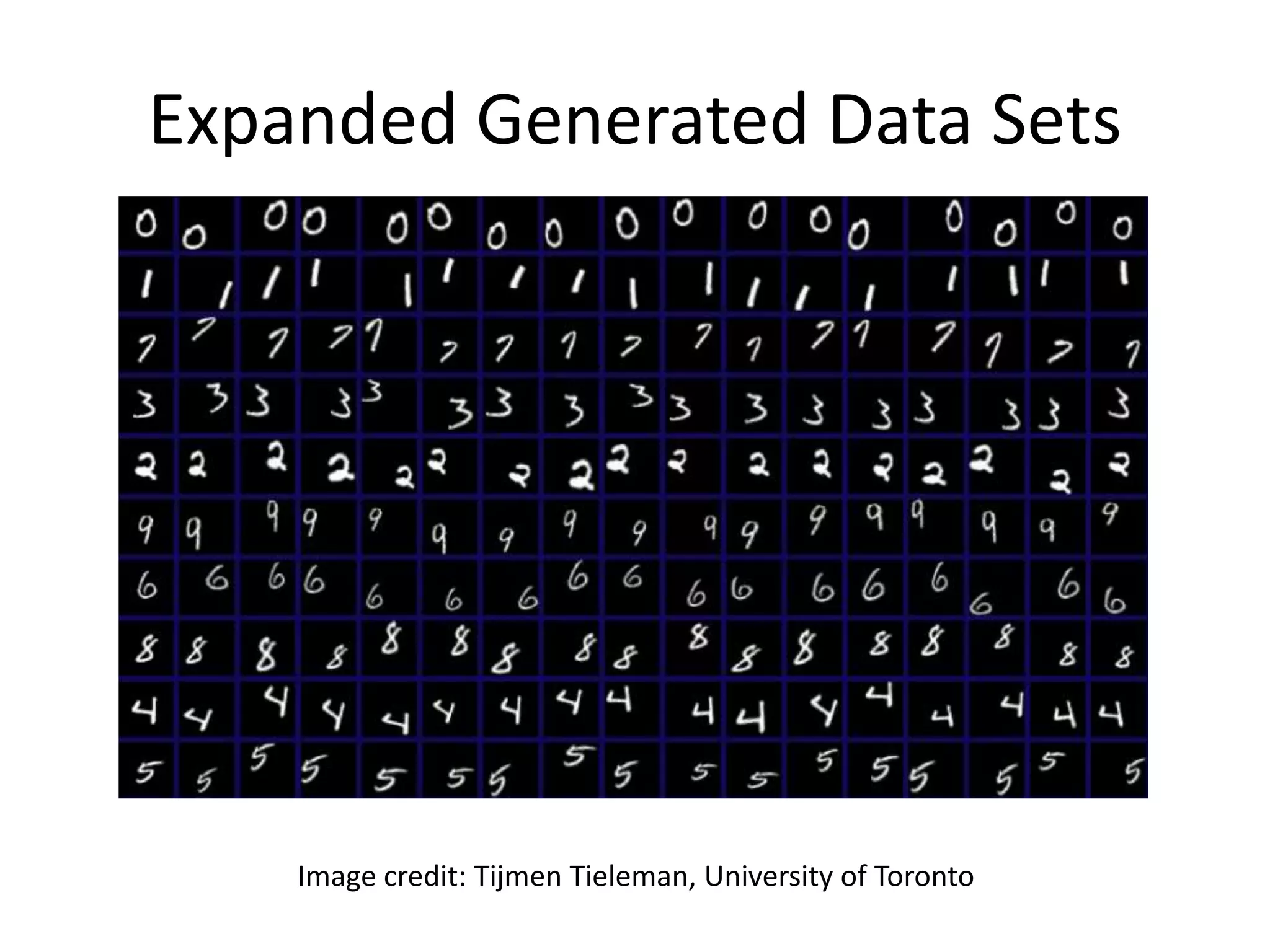
The document provides an overview of deep learning, focusing on key topics such as convolutional neural networks (CNNs) and recurrent neural networks (RNNs). CNNs are biologically-inspired networks designed for processing image data, while RNNs are suited for sequential data, allowing for information flow in both directions. The text also discusses various training techniques, architectures, and applications, highlighting advancements in the field.


![Coded Agents – with UiPath SDK + LangGraph [Virtual Hands-on Workshop]](https://cdn.slidesharecdn.com/ss_thumbnails/codedagentsdeck-251215155422-5497c599-thumbnail.jpg?width=640&height=640&fit=bounds)


