Introduction to Deep Learning
BayPiggies Meetup 08/23/2018
LinkedIn Sunnyvale
Unify Meeting Room
Oswald Campesato
ocampesato@yahoo.com
Highlights/Overview
ļ‚“intro to AI/ML/DL/NNs
ļ‚“Hidden layers
ļ‚“Initialization values
ļ‚“Neurons per layer
ļ‚“Activation function
ļ‚“cost function
ļ‚“gradient descent
ļ‚“learning rate
ļ‚“Dropout rate
ļ‚“what are CNNs
The Data/AI Landscape
Use Cases for Deep Learning
ļ‚“computer vision
ļ‚“speech recognition
ļ‚“image processing
ļ‚“bioinformatics
ļ‚“social network filtering
ļ‚“drug design
ļ‚“Recommendation systems
ļ‚“Bioinformatics
ļ‚“Mobile Advertising
ļ‚“Many others
NN 3 Hidden Layers: Classifier
NN: 2 Hidden Layers (Regression)
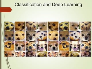
Classification and Deep Learning
A Basic Model in Machine Learning
ļ‚“Let’s perform the following steps:
ļ‚“1) Start with a simple model (2 variables)
ļ‚“2) Generalize that model (n variables)
ļ‚“3) See how it might apply to a NN
Linear Regression
ļ‚“One of the simplest models in ML
ļ‚“Fits a line (y = m*x + b) to data in 2D
ļ‚“Finds best line by minimizing MSE:
m = slope of the best-fitting line
b = y-intercept of the best-fitting line
Linear Regression in 2D: example
Sample Cost Function #1 (MSE)
Linear Regression: example #1
ļ‚“One feature (independent variable):
X = number of square feet
ļ‚“Predicted value (dependent variable):
Y = cost of a house
ļ‚“A very ā€œcoarse grainedā€ model
ļ‚“We can devise a much better model
Linear Regression: example #2
ļ‚“Multiple features:
ļ‚“X1 = # of square feet
ļ‚“X2 = # of bedrooms
ļ‚“X3 = # of bathrooms (dependency?)
ļ‚“X4 = age of house
ļ‚“X5 = cost of nearby houses
ļ‚“X6 = corner lot (or not): Boolean
ļ‚“a much better model (6 features)
Linear Multivariate Analysis
ļ‚“General form of multivariate equation:
ļ‚“Y = w1*x1 + w2*x2 + . . . + wn*xn + b
ļ‚“w1, w2, . . . , wn are numeric values
ļ‚“x1, x2, . . . , xn are variables (features)
ļ‚“Properties of variables:
Can be independent (NaĆÆve Bayes)
weak/strong dependencies can exist
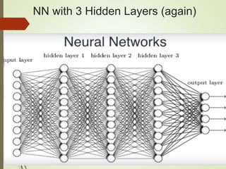
NN with 3 Hidden Layers (again)
Neural Networks: equations
ļ‚“Node ā€œvaluesā€ in first hidden layer:
ļ‚“N1 = w11*x1+w21*x2+…+wn1*xn
ļ‚“N2 = w12*x1+w22*x2+…+wn2*xn
ļ‚“N3 = w13*x1+w23*x2+…+wn3*xn
ļ‚“. . .
ļ‚“Nn = w1n*x1+w2n*x2+…+wnn*xn
ļ‚“Similar equations for other pairs of layers
Neural Networks: Matrices
ļ‚“From inputs to first hidden layer:
Y1 = W1*X + B1 (X/Y1/B1: vectors; W1: matrix)
From first to second hidden layers:
Y2 = W2*X + B2 (X/Y2/B2: vectors; W2: matrix)
From second to third hidden layers:
Y3 = W3*X + B3 (X/Y3/B3: vectors; W3: matrix)
 Apply an ā€œactivation functionā€ to y values
Neural Networks (general)
ļ‚“Multiple hidden layers:
Layer composition is your decision
ļ‚“Activation functions: sigmoid, tanh, RELU
https://en.wikipedia.org/wiki/Activation_function
ļ‚“Back propagation (1980s)
https://en.wikipedia.org/wiki/Backpropagation
ļ‚“=> Initial weights: small random numbers
Euler’s Function (e: 2.71828. . .)
The sigmoid Activation Function
The tanh Activation Function
The ReLU Activation Function
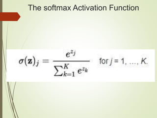
The softmax Activation Function
Activation Functions in Python
ļ‚“import numpy as np
ļ‚“...
ļ‚“# Python sigmoid example:
ļ‚“z = 1/(1 + np.exp(-np.dot(W, x)))
ļ‚“...
ļ‚“# Python tanh example:
ļ‚“z = np.tanh(np.dot(W,x));
ļ‚“# Python ReLU example:
ļ‚“z = np.maximum(0, np.dot(W, x))
What’s the ā€œBestā€ Activation Function?
ļ‚“Initially: sigmoid was popular
ļ‚“Then: tanh became popular
ļ‚“Now: RELU is preferred (better results)
ļ‚“Softmax: for FC (fully connected) layers
ļ‚“NB: sigmoid and tanh are used in LSTMs
Types of Cost/Error Functions
ļ‚“MSE (mean-squared error)
ļ‚“Cross-entropy
ļ‚“exponential
ļ‚“others
Sample Cost Function #1 (MSE)
Sample Cost Function #2
Sample Cost Function #3
How to Select a Cost Function
ļ‚“mean-squared error:
for a regression problem
ļ‚“binary cross-entropy (or mse):
for a two-class classification problem
ļ‚“categorical cross-entropy:
for a many-class classification problem
Types of Optimizers
ļ‚“SGD
ļ‚“rmsprop
ļ‚“Adagrad
ļ‚“Adam
ļ‚“Others
http://cs229.stanford.edu/notes/cs229-notes1.pdf
GD versus SGD
ļ‚“SGD (Stochastic Gradient Descent):
+ one row of data
ļ‚“Minibatch:
involves a SUBSET of the dataset
+ aka Minibatch Stochastic Gradient Descent
ļ‚“GD (Gradient Descent):
+ involves the ENTIRE dataset
ļ‚“More details:
http://cs229.stanford.edu/notes/cs229-notes1.pdf
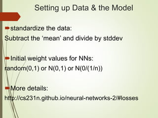
Setting up Data & the Model
ļ‚“standardize the data:
Subtract the ā€˜mean’ and divide by stddev
ļ‚“Initial weight values for NNs:
random(0,1) or N(0,1) or N(0/(1/n))
ļ‚“More details:
http://cs231n.github.io/neural-networks-2/#losses
Deep Neural Network: summary
ļ‚“ input layer, multiple hidden layers, and output layer
ļ‚“ nonlinear processing via activation functions
ļ‚“ perform transformation and feature extraction
ļ‚“ gradient descent algorithm with back propagation
ļ‚“ each layer receives the output from previous layer
ļ‚“ results are comparable/superior to human experts
Types of Deep Learning
ļ‚“ Supervised learning (you know the answer)
ļ‚“ unsupervised learning (you don’t know the answer)
ļ‚“ Semi-supervised learning (mixed dataset)
ļ‚“ Reinforcement learning (such as games)
ļ‚“ Types of algorithms:
ļ‚“ Classifiers (detect images, spam, fraud, etc)
ļ‚“ Regression (predict stock price, housing price, etc)
ļ‚“ Clustering (unsupervised classifiers)
CNNs versus RNNs
ļ‚“CNNs (Convolutional NNs):
Good for image processing
2000: CNNs processed 10-20% of all checks
=> Approximately 60% of all NNs
ļ‚“RNNs (Recurrent NNs):
Good for NLP and audio
Used in hybrid networks
CNNs: Convolution, ReLU, and Max Pooling
CNNs: Convolution Calculations
ļ‚“https://docs.gimp.org/en/plug-in-convmatrix.html
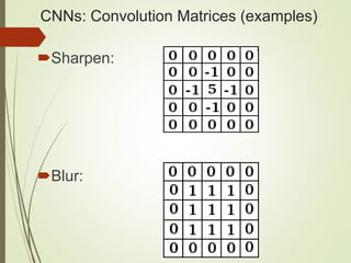
CNNs: Convolution Matrices (examples)
ļ‚“Sharpen:
ļ‚“Blur:
CNNs: Convolution Matrices (examples)
ļ‚“Edge detect:
ļ‚“Emboss:
CNNs: Max Pooling Example
GANs: Generative Adversarial Networks
ļ‚“Make imperceptible changes to images
ļ‚“Can consistently defeat all NNs
ļ‚“Can have extremely high error rate
ļ‚“Some images create optical illusions
ļ‚“https://www.quora.com/What-are-the-pros-and-cons-
of-using-generative-adversarial-networks-a-type-of-
neural-network
GANs: Generative Adversarial Networks
ļ‚“Create your own GANs:
https://www.oreilly.com/learning/generative-adversarial-networks-for-
beginners
https://github.com/jonbruner/generative-adversarial-networks
ļ‚“GANs from MNIST:
http://edwardlib.org/tutorials/gan
ļ‚“GANs and Capsule networks?
CNN in Python/Keras (fragment)
ļ‚“ from keras.models import Sequential
ļ‚“ from keras.layers.core import Dense, Dropout, Activation
ļ‚“ from keras.layers.convolutional import Conv2D, MaxPooling2D
ļ‚“ from keras.optimizers import Adadelta
ļ‚“ input_shape = (3, 32, 32)
ļ‚“ nb_classes = 10
ļ‚“ model = Sequential()
ļ‚“ model.add(Conv2D(32,(3, 3),padding='same’,
input_shape=input_shape))
ļ‚“ model.add(Activation('relu'))
ļ‚“ model.add(Conv2D(32, (3, 3)))
ļ‚“ model.add(Activation('relu'))
ļ‚“ model.add(MaxPooling2D(pool_size=(2, 2)))
ļ‚“ model.add(Dropout(0.25))
What is TensorFlow?
ļ‚“An open source framework for ML and DL
ļ‚“A ā€œcomputationā€ graph
ļ‚“Created by Google (released 11/2015)
ļ‚“Evolved from Google Brain
ļ‚“Linux and Mac OS X support (VM for Windows)
ļ‚“TF home page: https://www.tensorflow.org/
What is TensorFlow?
ļ‚“Support for Python, Java, C++
ļ‚“Desktop, server, mobile device (TensorFlow Lite)
ļ‚“CPU/GPU/TPU support
ļ‚“Visualization via TensorBoard
ļ‚“Can be embedded in Python scripts
ļ‚“Installation: pip install tensorflow
TensorFlow cluster:
https://www.tensorflow.org/deploy/distributed
TensorFlow Use Cases (Generic)
ļ‚“Image recognition
ļ‚“Computer vision
ļ‚“Voice/sound recognition
ļ‚“Time series analysis
ļ‚“Language detection
ļ‚“Language translation
ļ‚“Text-based processing
ļ‚“Handwriting Recognition
Aspects of TensorFlow
ļ‚“Graph: graph of operations (DAG)
ļ‚“Sessions: contains Graph(s)
ļ‚“lazy execution (default)
ļ‚“operations in parallel (default)
ļ‚“Nodes: operators/variables/constants
ļ‚“Edges: tensors
ļ‚“=> graphs are split into subgraphs and
executed in parallel (or multiple CPUs)
TensorFlow Graph Execution
ļ‚“Execute statements in a tf.Session() object
ļ‚“Invoke the ā€œrunā€ method of that object
ļ‚“ā€œeagerā€ execution is available (>= v1.4)
ļ‚“included in the mainline (v1.7)
ļ‚“Installation: pip install tensorflow
What is a Tensor?
ļ‚“TF tensors are n-dimensional arrays
ļ‚“TF tensors are very similar to numpy ndarrays
ļ‚“scalar number: a zeroth-order tensor
ļ‚“vector: a first-order tensor
ļ‚“matrix: a second-order tensor
ļ‚“3-dimensional array: a 3rd order tensor
ļ‚“https://dzone.com/articles/tensorflow-simplified-
examples
TensorFlow ā€œprimitive typesā€
ļ‚“tf.constant:
+ initialized immediately
+ immutable
ļ‚“tf.placeholder (a function):
+ initial value is not required
+ can have variable shape
+ assigned value via feed_dict at run time
+ receive data from ā€œexternalā€ sources
TensorFlow ā€œprimitive typesā€
ļ‚“tf.Variable (a class):
+ initial value is required
+ updated during training
+ maintain state across calls to ā€œrun()ā€
+ in-memory buffer (saved/restored from disk)
+ can be shared in a distributed environment
+ they hold learned parameters of a model
TensorFlow: constants (immutable)
ļ‚“ import tensorflow as tf
ļ‚“ aconst = tf.constant(3.0)
ļ‚“ print(aconst)
# output: Tensor("Const:0", shape=(), dtype=float32)
ļ‚“ sess = tf.Session()
ļ‚“ print(sess.run(aconst))
# output: 3.0
ļ‚“ sess.close()
ļ‚“ # => there's a better way
TensorFlow: constants
ļ‚“import tensorflow as tf
ļ‚“aconst = tf.constant(3.0)
ļ‚“print(aconst)
ļ‚“Automatically close ā€œsessā€
ļ‚“with tf.Session() as sess:
ļ‚“ print(sess.run(aconst))
TensorFlow Arithmetic
import tensorflow as tf
a = tf.add(4, 2)
b = tf.subtract(8, 6)
c = tf.multiply(a, 3)
d = tf.div(a, 6)
with tf.Session() as sess:
print(sess.run(a)) # 6
print(sess.run(b)) # 2
print(sess.run(c)) # 18
print(sess.run(d)) # 1
TensorFlow Arithmetic Methods
import tensorflow as tf
PI = 3.141592
sess = tf.Session()
print(sess.run(tf.div(12,8)))
print(sess.run(tf.floordiv(20.0,8.0)))
print(sess.run(tf.sin(PI)))
print(sess.run(tf.cos(PI)))
print(sess.run(tf.div(tf.sin(PI/4.),tf.cos(PI/4.))))
TensorFlow Arithmetic Methods
ļ‚“Output from previous slide:
ļ‚“1
ļ‚“2.0
ļ‚“6.27833e-07
ļ‚“-1.0
ļ‚“1.0
TF placeholders and feed_dict
import tensorflow as tf
a = tf.placeholder("float")
b = tf.placeholder("float")
c = tf.multiply(a,b)
# initialize a and b:
feed_dict = {a:2, b:3}
# multiply a and b:
with tf.Session() as sess:
print(sess.run(c, feed_dict))
TensorFlow: Simple Equation
ļ‚“import tensorflow as tf
ļ‚“# W and x are 1d arrays
ļ‚“W = tf.constant([10,20], name='W')
ļ‚“X = tf.placeholder(tf.int32, name='x')
ļ‚“b = tf.placeholder(tf.int32, name='b')
ļ‚“Wx = tf.multiply(W, x, name='Wx')
ļ‚“y = tf.add(Wx, b, name='y') OR
ļ‚“y2 = tf.add(tf.multiply(W,x),b)
TensorFlow fetch/feed_dict
with tf.Session() as sess:
print("Result 1: Wx = ",
sess.run(Wx, feed_dict={x:[5,10]}))
print("Result 2: y = ",
sess.run(y,feed_dict={x:[5,10],b:[15,25]}))
ļ‚“ Result 1: Wx = [50 200]
ļ‚“ Result 2: y = [65 225]
TensorFlow: Linear Regression
import tensorflow as tf
import numpy
rng = numpy.random
# tf Graph Input
X = tf.placeholder("float")
Y = tf.placeholder("float")
# Set model weights
W = tf.Variable(rng.randn(), name="weight")
b = tf.Variable(rng.randn(), name="bias")
# Construct a linear model (pred = predicted value):
pred = tf.add(tf.mul(X, W), b)
Saving Graphs for TensorBoard
import tensorflow as tf
x = tf.constant(5,name="x")
y = tf.constant(8,name="y")
z = tf.Variable(2*x+3*y, name="z")
init = tf.global_variables_initializer()
with tf.Session() as session:
writer = tf.summary.FileWriter("./tf_logs",session.graph)
session.run(init)
print 'z = ',session.run(z) # => z = 34
# launch: tensorboard –logdir=./tf_logs
TensorFlow Eager Execution
ļ‚“An imperative interface to TF
ļ‚“Fast debugging & immediate run-time errors
ļ‚“Eager execution is ā€œmainlineā€ in v1.7 of TF
ļ‚“=> requires Python 3.x (not Python 2.x)
TensorFlow Eager Execution
ļ‚“integration with Python tools
ļ‚“Supports dynamic models + Python control flow
ļ‚“support for custom and higher-order gradients
ļ‚“Supports most TensorFlow operations
ļ‚“https://research.googleblog.com/2017/10/eager-
execution-imperative-define-by.html
TensorFlow Eager Execution
ļ‚“import tensorflow as tf
ļ‚“import tensorflow.contrib.eager as tfe
ļ‚“tfe.enable_eager_execution()
ļ‚“x = [[2.]]
ļ‚“m = tf.matmul(x, x)
ļ‚“print(m)
# tf.Tensor([[4.]], shape=(1, 1), dtype=float32)
Deep Learning and Art/ā€Stuffā€
ļ‚“ā€œConvolutional Blendingā€ images:
=> 19-layer Convolutional Neural Network
www.deepart.io
ļ‚“https://www.fastcodesign.com/90124942/this-google-
engineer-taught-an-algorithm-to-make-train-footage-
and-its-hypnotic
Some of my Books
1) HTML5 Canvas and CSS3 Graphics (2013)
2) jQuery, CSS3, and HTML5 for Mobile (2013)
3) HTML5 Pocket Primer (2013)
4) jQuery Pocket Primer (2013)
5) HTML5 Mobile Pocket Primer (2014)
6) D3 Pocket Primer (2015)
7) Python Pocket Primer (2015)
8) SVG Pocket Primer (2016)
9) CSS3 Pocket Primer (2016)
10) Android Pocket Primer (2017)
11) Angular Pocket Primer (2017)
12) Data Cleaning Pocket Primer (2018)
13) RegEx Pocket Primer (2018)
What I do (Training)
=> Instructor at UCSC:
Deep Learning with TensorFlow (10/2018 & 02/2019)
Machine Learning Introduction (01/17/2019)
=> Mobile and TensorFlow Lite (WIP)
=> R and Deep Learning (WIP)
=> Android for Beginners (multi-day workshops)

Deep Learning and TensorFlow

  • 1.
    Introduction to DeepLearning BayPiggies Meetup 08/23/2018 LinkedIn Sunnyvale Unify Meeting Room Oswald Campesato ocampesato@yahoo.com
  • 2.
    Highlights/Overview ļ‚“intro to AI/ML/DL/NNs ļ‚“Hiddenlayers ļ‚“Initialization values ļ‚“Neurons per layer ļ‚“Activation function ļ‚“cost function ļ‚“gradient descent ļ‚“learning rate ļ‚“Dropout rate ļ‚“what are CNNs
  • 3.
  • 4.
    Use Cases forDeep Learning ļ‚“computer vision ļ‚“speech recognition ļ‚“image processing ļ‚“bioinformatics ļ‚“social network filtering ļ‚“drug design ļ‚“Recommendation systems ļ‚“Bioinformatics ļ‚“Mobile Advertising ļ‚“Many others
  • 5.
    NN 3 HiddenLayers: Classifier
  • 6.
    NN: 2 HiddenLayers (Regression)
  • 7.
  • 8.
    A Basic Modelin Machine Learning ļ‚“Let’s perform the following steps: ļ‚“1) Start with a simple model (2 variables) ļ‚“2) Generalize that model (n variables) ļ‚“3) See how it might apply to a NN
  • 9.
    Linear Regression ļ‚“One ofthe simplest models in ML ļ‚“Fits a line (y = m*x + b) to data in 2D ļ‚“Finds best line by minimizing MSE: m = slope of the best-fitting line b = y-intercept of the best-fitting line
  • 10.
  • 11.
  • 12.
  • 13.
    Linear Regression: example#1 ļ‚“One feature (independent variable): X = number of square feet ļ‚“Predicted value (dependent variable): Y = cost of a house ļ‚“A very ā€œcoarse grainedā€ model ļ‚“We can devise a much better model
  • 14.
    Linear Regression: example#2 ļ‚“Multiple features: ļ‚“X1 = # of square feet ļ‚“X2 = # of bedrooms ļ‚“X3 = # of bathrooms (dependency?) ļ‚“X4 = age of house ļ‚“X5 = cost of nearby houses ļ‚“X6 = corner lot (or not): Boolean ļ‚“a much better model (6 features)
  • 15.
    Linear Multivariate Analysis ļ‚“Generalform of multivariate equation: ļ‚“Y = w1*x1 + w2*x2 + . . . + wn*xn + b ļ‚“w1, w2, . . . , wn are numeric values ļ‚“x1, x2, . . . , xn are variables (features) ļ‚“Properties of variables: Can be independent (NaĆÆve Bayes) weak/strong dependencies can exist
  • 16.
    NN with 3Hidden Layers (again)
  • 17.
    Neural Networks: equations ļ‚“Nodeā€œvaluesā€ in first hidden layer: ļ‚“N1 = w11*x1+w21*x2+…+wn1*xn ļ‚“N2 = w12*x1+w22*x2+…+wn2*xn ļ‚“N3 = w13*x1+w23*x2+…+wn3*xn ļ‚“. . . ļ‚“Nn = w1n*x1+w2n*x2+…+wnn*xn ļ‚“Similar equations for other pairs of layers
  • 18.
    Neural Networks: Matrices ļ‚“Frominputs to first hidden layer: Y1 = W1*X + B1 (X/Y1/B1: vectors; W1: matrix) From first to second hidden layers: Y2 = W2*X + B2 (X/Y2/B2: vectors; W2: matrix) From second to third hidden layers: Y3 = W3*X + B3 (X/Y3/B3: vectors; W3: matrix)  Apply an ā€œactivation functionā€ to y values
  • 19.
    Neural Networks (general) ļ‚“Multiplehidden layers: Layer composition is your decision ļ‚“Activation functions: sigmoid, tanh, RELU https://en.wikipedia.org/wiki/Activation_function ļ‚“Back propagation (1980s) https://en.wikipedia.org/wiki/Backpropagation ļ‚“=> Initial weights: small random numbers
  • 20.
  • 21.
  • 22.
  • 23.
  • 24.
  • 25.
    Activation Functions inPython ļ‚“import numpy as np ļ‚“... ļ‚“# Python sigmoid example: ļ‚“z = 1/(1 + np.exp(-np.dot(W, x))) ļ‚“... ļ‚“# Python tanh example: ļ‚“z = np.tanh(np.dot(W,x)); ļ‚“# Python ReLU example: ļ‚“z = np.maximum(0, np.dot(W, x))
  • 26.
    What’s the ā€œBestā€Activation Function? ļ‚“Initially: sigmoid was popular ļ‚“Then: tanh became popular ļ‚“Now: RELU is preferred (better results) ļ‚“Softmax: for FC (fully connected) layers ļ‚“NB: sigmoid and tanh are used in LSTMs
  • 27.
    Types of Cost/ErrorFunctions ļ‚“MSE (mean-squared error) ļ‚“Cross-entropy ļ‚“exponential ļ‚“others
  • 28.
  • 29.
  • 30.
  • 31.
    How to Selecta Cost Function ļ‚“mean-squared error: for a regression problem ļ‚“binary cross-entropy (or mse): for a two-class classification problem ļ‚“categorical cross-entropy: for a many-class classification problem
  • 32.
  • 33.
    GD versus SGD ļ‚“SGD(Stochastic Gradient Descent): + one row of data ļ‚“Minibatch: involves a SUBSET of the dataset + aka Minibatch Stochastic Gradient Descent ļ‚“GD (Gradient Descent): + involves the ENTIRE dataset ļ‚“More details: http://cs229.stanford.edu/notes/cs229-notes1.pdf
  • 34.
    Setting up Data& the Model ļ‚“standardize the data: Subtract the ā€˜mean’ and divide by stddev ļ‚“Initial weight values for NNs: random(0,1) or N(0,1) or N(0/(1/n)) ļ‚“More details: http://cs231n.github.io/neural-networks-2/#losses
  • 35.
    Deep Neural Network:summary ļ‚“ input layer, multiple hidden layers, and output layer ļ‚“ nonlinear processing via activation functions ļ‚“ perform transformation and feature extraction ļ‚“ gradient descent algorithm with back propagation ļ‚“ each layer receives the output from previous layer ļ‚“ results are comparable/superior to human experts
  • 36.
    Types of DeepLearning ļ‚“ Supervised learning (you know the answer) ļ‚“ unsupervised learning (you don’t know the answer) ļ‚“ Semi-supervised learning (mixed dataset) ļ‚“ Reinforcement learning (such as games) ļ‚“ Types of algorithms: ļ‚“ Classifiers (detect images, spam, fraud, etc) ļ‚“ Regression (predict stock price, housing price, etc) ļ‚“ Clustering (unsupervised classifiers)
  • 37.
    CNNs versus RNNs ļ‚“CNNs(Convolutional NNs): Good for image processing 2000: CNNs processed 10-20% of all checks => Approximately 60% of all NNs ļ‚“RNNs (Recurrent NNs): Good for NLP and audio Used in hybrid networks
  • 38.
    CNNs: Convolution, ReLU,and Max Pooling
  • 39.
  • 40.
    CNNs: Convolution Matrices(examples) ļ‚“Sharpen: ļ‚“Blur:
  • 41.
    CNNs: Convolution Matrices(examples) ļ‚“Edge detect: ļ‚“Emboss:
  • 42.
  • 43.
  • 44.
    GANs: Generative AdversarialNetworks ļ‚“Make imperceptible changes to images ļ‚“Can consistently defeat all NNs ļ‚“Can have extremely high error rate ļ‚“Some images create optical illusions ļ‚“https://www.quora.com/What-are-the-pros-and-cons- of-using-generative-adversarial-networks-a-type-of- neural-network
  • 45.
    GANs: Generative AdversarialNetworks ļ‚“Create your own GANs: https://www.oreilly.com/learning/generative-adversarial-networks-for- beginners https://github.com/jonbruner/generative-adversarial-networks ļ‚“GANs from MNIST: http://edwardlib.org/tutorials/gan ļ‚“GANs and Capsule networks?
  • 46.
    CNN in Python/Keras(fragment) ļ‚“ from keras.models import Sequential ļ‚“ from keras.layers.core import Dense, Dropout, Activation ļ‚“ from keras.layers.convolutional import Conv2D, MaxPooling2D ļ‚“ from keras.optimizers import Adadelta ļ‚“ input_shape = (3, 32, 32) ļ‚“ nb_classes = 10 ļ‚“ model = Sequential() ļ‚“ model.add(Conv2D(32,(3, 3),padding='same’, input_shape=input_shape)) ļ‚“ model.add(Activation('relu')) ļ‚“ model.add(Conv2D(32, (3, 3))) ļ‚“ model.add(Activation('relu')) ļ‚“ model.add(MaxPooling2D(pool_size=(2, 2))) ļ‚“ model.add(Dropout(0.25))
  • 47.
    What is TensorFlow? ļ‚“Anopen source framework for ML and DL ļ‚“A ā€œcomputationā€ graph ļ‚“Created by Google (released 11/2015) ļ‚“Evolved from Google Brain ļ‚“Linux and Mac OS X support (VM for Windows) ļ‚“TF home page: https://www.tensorflow.org/
  • 48.
    What is TensorFlow? ļ‚“Supportfor Python, Java, C++ ļ‚“Desktop, server, mobile device (TensorFlow Lite) ļ‚“CPU/GPU/TPU support ļ‚“Visualization via TensorBoard ļ‚“Can be embedded in Python scripts ļ‚“Installation: pip install tensorflow TensorFlow cluster: https://www.tensorflow.org/deploy/distributed
  • 49.
    TensorFlow Use Cases(Generic) ļ‚“Image recognition ļ‚“Computer vision ļ‚“Voice/sound recognition ļ‚“Time series analysis ļ‚“Language detection ļ‚“Language translation ļ‚“Text-based processing ļ‚“Handwriting Recognition
  • 50.
    Aspects of TensorFlow ļ‚“Graph:graph of operations (DAG) ļ‚“Sessions: contains Graph(s) ļ‚“lazy execution (default) ļ‚“operations in parallel (default) ļ‚“Nodes: operators/variables/constants ļ‚“Edges: tensors ļ‚“=> graphs are split into subgraphs and executed in parallel (or multiple CPUs)
  • 51.
    TensorFlow Graph Execution ļ‚“Executestatements in a tf.Session() object ļ‚“Invoke the ā€œrunā€ method of that object ļ‚“ā€œeagerā€ execution is available (>= v1.4) ļ‚“included in the mainline (v1.7) ļ‚“Installation: pip install tensorflow
  • 52.
    What is aTensor? ļ‚“TF tensors are n-dimensional arrays ļ‚“TF tensors are very similar to numpy ndarrays ļ‚“scalar number: a zeroth-order tensor ļ‚“vector: a first-order tensor ļ‚“matrix: a second-order tensor ļ‚“3-dimensional array: a 3rd order tensor ļ‚“https://dzone.com/articles/tensorflow-simplified- examples
  • 53.
    TensorFlow ā€œprimitive typesā€ ļ‚“tf.constant: +initialized immediately + immutable ļ‚“tf.placeholder (a function): + initial value is not required + can have variable shape + assigned value via feed_dict at run time + receive data from ā€œexternalā€ sources
  • 54.
    TensorFlow ā€œprimitive typesā€ ļ‚“tf.Variable(a class): + initial value is required + updated during training + maintain state across calls to ā€œrun()ā€ + in-memory buffer (saved/restored from disk) + can be shared in a distributed environment + they hold learned parameters of a model
  • 55.
    TensorFlow: constants (immutable) ļ‚“import tensorflow as tf ļ‚“ aconst = tf.constant(3.0) ļ‚“ print(aconst) # output: Tensor("Const:0", shape=(), dtype=float32) ļ‚“ sess = tf.Session() ļ‚“ print(sess.run(aconst)) # output: 3.0 ļ‚“ sess.close() ļ‚“ # => there's a better way
  • 56.
    TensorFlow: constants ļ‚“import tensorflowas tf ļ‚“aconst = tf.constant(3.0) ļ‚“print(aconst) ļ‚“Automatically close ā€œsessā€ ļ‚“with tf.Session() as sess: ļ‚“ print(sess.run(aconst))
  • 57.
    TensorFlow Arithmetic import tensorflowas tf a = tf.add(4, 2) b = tf.subtract(8, 6) c = tf.multiply(a, 3) d = tf.div(a, 6) with tf.Session() as sess: print(sess.run(a)) # 6 print(sess.run(b)) # 2 print(sess.run(c)) # 18 print(sess.run(d)) # 1
  • 58.
    TensorFlow Arithmetic Methods importtensorflow as tf PI = 3.141592 sess = tf.Session() print(sess.run(tf.div(12,8))) print(sess.run(tf.floordiv(20.0,8.0))) print(sess.run(tf.sin(PI))) print(sess.run(tf.cos(PI))) print(sess.run(tf.div(tf.sin(PI/4.),tf.cos(PI/4.))))
  • 59.
    TensorFlow Arithmetic Methods ļ‚“Outputfrom previous slide: ļ‚“1 ļ‚“2.0 ļ‚“6.27833e-07 ļ‚“-1.0 ļ‚“1.0
  • 60.
    TF placeholders andfeed_dict import tensorflow as tf a = tf.placeholder("float") b = tf.placeholder("float") c = tf.multiply(a,b) # initialize a and b: feed_dict = {a:2, b:3} # multiply a and b: with tf.Session() as sess: print(sess.run(c, feed_dict))
  • 61.
    TensorFlow: Simple Equation ļ‚“importtensorflow as tf ļ‚“# W and x are 1d arrays ļ‚“W = tf.constant([10,20], name='W') ļ‚“X = tf.placeholder(tf.int32, name='x') ļ‚“b = tf.placeholder(tf.int32, name='b') ļ‚“Wx = tf.multiply(W, x, name='Wx') ļ‚“y = tf.add(Wx, b, name='y') OR ļ‚“y2 = tf.add(tf.multiply(W,x),b)
  • 62.
    TensorFlow fetch/feed_dict with tf.Session()as sess: print("Result 1: Wx = ", sess.run(Wx, feed_dict={x:[5,10]})) print("Result 2: y = ", sess.run(y,feed_dict={x:[5,10],b:[15,25]})) ļ‚“ Result 1: Wx = [50 200] ļ‚“ Result 2: y = [65 225]
  • 63.
    TensorFlow: Linear Regression importtensorflow as tf import numpy rng = numpy.random # tf Graph Input X = tf.placeholder("float") Y = tf.placeholder("float") # Set model weights W = tf.Variable(rng.randn(), name="weight") b = tf.Variable(rng.randn(), name="bias") # Construct a linear model (pred = predicted value): pred = tf.add(tf.mul(X, W), b)
  • 64.
    Saving Graphs forTensorBoard import tensorflow as tf x = tf.constant(5,name="x") y = tf.constant(8,name="y") z = tf.Variable(2*x+3*y, name="z") init = tf.global_variables_initializer() with tf.Session() as session: writer = tf.summary.FileWriter("./tf_logs",session.graph) session.run(init) print 'z = ',session.run(z) # => z = 34 # launch: tensorboard –logdir=./tf_logs
  • 65.
    TensorFlow Eager Execution ļ‚“Animperative interface to TF ļ‚“Fast debugging & immediate run-time errors ļ‚“Eager execution is ā€œmainlineā€ in v1.7 of TF ļ‚“=> requires Python 3.x (not Python 2.x)
  • 66.
    TensorFlow Eager Execution ļ‚“integrationwith Python tools ļ‚“Supports dynamic models + Python control flow ļ‚“support for custom and higher-order gradients ļ‚“Supports most TensorFlow operations ļ‚“https://research.googleblog.com/2017/10/eager- execution-imperative-define-by.html
  • 67.
    TensorFlow Eager Execution ļ‚“importtensorflow as tf ļ‚“import tensorflow.contrib.eager as tfe ļ‚“tfe.enable_eager_execution() ļ‚“x = [[2.]] ļ‚“m = tf.matmul(x, x) ļ‚“print(m) # tf.Tensor([[4.]], shape=(1, 1), dtype=float32)
  • 68.
    Deep Learning andArt/ā€Stuffā€ ļ‚“ā€œConvolutional Blendingā€ images: => 19-layer Convolutional Neural Network www.deepart.io ļ‚“https://www.fastcodesign.com/90124942/this-google- engineer-taught-an-algorithm-to-make-train-footage- and-its-hypnotic
  • 69.
    Some of myBooks 1) HTML5 Canvas and CSS3 Graphics (2013) 2) jQuery, CSS3, and HTML5 for Mobile (2013) 3) HTML5 Pocket Primer (2013) 4) jQuery Pocket Primer (2013) 5) HTML5 Mobile Pocket Primer (2014) 6) D3 Pocket Primer (2015) 7) Python Pocket Primer (2015) 8) SVG Pocket Primer (2016) 9) CSS3 Pocket Primer (2016) 10) Android Pocket Primer (2017) 11) Angular Pocket Primer (2017) 12) Data Cleaning Pocket Primer (2018) 13) RegEx Pocket Primer (2018)
  • 70.
    What I do(Training) => Instructor at UCSC: Deep Learning with TensorFlow (10/2018 & 02/2019) Machine Learning Introduction (01/17/2019) => Mobile and TensorFlow Lite (WIP) => R and Deep Learning (WIP) => Android for Beginners (multi-day workshops)