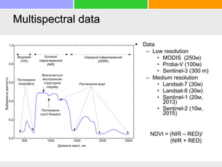
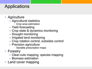
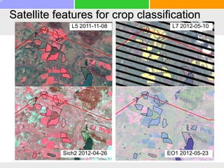
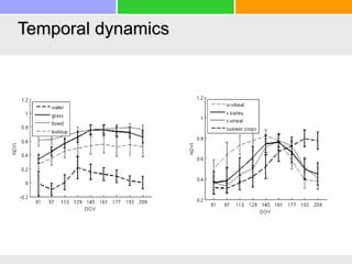
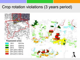
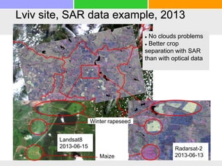
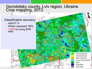
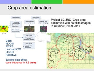
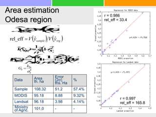
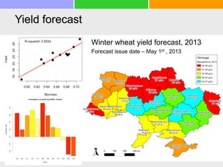
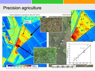
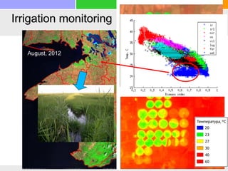
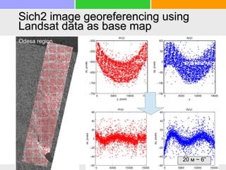
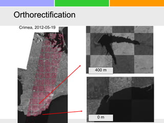
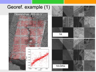
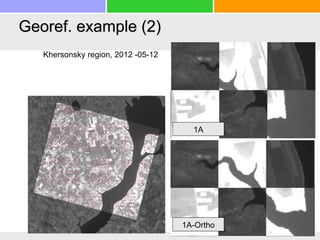
The document discusses the utilization of satellite imagery for agricultural monitoring and analysis, specifically in Ukraine. It details various satellite data resolutions and their applications in estimating crop areas, yield forecasting, and vegetation state assessment. The report includes information on data processing techniques, classification accuracy in crop mapping, and challenges related to geolocation errors and satellite image georeferencing.

1. Oleksiy Kravchenko
Senior Data Scientist, Zoral Labs, Kyiv

2. Satellite orbits

3. Geostationary satellite images - MSG

4. Polar orbiting images - MODIS

5. Multispectral data
 Data
– Low resolution
• MODIS (250м)
• Proba-V (100м)
• Sentinel-3 (300 m)
– Medium resolution
• Landsat-7 (30м)
• Landsat-8 (30м)
• Sentinel-1 (20м,
2013)
• Sentinel-2 (10м,
2015)
Довжина хвилі, нм
Відбиваючаздатність
Поглинання
хлорофілу Поглинання води
Поглинання
сухої біомаси
Визначається
внутрішньою
структурою
покриву
Видимий
(VIS)
Ближній
інфрачервоний
(NIR)
Середній інфрачервоний
(SWIR)
NDVI = (NIR – RED)/
(NIR + RED)

6. Applications
 Agriculture
– Agricultural statistics
• Crop area estimation
– Yield forecasting
– Crop state & dynamics monitoring
– Drought monitoring
– Irrigated land monitoring
– Crop rotation control, subsides control
– Precision agriculture
• Variable prescription maps
 Forestry
– Clear-cuts mapping, species mapping
– Biomass estimation
 Land cover mapping

7. 7
Satellite features for crop classification
L5 2011-11-08
EO1 2012-05-23
L7 2012-05-10
Sich2 2012-04-26

8. Temporal dynamics

9. Crop rotation violations (3 years period)
Rapeseed area
2011,2013: 490 ha
2011,2012: 430 ha
2012,2013: 435 ha
2013: 1540 ha
2012 2220 ha
2011 1610 ha

10. Lviv site, SAR data example, 2013
Landsat8
2013-06-15 Radarsat-2
2013-06-13
 No clouds problems
 Better crop
separation with SAR
than with optical data
Winter rapeseed
Maize

11. Gorodotsky county, Lviv region, Ukraine
Crop mapping, 2013
• Classification accuracy
– total 81 %
– Winter rapeseed: 96%
– +10% by using SAR
data

12. Crop area estimation
Project ЕС JRC “Crop area
estimation with satellite images
in Ukraine”, 2009-2011
Satellite data Ground data
Processing
· Orthorectification
· Segmentation
· Classification
Stratified Area
Frame Sampling
Along the road
survey
% pixels classified as cereals
%oatsingroundsurvey
SegmentsCrop field boundariesLC map
Area estimates
(pixel counting)
Data fusion
Adjustment of area
estimates
(Regression estimator)
Final results
· Area estimates
· Accuracy
assessment
Data:
MODIS
AWiFS
Landsat-5/TM
LISS-III
RapidEye
Satellite data effect:
costs decrease in 1.5 times

13. Area estimation
Odesa region
   regsample yVyV

rel_eff
  x yybxreg x 
 Vy
Nn
Nnn
G
n
reg
x
y()










 1
1
3
2
1
2
2
2 2

G
k
x
x
x
 3
3

 ( )Vy
nys rreg xy 
1
12 2
   regsample yVyV ˆˆrel_eff 
r = 0.986
rel_eff = 33.4
r = 0.997
rel_eff = 165.8
Data Area
th. ha
Error
(2σ)
ths. Ha
%
Sample 108.32 51.2 57.4%
MODIS 95.18 8.88 9.32%
Landsat 96.18 3.98 4.14%
Ministry
of Agric. 101,0 - -

14. Yield forecast
Winter wheat yield forecast, 2013
Forecast issue date – May 1st , 2013

15. Precision agriculture

16. Irrigation monitoring
August, 2012

17. Vegetation State Estimation (Forward &
Inverse Problems)
Leaf model
(PROSPECT)
Canopy RTM
(4SAIL)
Atmosphere RTM
(6S)
ll TR ,
3. Vegetation state
estimation using
radiometrically corrected
satellite data
Inverse problems
2. Vegetation state
estimation using satellite
data with atmospheric
correction
1. Vegetation state
estimation using in-situ
spectra
 ,, vs
soilR
lSLADLAI ,,
mwab CCCN, ,,
canopyR
TOAR
'
s
s
s
s
v
v s
dE
k E
dz
dE
a E E s E
dz
dE
a E E s E
dz
dE
K E E E w E
dz


 

 

 
 
 
     
      
        
1
( ) ( ) ( )i i ek K C k
N
   
90 1,90
,
90 1,901
N
N
N
R
R
R

 
 




 


18. Satellite product validation (crop state)
• Ukrainian GEO JECAM polygon
• Hemispherical photography (circular fisheye lenses)
LAI=0.22 fCover=16%
ALA=16º
LAI=4.0 fCover=79%
ALA=65º

19. Illegal cropping
znaydeno.com.ua
Illegal crops on 5.9 Ha, 7k hryvnas fines payed

20. Satellite image preprocessing.
Sentinel-2 example

21. Source: SPOT SATELLITE
GEOMETRY HANDBOOK, 2002
Direct model

22. Model parameters
• Time, location, velocity (satellite center mass), 1Hz
• Exterior attitude, 1Hz
– measured by star trackers
• Interior camera attitude within satellite coordinate system
– rotation matrix to align camera and star tracker
• Angular position of each pixel in camera coordinates
– Angular position of pixel assembly in focal plane
– Lenses distortion

23. Inverse model (RPC)

24. Direct model georeferensing of Sich2
satellite
• Geolocation error
– RapidEye (20-50 м)
– Landsat5 (30 м)
– Spot6,7 (10 м)
– Sich2 (200-700 м)
• Kyiv (240 м)
• Shatsk (550 м)
Shatsky National Park
Sich2, 2011-11-02
550m
USGS approach
for Landsat5

25. Drones georeferencing by telemetry
data only

26. Processing pipeline

27. Image based registration methods
Linear correlation surface Phase correlation
   
   
 
*
1 2
*
1 2
, ,
, ,
d dx y x y x x y y
x y x y
IM IM
e
IM IM
    
   



28. Phase correlation explained

40. Accuracy estimation

41. Linear vs. phase correlation
10-100 more control points

42. Odesa region
20 м ~ 6”
Sich2 image georeferencing using
Landsat data as base map

43. 400 m
0 m
Crimea, 2012-05-19
Orthorectification

44. 1A
1А-Orho
Zaporizhzhya, 2012-02-11
Georef. example (1)

45. Khersonsky region, 2012 -05-12
1A
1A-Ortho
Georef. example (2)

46. Pixel assembly calibration
Corrections.
Metadata
2011-10-03

47. Trend analysis Corrections
provided in metadata
2012-09-
05
After
launch
After
launch
1 year
on orbit
Pixel assembly coregistration (1)
1 year
on orbit

48. Band coregistration
PAN NIR
Along-track
shifts
DEM
SRTM

49. Jitter: Sich2 example
Roll oscillation
Amplitude ~ 4m
DI
Pitch oscillation
Amplitude ~ 2m
DI
DI, pixels

50. Jitter (2)
2011-10-05 2011-10-28

51. Reducing jitter
 SSTL, 2008
 Attitude Determination through
Registration of Earth Observational
Imagery
 Momentum Wheel Activation (Y-Axis) -
DU000373

52. Pixel assembly coregistration (1)
Sentinel-2
Pleiades

53. Pixel assembly coregistration (2)

54. Satellite image vs. aerial
registration
airplane
tracks
Distortions due to tall buildings

55. Questions?