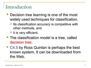
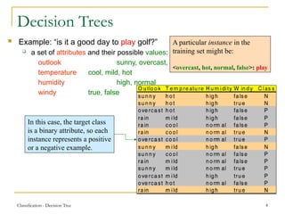
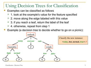
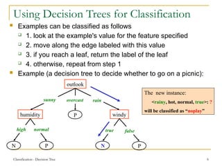
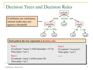
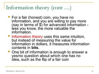
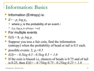
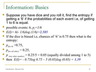
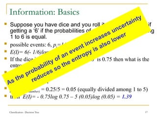
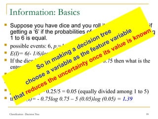
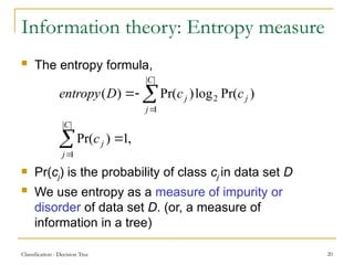
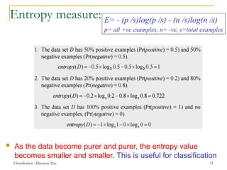
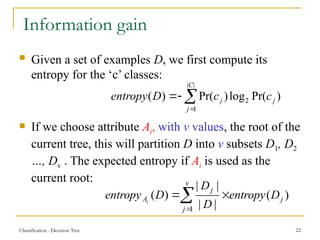
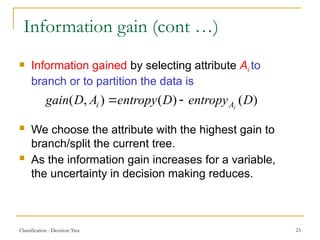
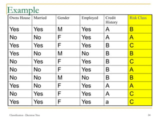
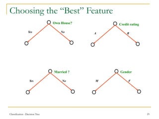
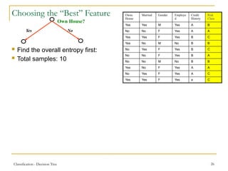
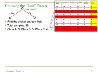
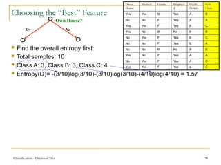
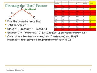
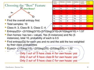
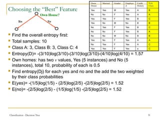
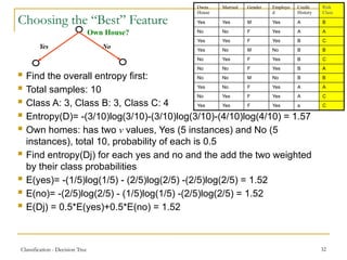
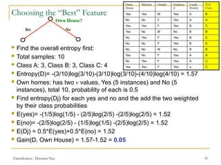
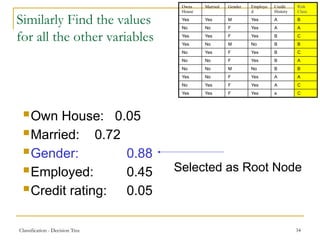
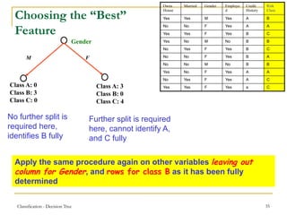
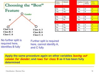
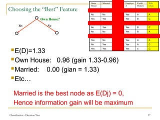
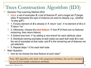
Supervised Learning:
Classification-I
Classification - Decision Tree 2
Decision tree induction
Classification - Decision Tree 3
Introduction
 Decision tree learning is one of the most
widely used techniques for classification.
 Its classification accuracy is competitive with
other methods, and
 it is very efficient.
 The classification model is a tree, called
decision tree.
 C4.5 by Ross Quinlan is perhaps the best
known system. It can be downloaded from
the Web.
Classification - Decision Tree 4
Decision Trees
 Example: “is it a good day to play golf?”
 a set of attributes and their possible values:
outlook sunny, overcast, rain
temperature cool, mild, hot
humidity high, normal
windy true, false
A particular instance in the
training set might be:
<overcast, hot, normal, false>: play
In this case, the target class
is a binary attribute, so each
instance represents a positive
or a negative example.
Classification - Decision Tree 5
Using Decision Trees for Classification
 Examples can be classified as follows
 1. look at the example's value for the feature specified
 2. move along the edge labeled with this value
 3. if you reach a leaf, return the label of the leaf
 4. otherwise, repeat from step 1
 Example (a decision tree to decide whether to go on a picnic):
outlook
humidity windy
P
P N P
N
sunny overcast rain
high normal true false
Classify the new instance:
<rainy, hot, normal, true>: ?
Classification - Decision Tree 6
Using Decision Trees for Classification
 Examples can be classified as follows
 1. look at the example's value for the feature specified
 2. move along the edge labeled with this value
 3. if you reach a leaf, return the label of the leaf
 4. otherwise, repeat from step 1
 Example (a decision tree to decide whether to go on a picnic):
outlook
humidity windy
P
P N P
N
sunny overcast rain
high normal true false
The new instance:
<rainy, hot, normal, true>: ?
will be classified as “noplay”
Classification - Decision Tree 7
Decision Trees and Decision Rules
outlook
humidity windy
yes
yes no yes
no
sunny overcast rain
> 75%<= 75% > 20 <= 20
If attributes are continuous,
internal nodes may test
against a threshold.
Rule1:
If (outlook=“sunny”) AND (humidity<=0.75)
Then (play=“yes”)
Rule2:
If (outlook=“rainy”) AND (wind>20)
Then (play=“no”)
Rule3:
If (outlook=“overcast”)
Then (play=“yes”)
. . .
Each path in the tree represents a decision rule:
Classification - Decision Tree 8
Top-Down Decision Tree Generation
 The basic approach usually consists of two phases:
 Tree construction
 At the start, all the training examples are at the
root
 Partition examples are recursively based on
selected attributes
 Tree pruning
 remove tree branches that may reflect noise in
the training data and lead to errors when
classifying test data
 improve classification accuracy
Classification - Decision Tree 9
Top-Down Decision Tree Generation
 Basic Steps in Decision Tree Construction
 Tree starts with a single node representing all data
 If samples are all from the same class then this
node becomes a leaf labeled with class label
 Otherwise, select feature that best separates
samples into individual classes.
 Recursion stops when:
 Samples in node belong to the same class
(majority)
 There are no remaining attributes on which to
split
How to select feature?
Classification - Decision Tree 10
How to find Feature to split?
 Many methods are available but our focus
will be on the following two:
 Information Theory
 Gini Index
Classification - Decision Tree 11
Information
No Uncertainty
High Uncertainty
Classification - Decision Tree 12
Valuable Information
 Which information is more valuable:
 Of high uncertain region, or
 Of no uncertain region
High Uncertain region
Classification - Decision Tree 13
Information theory
 Information theory provides a mathematical basis
for measuring the information content.
 To understand the notion of information, think
about it as providing the answer to a question, for
example, whether a coin will come up heads.
 If one already has a good guess about the answer,
then the actual answer is less informative.
 If one already knows that the coin is rigged so that it
will come with heads with probability 0.99, then a
message (advanced information) about the actual
outcome of a flip is worth less than it would be for a
honest coin (50-50).
Classification - Decision Tree 14
Information theory (cont …)
 For a fair (honest) coin, you have no
information, and you are willing to pay more
(say in terms of $) for advanced information -
less you know, the more valuable the
information.
 Information theory uses this same intuition,
but instead of measuring the value for
information in dollars, it measures information
contents in bits.
 One bit of information is enough to answer a
yes/no question about which one has no
idea, such as the flip of a fair coin
Classification - Decision Tree 15
Information: Basics
 Information (Entropy) is:
 E= - pi log pi,
 where pi is the probability of an event i
 (-pi log pi is always +ve)
 For multiple events
 E(I) = i -pi log pi
 Suppose you toss a fair coin, find the information
(entropy) when the probability of head or tail is 0.5 each.
 possible events: 2, pi=0.5
 E(I)= - 0.5log 0.5 - 0.5log 0.5 = 1.0
 If the coin is biased i.e, chances of heads is 0.75 and of tail
is 0.25, then E(I)= - 0.75log 0.75 - 0.25log 0.25 < 1.0
Classification - Decision Tree 16
Information: Basics
 Suppose you have dice and you roll it, find the entropy if
getting a ‘6’ if the probabilities of each event i.e, of getting
1 to 6 is equal.
 possible events: 6, pi=1/6
 E(I)= 6(- 1/6)log (1/6)=2.585
 If the dice is biased i.e, chances of ‘6’ is 0.75 then what is the
entropy:
 p(for 6) =0.75,
 p(for all other) = 0.25,
 p (any other number) = 0.25/5 = 0.05 (equally divided among 1 to 5)
 then E(I)= - 0.75log 0.75 – 5 (0.05)log (0.05) = 1.39
Classification - Decision Tree 17
Information: Basics
 Suppose you have dice and you roll it, find the entropy if
getting a ‘6’ if the probabilities of each event i.e, of getting
1 to 6 is equal.
 possible events: 6, pi=1/6
 E(I)= 6(- 1/6)log (1/6)=2.585
 If the dice is biased i.e, chances of ‘6’ is 0.75 then what is the
entropy:
 p(for 6) =0.75,
 p(for all other) = 0.25,
 p (any other number) = 0.25/5 = 0.05 (equally divided among 1 to 5)
 then E(I)= - 0.75log 0.75 – 5 (0.05)log (0.05) = 1.39
As the probability of an event increases uncertainty
reduces so the entropy is also lower
Classification - Decision Tree 18
Information: Basics
 Suppose you have dice and you roll it, find the entropy if
getting a ‘6’ if the probabilities of each event i.e, of getting
1 to 6 is equal.
 possible events: 6, pi=1/6
 E(I)= 6(- 1/6)log (1/6)=2.585
 If the dice is biased i.e, chances of ‘6’ is 0.75 then what is the
entropy:
 p(for 6) =0.75,
 p(for all other) = 0.25,
 p (any other number) = 0.25/5 = 0.05 (equally divided among 1 to 5)
 then E(I)= - 0.75log 0.75 – 5 (0.05)log (0.05) = 1.39
So in making a decision tree
choose a variable as the feature variable
that reduces the uncertainty once its value is known
Classification - Decision Tree 19
DT: Entropy – A measuring Value
 Entropy is a concept originated in thermodynamics
but later found its way to information theory.
 In decision tree construction process, definition of
entropy as a measure of disorder suits well.
 If the class values of the data in a node is equally
divided among possible values of the class value,
we say entropy (disorder) is maximum.
 If the class values of the data in a node is same for
all data, entropy (disorder) is minimum.
Classification - Decision Tree 20
Information theory: Entropy measure
 The entropy formula,
 Pr(cj) is the probability of class cj in data set D
 We use entropy as a measure of impurity or
disorder of data set D. (or, a measure of
information in a tree)
,
1
)
Pr(
)
Pr(
log
)
Pr(
)
(
|
|
1
|
|
1
2







C
j
j
j
C
j
j
c
c
c
D
entropy
Classification - Decision Tree 21
Entropy measure:
 As the data become purer and purer, the entropy value
becomes smaller and smaller. This is useful for classification
E= - (p /s)log(p /s) - (n /s)log(n /s)
p= all +ve examples, n= -ve, s=total examples
Classification - Decision Tree 22
Information gain
 Given a set of examples D, we first compute its
entropy for the ‘c’ classes:
 If we choose attribute Ai, with v values, the root of the
current tree, this will partition D into v subsets D1, D2
…, Dv . The expected entropy if Ai is used as the
current root:




v
j
j
j
A D
entropy
D
D
D
entropy i
1
)
(
|
|
|
|
)
(
)
Pr(
log
)
Pr(
)
(
|
|
1
2 j
C
j
j c
c
D
entropy 



Classification - Decision Tree 23
Information gain (cont …)
 Information gained by selecting attribute Ai to
branch or to partition the data is
 We choose the attribute with the highest gain to
branch/split the current tree.
 As the information gain increases for a variable,
the uncertainty in decision making reduces.
)
(
)
(
)
,
( D
entropy
D
entropy
A
D
gain i
A
i 

Classification - Decision Tree 24
Example
Owns House Married Gender Employed Credit
History
Risk Class
Yes Yes M Yes A B
No No F Yes A A
Yes Yes F Yes B C
Yes No M No B B
No Yes F Yes B C
No No F Yes B A
No No M No B B
Yes No F Yes A A
No Yes F Yes A C
Yes Yes F Yes a C
Classification - Decision Tree 25
Choosing the “Best” Feature
Gender
M F
Married ?
Yes No
Credit rating
A B
Own House?
Yes No
Classification - Decision Tree 26
Choosing the “Best” Feature
Own House?
Yes No
 Find the overall entropy first:
 Total samples: 10
Owns
House
Married Gender Employe
d
Credit
History
Risk
Class
Yes Yes M Yes A B
No No F Yes A A
Yes Yes F Yes B C
Yes No M No B B
No Yes F Yes B C
No No F Yes B A
No No M No B B
Yes No F Yes A A
No Yes F Yes A C
Yes Yes F Yes a C
Classification - Decision Tree 27
Choosing the “Best” Feature
Own House?
Yes No
 Find the overall entropy first:
 Total samples: 10
 Class A: 3, Class B: 3, Class C: 4
 Entropy(D)= -(3/10)log(3/10)-(3/10)log(3/10)-(4/10)log(4/10) = 1.57
 Own homes: has two v values, Yes (5 instances) and No (5
instances), total 10, probability of each is 0.5
 Find entropy(Dj) for each yes and no and the add the two weighted
by their class probabilities
 E(yes)= -(1/5)log(1/5) - (2/5)log(2/5) -(2/5)log(2/5) = 1.52
 E(no)= -(2/5)log(2/5) - (1/5)log(1/5) -(2/5)log(2/5) = 1.52
 E(Dj) = 0.5*E(yes)+0.5*E(no) = 1.52
 Gain(D, Own House) = 1.57-1.52 = 0.05
Owns
House
Married Gender Employe
d
Credit
History
Risk
Class
Yes Yes M Yes A B
No No F Yes A A
Yes Yes F Yes B C
Yes No M No B B
No Yes F Yes B C
No No F Yes B A
No No M No B B
Yes No F Yes A A
No Yes F Yes A C
Yes Yes F Yes a C
Classification - Decision Tree 28
Choosing the “Best” Feature
Own House?
Yes No
 Find the overall entropy first:
 Total samples: 10
 Class A: 3, Class B: 3, Class C: 4
 Entropy(D)= -(3/10)log(3/10)-(3/10)log(3/10)-(4/10)log(4/10) = 1.57
 Own homes: has two v values, Yes (5 instances) and No (5
instances), total 10, probability of each is 0.5
 Find entropy(Dj) for each yes and no and the add the two weighted
by their class probabilities
 E(yes)= -(1/5)log(1/5) - (2/5)log(2/5) -(2/5)log(2/5) = 1.52
 E(no)= -(2/5)log(2/5) - (1/5)log(1/5) -(2/5)log(2/5) = 1.52
 E(Dj) = 0.5*E(yes)+0.5*E(no) = 1.52
 Gain(D, Own House) = 1.57-1.52 = 0.05
Owns
House
Married Gender Employe
d
Credit
History
Risk
Class
Yes Yes M Yes A B
No No F Yes A A
Yes Yes F Yes B C
Yes No M No B B
No Yes F Yes B C
No No F Yes B A
No No M No B B
Yes No F Yes A A
No Yes F Yes A C
Yes Yes F Yes a C
Classification - Decision Tree 29
Choosing the “Best” Feature
Own House?
Yes No
 Find the overall entropy first:
 Total samples: 10
 Class A: 3, Class B: 3, Class C: 4
 Entropy(D)= -(3/10)log(3/10)-(3/10)log(3/10)-(4/10)log(4/10) = 1.57
 Own homes: has two v values, Yes (5 instances) and No (5
instances), total samples 10, probability of each is 0.5
 Find entropy(Dj) for each yes and no and the add the two weighted
by their class probabilities
 E(yes)= -(1/5)log(1/5) - (2/5)log(2/5) -(2/5)log(2/5) = 1.52
 E(no)= -(2/5)log(2/5) - (1/5)log(1/5) -(2/5)log(2/5) = 1.52
 E(Dj) = 0.5*E(yes)+0.5*E(no) = 1.52
 Gain(D, Own House) = 1.57-1.52 = 0.05
Owns
House
Married Gender Employe
d
Credit
History
Risk
Class
Yes Yes M Yes A B
No No F Yes A A
Yes Yes F Yes B C
Yes No M No B B
No Yes F Yes B C
No No F Yes B A
No No M No B B
Yes No F Yes A A
No Yes F Yes A C
Yes Yes F Yes a C
Classification - Decision Tree 30
Choosing the “Best” Feature
Own House?
Yes No
 Find the overall entropy first:
 Total samples: 10
 Class A: 3, Class B: 3, Class C: 4
 Entropy(D)= -(3/10)log(3/10)-(3/10)log(3/10)-(4/10)log(4/10) = 1.57
 Own homes: has two v values, Yes (5 instances) and No (5
instances), total 10, probability of each is 0.5
 Find entropy(Dj) for each yes and no and the add the two weighted
by their class probabilities
 E(yes)= -(1/5)log(1/5) - (2/5)log(2/5) -(2/5)log(2/5) = 1.52
 E(no)= -(2/5)log(2/5) - (1/5)log(1/5) -(2/5)log(2/5) = 1.52
 E(Dj) = 0.5*E(yes)+0.5*E(no) = 1.52
 Gain(D, Own House) = 1.57-1.52 = 0.05
Owns
House
Married Gender Employe
d
Credit
History
Risk
Class
Yes Yes M Yes A B
No No F Yes A A
Yes Yes F Yes B C
Yes No M No B B
No Yes F Yes B C
No No F Yes B A
No No M No B B
Yes No F Yes A A
No Yes F Yes A C
Yes Yes F Yes a C
Only 1 out of 5 have class A for own house: yes
Only 2 out of 5 have class B for own house: yes
Only 2 out of 5 have class C for own house: yes
Classification - Decision Tree 31
Choosing the “Best” Feature
Own House?
Yes No
 Find the overall entropy first:
 Total samples: 10
 Class A: 3, Class B: 3, Class C: 4
 Entropy(D)= -(3/10)log(3/10)-(3/10)log(3/10)-(4/10)log(4/10) = 1.57
 Own homes: has two v values, Yes (5 instances) and No (5
instances), total 10, probability of each is 0.5
 Find entropy(Dj) for each yes and no and the add the two weighted
by their class probabilities
 E(yes)= -(1/5)log(1/5) - (2/5)log(2/5) -(2/5)log(2/5) = 1.52
 E(no)= -(2/5)log(2/5) - (1/5)log(1/5) -(2/5)log(2/5) = 1.52
 E(Dj) = 0.5*E(yes)+0.5*E(no) = 1.52
 Gain(D, Own House) = 1.57-1.52 = 0.05
Owns
House
Married Gender Employe
d
Credit
History
Risk
Class
Yes Yes M Yes A B
No No F Yes A A
Yes Yes F Yes B C
Yes No M No B B
No Yes F Yes B C
No No F Yes B A
No No M No B B
Yes No F Yes A A
No Yes F Yes A C
Yes Yes F Yes a C
Classification - Decision Tree 32
Choosing the “Best” Feature
Own House?
Yes No
 Find the overall entropy first:
 Total samples: 10
 Class A: 3, Class B: 3, Class C: 4
 Entropy(D)= -(3/10)log(3/10)-(3/10)log(3/10)-(4/10)log(4/10) = 1.57
 Own homes: has two v values, Yes (5 instances) and No (5
instances), total 10, probability of each is 0.5
 Find entropy(Dj) for each yes and no and the add the two weighted
by their class probabilities
 E(yes)= -(1/5)log(1/5) - (2/5)log(2/5) -(2/5)log(2/5) = 1.52
 E(no)= -(2/5)log(2/5) - (1/5)log(1/5) -(2/5)log(2/5) = 1.52
 E(Dj) = 0.5*E(yes)+0.5*E(no) = 1.52
 Gain(D, Own House) = 1.57-1.52 = 0.05
Owns
House
Married Gender Employe
d
Credit
History
Risk
Class
Yes Yes M Yes A B
No No F Yes A A
Yes Yes F Yes B C
Yes No M No B B
No Yes F Yes B C
No No F Yes B A
No No M No B B
Yes No F Yes A A
No Yes F Yes A C
Yes Yes F Yes a C
Classification - Decision Tree 33
Choosing the “Best” Feature
Own House?
Yes No
 Find the overall entropy first:
 Total samples: 10
 Class A: 3, Class B: 3, Class C: 4
 Entropy(D)= -(3/10)log(3/10)-(3/10)log(3/10)-(4/10)log(4/10) = 1.57
 Own homes: has two v values, Yes (5 instances) and No (5
instances), total 10, probability of each is 0.5
 Find entropy(Dj) for each yes and no and the add the two weighted
by their class probabilities
 E(yes)= -(1/5)log(1/5) - (2/5)log(2/5) -(2/5)log(2/5) = 1.52
 E(no)= -(2/5)log(2/5) - (1/5)log(1/5) -(2/5)log(2/5) = 1.52
 E(Dj) = 0.5*E(yes)+0.5*E(no) = 1.52
 Gain(D, Own House) = 1.57-1.52 = 0.05
Owns
House
Married Gender Employe
d
Credit
History
Risk
Class
Yes Yes M Yes A B
No No F Yes A A
Yes Yes F Yes B C
Yes No M No B B
No Yes F Yes B C
No No F Yes B A
No No M No B B
Yes No F Yes A A
No Yes F Yes A C
Yes Yes F Yes a C
Classification - Decision Tree 34
Similarly Find the values
for all the other variables
Owns
House
Married Gender Employe
d
Credit
History
Risk
Class
Yes Yes M Yes A B
No No F Yes A A
Yes Yes F Yes B C
Yes No M No B B
No Yes F Yes B C
No No F Yes B A
No No M No B B
Yes No F Yes A A
No Yes F Yes A C
Yes Yes F Yes a C
Own House: 0.05
Married: 0.72
Gender: 0.88
Employed: 0.45
Credit rating: 0.05
Selected as Root Node
Classification - Decision Tree 35
Choosing the “Best”
Feature
Gender
M F
Class A: 3
Class B: 0
Class C: 4
Class A: 0
Class B: 3
Class C: 0
No further split is
required here,
identifies B fully
Further split is required
here, cannot identify A,
and C fully
Apply the same procedure again on other variables leaving out
column for Gender, and rows for class B as it has been fully
determined
Owns
House
Married Gender Employe
d
Credit
History
Risk
Class
Yes Yes M Yes A B
No No F Yes A A
Yes Yes F Yes B C
Yes No M No B B
No Yes F Yes B C
No No F Yes B A
No No M No B B
Yes No F Yes A A
No Yes F Yes A C
Yes Yes F Yes a C
Classification - Decision Tree 36
Choosing the “Best”
Feature
Gender
M F
Class A: 3
Class B: 0
Class C: 4
Class A: 0
Class B: 3
Class C: 0
No further split is
required here,
identifies B fully
Further split is required
here, cannot identify A,
and C fully
Apply the same procedure again on other variables leaving out
column for Gender, and rows for class B as it has been fully
determined
Owns
House
Married Gender Employe
d
Credit
History
Risk
Class
Yes Yes M Yes A B
No No F Yes A A
Yes Yes F Yes B C
Yes No M No B B
No Yes F Yes B C
No No F Yes B A
No No M No B B
Yes No F Yes A A
No Yes F Yes A C
Yes Yes F Yes a C
Classification - Decision Tree 37
Choosing the “Best” Feature
Own House?
Yes No
E(D)=1.33
Own House: 0.96 (gain 1.33-0.96)
Married: 0.00 (gian = 1.33)
Etc…
Owns
House
Married Gender Employe
d
Credit
History
Risk
Class
Yes Yes M Yes A B
No No F Yes A A
Yes Yes F Yes B C
Yes No M No B B
No Yes F Yes B C
No No F Yes B A
No No M No B B
Yes No F Yes A A
No Yes F Yes A C
Yes Yes F Yes a C
Married is the best node as E(Dj) = 0,
Hence information gain will be maximum
Classification - Decision Tree 38
Completing DT
Gender
M F
Class A: 3,Class C: 4
Class B: 3
Married
Yes No
Owns
House
Married Gender Employe
d
Credit
History
Risk
Class
Yes Yes M Yes A B
No No F Yes A A
Yes Yes F Yes B C
Yes No M No B B
No Yes F Yes B C
No No F Yes B A
No No M No B B
Yes No F Yes A A
No Yes F Yes A C
Yes Yes F Yes a C
Class C: 4 Class A: 3
Classification - Decision Tree 39
Completing DT
Owns
House
Married Gender Employe
d
Credit
History
Risk
Class
Yes Yes M Yes A B
No No F Yes A A
Yes Yes F Yes B C
Yes No M No B B
No Yes F Yes B C
No No F Yes B A
No No M No B B
Yes No F Yes A A
No Yes F Yes A C
Yes Yes F Yes a C
Gender
M F
Class A: 3,Class C: 4
Class B: 3
Married
Yes No
Class C: 4 Class A: 3
Rules
R1: If Gender=M then Class B
R2: If Gender=F and Married=Yes
Then Class C
R3: If Gender=F and Married=No
Then Class A
Classification - Decision Tree 40
Trees Construction Algorithm (ID3)
 Decision Tree Learning Method (ID3)
 Input: a set of examples S, a set of features F, and a target set T (target
class T represents the type of instance we want to classify, e.g., whether
“to play golf”)
 1. If every element of S is already in T, return “yes”; if no element of S is in
T return “no”
 2. Otherwise, choose the best feature f from F (if there are no features
remaining, then return failure);
 3. Extend tree from f by adding a new branch for each attribute value
 4. Distribute training examples to leaf nodes (so each leaf node S is now
the set of examples at that node, and F is the remaining set of features not
yet selected)
 5. Repeat steps 1-5 for each leaf node
 Main Question:
 how do we choose the best feature at each step?
Note: ID3 algorithm only deals with categorical attributes, but can be extended
(as in C4.5) to handle continuous attributes

Data Science-entropy machine learning.pptx

  • 1.
  • 2.
    Classification - DecisionTree 2 Decision tree induction
  • 3.
    Classification - DecisionTree 3 Introduction  Decision tree learning is one of the most widely used techniques for classification.  Its classification accuracy is competitive with other methods, and  it is very efficient.  The classification model is a tree, called decision tree.  C4.5 by Ross Quinlan is perhaps the best known system. It can be downloaded from the Web.
  • 4.
    Classification - DecisionTree 4 Decision Trees  Example: “is it a good day to play golf?”  a set of attributes and their possible values: outlook sunny, overcast, rain temperature cool, mild, hot humidity high, normal windy true, false A particular instance in the training set might be: <overcast, hot, normal, false>: play In this case, the target class is a binary attribute, so each instance represents a positive or a negative example.
  • 5.
    Classification - DecisionTree 5 Using Decision Trees for Classification  Examples can be classified as follows  1. look at the example's value for the feature specified  2. move along the edge labeled with this value  3. if you reach a leaf, return the label of the leaf  4. otherwise, repeat from step 1  Example (a decision tree to decide whether to go on a picnic): outlook humidity windy P P N P N sunny overcast rain high normal true false Classify the new instance: <rainy, hot, normal, true>: ?
  • 6.
    Classification - DecisionTree 6 Using Decision Trees for Classification  Examples can be classified as follows  1. look at the example's value for the feature specified  2. move along the edge labeled with this value  3. if you reach a leaf, return the label of the leaf  4. otherwise, repeat from step 1  Example (a decision tree to decide whether to go on a picnic): outlook humidity windy P P N P N sunny overcast rain high normal true false The new instance: <rainy, hot, normal, true>: ? will be classified as “noplay”
  • 7.
    Classification - DecisionTree 7 Decision Trees and Decision Rules outlook humidity windy yes yes no yes no sunny overcast rain > 75%<= 75% > 20 <= 20 If attributes are continuous, internal nodes may test against a threshold. Rule1: If (outlook=“sunny”) AND (humidity<=0.75) Then (play=“yes”) Rule2: If (outlook=“rainy”) AND (wind>20) Then (play=“no”) Rule3: If (outlook=“overcast”) Then (play=“yes”) . . . Each path in the tree represents a decision rule:
  • 8.
    Classification - DecisionTree 8 Top-Down Decision Tree Generation  The basic approach usually consists of two phases:  Tree construction  At the start, all the training examples are at the root  Partition examples are recursively based on selected attributes  Tree pruning  remove tree branches that may reflect noise in the training data and lead to errors when classifying test data  improve classification accuracy
  • 9.
    Classification - DecisionTree 9 Top-Down Decision Tree Generation  Basic Steps in Decision Tree Construction  Tree starts with a single node representing all data  If samples are all from the same class then this node becomes a leaf labeled with class label  Otherwise, select feature that best separates samples into individual classes.  Recursion stops when:  Samples in node belong to the same class (majority)  There are no remaining attributes on which to split How to select feature?
  • 10.
    Classification - DecisionTree 10 How to find Feature to split?  Many methods are available but our focus will be on the following two:  Information Theory  Gini Index
  • 11.
    Classification - DecisionTree 11 Information No Uncertainty High Uncertainty
  • 12.
    Classification - DecisionTree 12 Valuable Information  Which information is more valuable:  Of high uncertain region, or  Of no uncertain region High Uncertain region
  • 13.
    Classification - DecisionTree 13 Information theory  Information theory provides a mathematical basis for measuring the information content.  To understand the notion of information, think about it as providing the answer to a question, for example, whether a coin will come up heads.  If one already has a good guess about the answer, then the actual answer is less informative.  If one already knows that the coin is rigged so that it will come with heads with probability 0.99, then a message (advanced information) about the actual outcome of a flip is worth less than it would be for a honest coin (50-50).
  • 14.
    Classification - DecisionTree 14 Information theory (cont …)  For a fair (honest) coin, you have no information, and you are willing to pay more (say in terms of $) for advanced information - less you know, the more valuable the information.  Information theory uses this same intuition, but instead of measuring the value for information in dollars, it measures information contents in bits.  One bit of information is enough to answer a yes/no question about which one has no idea, such as the flip of a fair coin
  • 15.
    Classification - DecisionTree 15 Information: Basics  Information (Entropy) is:  E= - pi log pi,  where pi is the probability of an event i  (-pi log pi is always +ve)  For multiple events  E(I) = i -pi log pi  Suppose you toss a fair coin, find the information (entropy) when the probability of head or tail is 0.5 each.  possible events: 2, pi=0.5  E(I)= - 0.5log 0.5 - 0.5log 0.5 = 1.0  If the coin is biased i.e, chances of heads is 0.75 and of tail is 0.25, then E(I)= - 0.75log 0.75 - 0.25log 0.25 < 1.0
  • 16.
    Classification - DecisionTree 16 Information: Basics  Suppose you have dice and you roll it, find the entropy if getting a ‘6’ if the probabilities of each event i.e, of getting 1 to 6 is equal.  possible events: 6, pi=1/6  E(I)= 6(- 1/6)log (1/6)=2.585  If the dice is biased i.e, chances of ‘6’ is 0.75 then what is the entropy:  p(for 6) =0.75,  p(for all other) = 0.25,  p (any other number) = 0.25/5 = 0.05 (equally divided among 1 to 5)  then E(I)= - 0.75log 0.75 – 5 (0.05)log (0.05) = 1.39
  • 17.
    Classification - DecisionTree 17 Information: Basics  Suppose you have dice and you roll it, find the entropy if getting a ‘6’ if the probabilities of each event i.e, of getting 1 to 6 is equal.  possible events: 6, pi=1/6  E(I)= 6(- 1/6)log (1/6)=2.585  If the dice is biased i.e, chances of ‘6’ is 0.75 then what is the entropy:  p(for 6) =0.75,  p(for all other) = 0.25,  p (any other number) = 0.25/5 = 0.05 (equally divided among 1 to 5)  then E(I)= - 0.75log 0.75 – 5 (0.05)log (0.05) = 1.39 As the probability of an event increases uncertainty reduces so the entropy is also lower
  • 18.
    Classification - DecisionTree 18 Information: Basics  Suppose you have dice and you roll it, find the entropy if getting a ‘6’ if the probabilities of each event i.e, of getting 1 to 6 is equal.  possible events: 6, pi=1/6  E(I)= 6(- 1/6)log (1/6)=2.585  If the dice is biased i.e, chances of ‘6’ is 0.75 then what is the entropy:  p(for 6) =0.75,  p(for all other) = 0.25,  p (any other number) = 0.25/5 = 0.05 (equally divided among 1 to 5)  then E(I)= - 0.75log 0.75 – 5 (0.05)log (0.05) = 1.39 So in making a decision tree choose a variable as the feature variable that reduces the uncertainty once its value is known
  • 19.
    Classification - DecisionTree 19 DT: Entropy – A measuring Value  Entropy is a concept originated in thermodynamics but later found its way to information theory.  In decision tree construction process, definition of entropy as a measure of disorder suits well.  If the class values of the data in a node is equally divided among possible values of the class value, we say entropy (disorder) is maximum.  If the class values of the data in a node is same for all data, entropy (disorder) is minimum.
  • 20.
    Classification - DecisionTree 20 Information theory: Entropy measure  The entropy formula,  Pr(cj) is the probability of class cj in data set D  We use entropy as a measure of impurity or disorder of data set D. (or, a measure of information in a tree) , 1 ) Pr( ) Pr( log ) Pr( ) ( | | 1 | | 1 2        C j j j C j j c c c D entropy
  • 21.
    Classification - DecisionTree 21 Entropy measure:  As the data become purer and purer, the entropy value becomes smaller and smaller. This is useful for classification E= - (p /s)log(p /s) - (n /s)log(n /s) p= all +ve examples, n= -ve, s=total examples
  • 22.
    Classification - DecisionTree 22 Information gain  Given a set of examples D, we first compute its entropy for the ‘c’ classes:  If we choose attribute Ai, with v values, the root of the current tree, this will partition D into v subsets D1, D2 …, Dv . The expected entropy if Ai is used as the current root:     v j j j A D entropy D D D entropy i 1 ) ( | | | | ) ( ) Pr( log ) Pr( ) ( | | 1 2 j C j j c c D entropy    
  • 23.
    Classification - DecisionTree 23 Information gain (cont …)  Information gained by selecting attribute Ai to branch or to partition the data is  We choose the attribute with the highest gain to branch/split the current tree.  As the information gain increases for a variable, the uncertainty in decision making reduces. ) ( ) ( ) , ( D entropy D entropy A D gain i A i  
  • 24.
    Classification - DecisionTree 24 Example Owns House Married Gender Employed Credit History Risk Class Yes Yes M Yes A B No No F Yes A A Yes Yes F Yes B C Yes No M No B B No Yes F Yes B C No No F Yes B A No No M No B B Yes No F Yes A A No Yes F Yes A C Yes Yes F Yes a C
  • 25.
    Classification - DecisionTree 25 Choosing the “Best” Feature Gender M F Married ? Yes No Credit rating A B Own House? Yes No
  • 26.
    Classification - DecisionTree 26 Choosing the “Best” Feature Own House? Yes No  Find the overall entropy first:  Total samples: 10 Owns House Married Gender Employe d Credit History Risk Class Yes Yes M Yes A B No No F Yes A A Yes Yes F Yes B C Yes No M No B B No Yes F Yes B C No No F Yes B A No No M No B B Yes No F Yes A A No Yes F Yes A C Yes Yes F Yes a C
  • 27.
    Classification - DecisionTree 27 Choosing the “Best” Feature Own House? Yes No  Find the overall entropy first:  Total samples: 10  Class A: 3, Class B: 3, Class C: 4  Entropy(D)= -(3/10)log(3/10)-(3/10)log(3/10)-(4/10)log(4/10) = 1.57  Own homes: has two v values, Yes (5 instances) and No (5 instances), total 10, probability of each is 0.5  Find entropy(Dj) for each yes and no and the add the two weighted by their class probabilities  E(yes)= -(1/5)log(1/5) - (2/5)log(2/5) -(2/5)log(2/5) = 1.52  E(no)= -(2/5)log(2/5) - (1/5)log(1/5) -(2/5)log(2/5) = 1.52  E(Dj) = 0.5*E(yes)+0.5*E(no) = 1.52  Gain(D, Own House) = 1.57-1.52 = 0.05 Owns House Married Gender Employe d Credit History Risk Class Yes Yes M Yes A B No No F Yes A A Yes Yes F Yes B C Yes No M No B B No Yes F Yes B C No No F Yes B A No No M No B B Yes No F Yes A A No Yes F Yes A C Yes Yes F Yes a C
  • 28.
    Classification - DecisionTree 28 Choosing the “Best” Feature Own House? Yes No  Find the overall entropy first:  Total samples: 10  Class A: 3, Class B: 3, Class C: 4  Entropy(D)= -(3/10)log(3/10)-(3/10)log(3/10)-(4/10)log(4/10) = 1.57  Own homes: has two v values, Yes (5 instances) and No (5 instances), total 10, probability of each is 0.5  Find entropy(Dj) for each yes and no and the add the two weighted by their class probabilities  E(yes)= -(1/5)log(1/5) - (2/5)log(2/5) -(2/5)log(2/5) = 1.52  E(no)= -(2/5)log(2/5) - (1/5)log(1/5) -(2/5)log(2/5) = 1.52  E(Dj) = 0.5*E(yes)+0.5*E(no) = 1.52  Gain(D, Own House) = 1.57-1.52 = 0.05 Owns House Married Gender Employe d Credit History Risk Class Yes Yes M Yes A B No No F Yes A A Yes Yes F Yes B C Yes No M No B B No Yes F Yes B C No No F Yes B A No No M No B B Yes No F Yes A A No Yes F Yes A C Yes Yes F Yes a C
  • 29.
    Classification - DecisionTree 29 Choosing the “Best” Feature Own House? Yes No  Find the overall entropy first:  Total samples: 10  Class A: 3, Class B: 3, Class C: 4  Entropy(D)= -(3/10)log(3/10)-(3/10)log(3/10)-(4/10)log(4/10) = 1.57  Own homes: has two v values, Yes (5 instances) and No (5 instances), total samples 10, probability of each is 0.5  Find entropy(Dj) for each yes and no and the add the two weighted by their class probabilities  E(yes)= -(1/5)log(1/5) - (2/5)log(2/5) -(2/5)log(2/5) = 1.52  E(no)= -(2/5)log(2/5) - (1/5)log(1/5) -(2/5)log(2/5) = 1.52  E(Dj) = 0.5*E(yes)+0.5*E(no) = 1.52  Gain(D, Own House) = 1.57-1.52 = 0.05 Owns House Married Gender Employe d Credit History Risk Class Yes Yes M Yes A B No No F Yes A A Yes Yes F Yes B C Yes No M No B B No Yes F Yes B C No No F Yes B A No No M No B B Yes No F Yes A A No Yes F Yes A C Yes Yes F Yes a C
  • 30.
    Classification - DecisionTree 30 Choosing the “Best” Feature Own House? Yes No  Find the overall entropy first:  Total samples: 10  Class A: 3, Class B: 3, Class C: 4  Entropy(D)= -(3/10)log(3/10)-(3/10)log(3/10)-(4/10)log(4/10) = 1.57  Own homes: has two v values, Yes (5 instances) and No (5 instances), total 10, probability of each is 0.5  Find entropy(Dj) for each yes and no and the add the two weighted by their class probabilities  E(yes)= -(1/5)log(1/5) - (2/5)log(2/5) -(2/5)log(2/5) = 1.52  E(no)= -(2/5)log(2/5) - (1/5)log(1/5) -(2/5)log(2/5) = 1.52  E(Dj) = 0.5*E(yes)+0.5*E(no) = 1.52  Gain(D, Own House) = 1.57-1.52 = 0.05 Owns House Married Gender Employe d Credit History Risk Class Yes Yes M Yes A B No No F Yes A A Yes Yes F Yes B C Yes No M No B B No Yes F Yes B C No No F Yes B A No No M No B B Yes No F Yes A A No Yes F Yes A C Yes Yes F Yes a C Only 1 out of 5 have class A for own house: yes Only 2 out of 5 have class B for own house: yes Only 2 out of 5 have class C for own house: yes
  • 31.
    Classification - DecisionTree 31 Choosing the “Best” Feature Own House? Yes No  Find the overall entropy first:  Total samples: 10  Class A: 3, Class B: 3, Class C: 4  Entropy(D)= -(3/10)log(3/10)-(3/10)log(3/10)-(4/10)log(4/10) = 1.57  Own homes: has two v values, Yes (5 instances) and No (5 instances), total 10, probability of each is 0.5  Find entropy(Dj) for each yes and no and the add the two weighted by their class probabilities  E(yes)= -(1/5)log(1/5) - (2/5)log(2/5) -(2/5)log(2/5) = 1.52  E(no)= -(2/5)log(2/5) - (1/5)log(1/5) -(2/5)log(2/5) = 1.52  E(Dj) = 0.5*E(yes)+0.5*E(no) = 1.52  Gain(D, Own House) = 1.57-1.52 = 0.05 Owns House Married Gender Employe d Credit History Risk Class Yes Yes M Yes A B No No F Yes A A Yes Yes F Yes B C Yes No M No B B No Yes F Yes B C No No F Yes B A No No M No B B Yes No F Yes A A No Yes F Yes A C Yes Yes F Yes a C
  • 32.
    Classification - DecisionTree 32 Choosing the “Best” Feature Own House? Yes No  Find the overall entropy first:  Total samples: 10  Class A: 3, Class B: 3, Class C: 4  Entropy(D)= -(3/10)log(3/10)-(3/10)log(3/10)-(4/10)log(4/10) = 1.57  Own homes: has two v values, Yes (5 instances) and No (5 instances), total 10, probability of each is 0.5  Find entropy(Dj) for each yes and no and the add the two weighted by their class probabilities  E(yes)= -(1/5)log(1/5) - (2/5)log(2/5) -(2/5)log(2/5) = 1.52  E(no)= -(2/5)log(2/5) - (1/5)log(1/5) -(2/5)log(2/5) = 1.52  E(Dj) = 0.5*E(yes)+0.5*E(no) = 1.52  Gain(D, Own House) = 1.57-1.52 = 0.05 Owns House Married Gender Employe d Credit History Risk Class Yes Yes M Yes A B No No F Yes A A Yes Yes F Yes B C Yes No M No B B No Yes F Yes B C No No F Yes B A No No M No B B Yes No F Yes A A No Yes F Yes A C Yes Yes F Yes a C
  • 33.
    Classification - DecisionTree 33 Choosing the “Best” Feature Own House? Yes No  Find the overall entropy first:  Total samples: 10  Class A: 3, Class B: 3, Class C: 4  Entropy(D)= -(3/10)log(3/10)-(3/10)log(3/10)-(4/10)log(4/10) = 1.57  Own homes: has two v values, Yes (5 instances) and No (5 instances), total 10, probability of each is 0.5  Find entropy(Dj) for each yes and no and the add the two weighted by their class probabilities  E(yes)= -(1/5)log(1/5) - (2/5)log(2/5) -(2/5)log(2/5) = 1.52  E(no)= -(2/5)log(2/5) - (1/5)log(1/5) -(2/5)log(2/5) = 1.52  E(Dj) = 0.5*E(yes)+0.5*E(no) = 1.52  Gain(D, Own House) = 1.57-1.52 = 0.05 Owns House Married Gender Employe d Credit History Risk Class Yes Yes M Yes A B No No F Yes A A Yes Yes F Yes B C Yes No M No B B No Yes F Yes B C No No F Yes B A No No M No B B Yes No F Yes A A No Yes F Yes A C Yes Yes F Yes a C
  • 34.
    Classification - DecisionTree 34 Similarly Find the values for all the other variables Owns House Married Gender Employe d Credit History Risk Class Yes Yes M Yes A B No No F Yes A A Yes Yes F Yes B C Yes No M No B B No Yes F Yes B C No No F Yes B A No No M No B B Yes No F Yes A A No Yes F Yes A C Yes Yes F Yes a C Own House: 0.05 Married: 0.72 Gender: 0.88 Employed: 0.45 Credit rating: 0.05 Selected as Root Node
  • 35.
    Classification - DecisionTree 35 Choosing the “Best” Feature Gender M F Class A: 3 Class B: 0 Class C: 4 Class A: 0 Class B: 3 Class C: 0 No further split is required here, identifies B fully Further split is required here, cannot identify A, and C fully Apply the same procedure again on other variables leaving out column for Gender, and rows for class B as it has been fully determined Owns House Married Gender Employe d Credit History Risk Class Yes Yes M Yes A B No No F Yes A A Yes Yes F Yes B C Yes No M No B B No Yes F Yes B C No No F Yes B A No No M No B B Yes No F Yes A A No Yes F Yes A C Yes Yes F Yes a C
  • 36.
    Classification - DecisionTree 36 Choosing the “Best” Feature Gender M F Class A: 3 Class B: 0 Class C: 4 Class A: 0 Class B: 3 Class C: 0 No further split is required here, identifies B fully Further split is required here, cannot identify A, and C fully Apply the same procedure again on other variables leaving out column for Gender, and rows for class B as it has been fully determined Owns House Married Gender Employe d Credit History Risk Class Yes Yes M Yes A B No No F Yes A A Yes Yes F Yes B C Yes No M No B B No Yes F Yes B C No No F Yes B A No No M No B B Yes No F Yes A A No Yes F Yes A C Yes Yes F Yes a C
  • 37.
    Classification - DecisionTree 37 Choosing the “Best” Feature Own House? Yes No E(D)=1.33 Own House: 0.96 (gain 1.33-0.96) Married: 0.00 (gian = 1.33) Etc… Owns House Married Gender Employe d Credit History Risk Class Yes Yes M Yes A B No No F Yes A A Yes Yes F Yes B C Yes No M No B B No Yes F Yes B C No No F Yes B A No No M No B B Yes No F Yes A A No Yes F Yes A C Yes Yes F Yes a C Married is the best node as E(Dj) = 0, Hence information gain will be maximum
  • 38.
    Classification - DecisionTree 38 Completing DT Gender M F Class A: 3,Class C: 4 Class B: 3 Married Yes No Owns House Married Gender Employe d Credit History Risk Class Yes Yes M Yes A B No No F Yes A A Yes Yes F Yes B C Yes No M No B B No Yes F Yes B C No No F Yes B A No No M No B B Yes No F Yes A A No Yes F Yes A C Yes Yes F Yes a C Class C: 4 Class A: 3
  • 39.
    Classification - DecisionTree 39 Completing DT Owns House Married Gender Employe d Credit History Risk Class Yes Yes M Yes A B No No F Yes A A Yes Yes F Yes B C Yes No M No B B No Yes F Yes B C No No F Yes B A No No M No B B Yes No F Yes A A No Yes F Yes A C Yes Yes F Yes a C Gender M F Class A: 3,Class C: 4 Class B: 3 Married Yes No Class C: 4 Class A: 3 Rules R1: If Gender=M then Class B R2: If Gender=F and Married=Yes Then Class C R3: If Gender=F and Married=No Then Class A
  • 40.
    Classification - DecisionTree 40 Trees Construction Algorithm (ID3)  Decision Tree Learning Method (ID3)  Input: a set of examples S, a set of features F, and a target set T (target class T represents the type of instance we want to classify, e.g., whether “to play golf”)  1. If every element of S is already in T, return “yes”; if no element of S is in T return “no”  2. Otherwise, choose the best feature f from F (if there are no features remaining, then return failure);  3. Extend tree from f by adding a new branch for each attribute value  4. Distribute training examples to leaf nodes (so each leaf node S is now the set of examples at that node, and F is the remaining set of features not yet selected)  5. Repeat steps 1-5 for each leaf node  Main Question:  how do we choose the best feature at each step? Note: ID3 algorithm only deals with categorical attributes, but can be extended (as in C4.5) to handle continuous attributes