This document help you to learn about machine learning

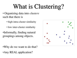
1. • Organizing data into clusters
such that there is
• high intra-cluster similarity
• low inter-cluster similarity
•Informally, finding natural
groupings among objects.
•Why do we want to do that?
•Any REAL application?
What is Clustering?

2. Example: clusty

3. Example: clustering genes
• Microarrays measures the activities
of all genes in different conditions
• Clustering genes can help determine
new functions for unknown genes
• An early “killer application” in this
area
– The most cited (11,591) paper in
PNAS!

4. Why clustering?
• Organizing data into clusters provides information
about the internal structure of the data
– Ex. Clusty and clustering genes above
• Sometimes the partitioning is the goal
– Ex. Image segmentation
• Knowledge discovery in data
– Ex. Underlying rules, reoccurring patterns, topics, etc.

5. Unsupervised learning
• Clustering methods are unsupervised learning
techniques
- We do not have a teacher that provides examples with their
labels
• We will also discuss dimensionality reduction,
another unsupervised learning method later in the
course

6. Outline
•Motivation
•Distance functions
•Hierarchical clustering
•Partitional clustering
– K-means
– Gaussian Mixture Models
•Number of clusters

7. What is a natural grouping among these objects?

8. School Employees
Simpson's Family Males
Females
Clustering is subjective
What is a natural grouping among these objects?

9. What is Similarity?
The quality or state of being similar; likeness; resemblance; as, a similarity of features.
Similarity is hard
to define, but…
“We know it when
we see it”
The real meaning
of similarity is a
philosophical
question. We will
take a more
pragmatic
approach.
Webster's Dictionary

10. Defining Distance Measures
Definition: Let O1 and O2 be two objects from the
universe of possible objects. The distance (dissimilarity)
between O1 and O2 is a real number denoted by D(O1,O2)
0.23 3 342.7
gene2
gene1

11. A few examples:
• Euclidian distance
• Correlation coefficient
3
d('', '') = 0 d(s, '') =
d('', s) = |s| -- i.e.
length of s d(s1+ch1,
s2+ch2) = min( d(s1,
s2) + if ch1=ch2 then
0 else 1 fi, d(s1+ch1,
s2) + 1, d(s1,
s2+ch2) + 1 )
Inside these black boxes:
some function on two variables
(might be simple or very
complex)
gene2
gene1
d(x,y)  (xi  yi)2
i

s(x,y) 
(xi x )(yi y )
i

xy
• Similarity rather than distance
• Can determine similar trends

12. Outline
•Motivation
•Distance measure
•Hierarchical clustering
•Partitional clustering
– K-means
– Gaussian Mixture Models
•Number of clusters

13. Desirable Properties of a Clustering Algorithm
• Scalability (in terms of both time and space)
• Ability to deal with different data types
• Minimal requirements for domain knowledge to
determine input parameters
• Interpretability and usability
Optional
- Incorporation of user-specified constraints

14. Two Types of Clustering
Hierarchical
• Partitional algorithms: Construct various partitions and then
evaluate them by some criterion
• Hierarchical algorithms: Create a hierarchical decomposition of
the set of objects using some criterion (focus of this class)
Partitional
Top down
Bottom up or top down

15. (How-to) Hierarchical Clustering
The number of dendrograms with n
leafs = (2n -3)!/[(2(n -2)) (n -2)!]
Number Number of Possible
of Leafs Dendrograms
2 1
3 3
4 15
5 105
... …
10 34,459,425
Bottom-Up (agglomerative): Starting
with each item in its own cluster, find
the best pair to merge into a new cluster.
Repeat until all clusters are fused
together.

16. 0 8 8 7 7
0 2 4 4
0 3 3
0 1
0
D( , ) = 8
D( , ) = 1
We begin with a distance
matrix which contains the
distances between every pair
of objects in our database.

17. Bottom-Up (agglomerative):
Starting with each item in its own
cluster, find the best pair to merge into
a new cluster. Repeat until all clusters
are fused together.
…
Consider all
possible
merges…
Choose
the best

18. Bottom-Up (agglomerative):
Starting with each item in its own
cluster, find the best pair to merge into
a new cluster. Repeat until all clusters
are fused together.
…
Consider all
possible
merges…
Choose
the best
Consider all
possible
merges… …
Choose
the best

19. Bottom-Up (agglomerative):
Starting with each item in its own
cluster, find the best pair to merge into
a new cluster. Repeat until all clusters
are fused together.
…
Consider all
possible
merges…
Choose
the best
Consider all
possible
merges… …
Choose
the best
Consider all
possible
merges…
Choose
the best
…

20. Bottom-Up (agglomerative):
Starting with each item in its own
cluster, find the best pair to merge into
a new cluster. Repeat until all clusters
are fused together.
…
Consider all
possible
merges…
Choose
the best
Consider all
possible
merges… …
Choose
the best
Consider all
possible
merges…
Choose
the best
…
But how do we compute distances
between clusters rather than
objects?

21. Computing distance between
clusters: Single Link
• cluster distance = distance of two closest
members in each class
- Potentially
long and skinny
clusters

22. Example: single link
















0
4
5
8
9
0
7
9
10
0
3
6
0
2
0
5
4
3
2
1
5
4
3
2
1
1
2
3
4
5

23. Example: single link
















0
4
5
8
9
0
7
9
10
0
3
6
0
2
0
5
4
3
2
1
5
4
3
2
1












0
4
5
8
0
7
9
0
3
0
5
4
3
)
2
,
1
(
5
4
3
)
2
,
1
(
1
2
3
4
5
8
}
8
,
9
min{
}
,
min{
9
}
9
,
10
min{
}
,
min{
3
}
3
,
6
min{
}
,
min{
5
,
2
5
,
1
5
),
2
,
1
(
4
,
2
4
,
1
4
),
2
,
1
(
3
,
2
3
,
1
3
),
2
,
1
(









d
d
d
d
d
d
d
d
d

24. Example: single link










0
4
5
0
7
0
5
4
)
3
,
2
,
1
(
5
4
)
3
,
2
,
1
(
1
2
3
4
5












0
4
5
8
0
7
9
0
3
0
5
4
3
)
2
,
1
(
5
4
3
)
2
,
1
(
















0
4
5
8
9
0
7
9
10
0
3
6
0
2
0
5
4
3
2
1
5
4
3
2
1
5
}
5
,
8
min{
}
,
min{
7
}
7
,
9
min{
}
,
min{
5
,
3
5
),
2
,
1
(
5
),
3
,
2
,
1
(
4
,
3
4
),
2
,
1
(
4
),
3
,
2
,
1
(






d
d
d
d
d
d

25. Example: single link










0
4
5
0
7
0
5
4
)
3
,
2
,
1
(
5
4
)
3
,
2
,
1
(
1
2
3
4
5












0
4
5
8
0
7
9
0
3
0
5
4
3
)
2
,
1
(
5
4
3
)
2
,
1
(
















0
4
5
8
9
0
7
9
10
0
3
6
0
2
0
5
4
3
2
1
5
4
3
2
1
5
}
,
min{ 5
),
3
,
2
,
1
(
4
),
3
,
2
,
1
(
)
5
,
4
(
),
3
,
2
,
1
( 
 d
d
d

26. Computing distance between
clusters: : Complete Link
• cluster distance = distance of two farthest
members
+ tight clusters

27. Computing distance between
clusters: Average Link
• cluster distance = average distance of all
pairs
the most widely
used measure
Robust against
noise

28. 29 2 6 11 9 17 10 13 24 25 26 20 22 30 27 1 3 8 4 12 5 14 23 15 16 18 19 21 28 7
1
2
3
4
5
6
7
Average linkage
Single linkage
Height represents
distance between objects
/ clusters

31. Summary of Hierarchal Clustering Methods
• No need to specify the number of clusters in
advance.
• Hierarchical structure maps nicely onto human
intuition for some domains
• They do not scale well: time complexity of at least
O(n2), where n is the number of total objects.
• Like any heuristic search algorithms, local optima
are a problem.
• Interpretation of results is (very) subjective.

32. In some cases we can determine the “correct” number of clusters.
However, things are rarely this clear cut, unfortunately.
But what are the clusters?

33. Outlier
One potential use of a dendrogram is to detect outliers
The single isolated branch is suggestive of a
data point that is very different to all others

34. Example: clustering genes
• Microarrays measures the activities of all
genes in different conditions
• Clustering genes can help determine new
functions for unknown genes

35. Partitional Clustering
• Nonhierarchical, each instance is placed in
exactly one of K non-overlapping clusters.
• Since the output is only one set of clusters the
user has to specify the desired number of
clusters K.

36. 0
1
2
3
4
5
0 1 2 3 4 5
K-means Clustering: Initialization
Decide K, and initialize K centers (randomly)
k1
k2
k3

37. 0
1
2
3
4
5
0 1 2 3 4 5
K-means Clustering: Iteration 1
Assign all objects to the nearest center.
Move a center to the mean of its members.
k1
k2
k3

38. 0
1
2
3
4
5
0 1 2 3 4 5
K-means Clustering: Iteration 2
After moving centers, re-assign the objects…
k1
k2
k3

39. 0
1
2
3
4
5
0 1 2 3 4 5
K-means Clustering: Iteration 2
k1
k2
k3
After moving centers, re-assign the objects to nearest centers.
Move a center to the mean of its new members.

40. 0
1
2
3
4
5
0 1 2 3 4 5
K-means Clustering: Finished!
Re-assign and move centers, until …
no objects changed membership.
k1
k2
k3

41. Algorithm k-means
1. Decide on a value for K, the number of clusters.
2. Initialize the K cluster centers (randomly, if
necessary).
3. Decide the class memberships of the N objects by
assigning them to the nearest cluster center.
4. Re-estimate the K cluster centers, by assuming the
memberships found above are correct.
5. Repeat 3 and 4 until none of the N objects changed
membership in the last iteration.

42. Algorithm k-means
1. Decide on a value for K, the number of clusters.
2. Initialize the K cluster centers (randomly, if
necessary).
3. Decide the class memberships of the N objects by
assigning them to the nearest cluster center.
4. Re-estimate the K cluster centers, by assuming the
memberships found above are correct.
5. Repeat 3 and 4 until none of the N objects changed
membership in the last iteration.
Use one of the distance /
similarity functions we
discussed earlier
Average / median of class
members

43. Summary: K-Means
• Strength
– Simple, easy to implement and debug
– Intuitive objective function: optimizes intra-cluster similarity
– Relatively efficient: O(tkn), where n is # objects, k is # clusters,
and t is # iterations. Normally, k, t << n.
• Weakness
– Applicable only when mean is defined, what about categorical
data?
– Often terminates at a local optimum. Initialization is important.
– Need to specify K, the number of clusters, in advance
– Unable to handle noisy data and outliers
– Not suitable to discover clusters with non-convex shapes
• Summary
– Assign members based on current centers
– Re-estimate centers based on current assignment

44. 10
1 2 3 4 5 6 7 8 9 10
1
2
3
4
5
6
7
8
9
How can we tell the right number of clusters?
In general, this is a unsolved problem. However there are many
approximate methods. In the next few slides we will see an example.

45. 1 2 3 4 5 6 7 8 9 10
When k = 1, the objective function is 873.0

46. 1 2 3 4 5 6 7 8 9 10
When k = 2, the objective function is 173.1

47. 1 2 3 4 5 6 7 8 9 10
When k = 3, the objective function is 133.6

48. 0.00E+00
1.00E+02
2.00E+02
3.00E+02
4.00E+02
5.00E+02
6.00E+02
7.00E+02
8.00E+02
9.00E+02
1.00E+03
1 2 3 4 5 6
We can plot the objective function values for k equals 1 to 6…
The abrupt change at k = 2, is highly suggestive of two clusters
in the data. This technique for determining the number of
clusters is known as “knee finding” or “elbow finding”.
Note that the results are not always as clear cut as in this toy example
k
Objective
Function

49. DBSCAN
(Density-Based Spatial Clustering and Application with Noise)
Source: www.sthda.com
DBSCAN is a density-based clusering algorithm, introduced in Ester et al. 1996,
which can be used to identify clusters of any shape in a data set containing
noise and outliers.
The basic idea behind the density-based clustering approach is derived from a
human intuitive clustering method. For instance, by looking at the figure below,
one can easily identify four clusters along with several points of noise, because
of the differences in the density of points.
The key idea is that for each point of a cluster, the neighborhood of a given
radius has to contain at least a minimum number of points.

50. Why DBSCAN
Partitioning methods (K-means, PAM clustering) and hierarchical clustering are
suitable for finding spherical-shaped clusters or convex clusters. In other words,
they work well only for compact and well separated clusters. Moreover, they are
also severely affected by the presence of noise and outliers in the data.
Unfortunately, real life data can contain: i) clusters of arbitrary shape such as
those shown in the figure below (oval, linear and “S” shape clusters); ii) many
outliers and noise.
The figure below shows a data set containing nonconvex clusters and
outliers/noises.

51. DBSCAN Algorithm
The goal is to identify dense regions, which can be measured by the number of
objects close to a given point.
Two important parameters are required for DBSCAN: epsilon (“eps”) and
minimum points (“MinPts”). The parameter eps defines the radius of
neighborhood around a point x. It’s called called the eps-neighborhood of x. The
parameter MinPts is the minimum number of neighbors within “eps” radius.
Any point x in the data set, with a neighbor count greater than or equal to
MinPts, is marked as a core point. We say that x is border point, if the
number of its neighbors is less than MinPts, but it belongs to the eps-
neighborhood of some core point z. Finally, if a point is neither a core nor a
border point, then it is called a noise point or an outlier.

52. DBSCAN Algorithm
We start by defining 3 terms:
Direct density reachable: A point “A” is directly density reachable from
another point “B” if: i) “A” is in the eps-neighborhood of “B” and ii) “B” is a core
point. Example: ‘p’ and ‘m’; ‘q’ and ‘m’
Density reachable: A point “A” is density reachable from “B” if there are a set
of core points leading from “B” to “A. Example: ‘s’ and ‘r’.
Density connected: Two points “A” and “B” are density connected if there are
a core point “C”, such that both “A” and “B” are density reachable from “C”.
Example: ‘p’ and ‘q’;

53. DBSCAN Algorithm

54. DBSCAN Algorithm

55. BIRCH (Balanced Iterative Reducing and
Clustering using Hierarchies)
??