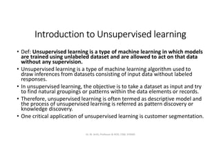
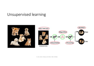
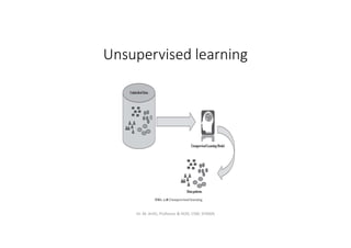
Interactive Powerpoint_How to Master effective communication
Unit 5-1.pdf
1. Unit 5
Clustering
Dr. M. Arthi
Professor & HOD
Department of CSE-AIML
Sreenivasa Institute of Technology and Management Studies
2. Introduction to Unsupervised learning
• Def: Unsupervised learning is a type of machine learning in which models
are trained using unlabeled dataset and are allowed to act on that data
without any supervision.
• Unsupervised learning is a type of machine learning algorithm used to
draw inferences from datasets consisting of input data without labeled
responses.
• In unsupervised learning, the objective is to take a dataset as input and try
to find natural groupings or patterns within the data elements or records.
• Therefore, unsupervised learning is often termed as descriptive model and
the process of unsupervised learning is referred as pattern discovery or
knowledge discovery.
• One critical application of unsupervised learning is customer segmentation.
Dr. M. Arthi, Professor & HOD, CSM, SITAMS
4. Why use Unsupervised Learning
• Unsupervised learning is helpful for finding useful insights from the
data.
• Unsupervised learning is much similar as a human learns to think by
their own experiences, which makes it closer to the real AI.
• Unsupervised learning works on unlabeled and uncategorized data
which make unsupervised learning more important.
• In real-world, we do not always have input data with the
corresponding output so to solve such cases, we need unsupervised
learning.
Dr. M. Arthi, Professor & HOD, CSM, SITAMS
6. Unsupervised learning- Clustering
• Different measures of similarity can be applied for clustering.
• One of the most commonly adopted similarity measure is distance.
• Two data items are considered as a part of the same cluster if the
distance between them is less.
• In the same way, if the distance between the data items is high, the
items do not generally belong to the same cluster.
• This is also known as distance-based clustering.
Dr. M. Arthi, Professor & HOD, CSM, SITAMS
8. Unsupervised learning- Association analysis
• Other than clustering of data and getting a summarized view from it, one
more variant of unsupervised learning is association analysis.
• As a part of association analysis, the association between data elements is
identified.
• Example: market basket analysis
• From past transaction data in a grocery store, it may be observed that most
of the customers who have bought item A, have also bought item B and
item C or at least one of them.
• This means that there is a strong association of the event ‘purchase of item
A’ with the event ‘purchase of item B’, or ‘purchase of item C’.
• Identifying these sorts of associations is the goal of association analysis.
Dr. M. Arthi, Professor & HOD, CSM, SITAMS
11. Unsupervised Learning
• Advantages
• Unsupervised learning is used for more complex tasks as compared to
supervised learning because, in unsupervised learning, we don't have
labeled input data.
• Unsupervised learning is preferable as it is easy to get unlabeled data
in comparison to labeled data.
• Disadvantages
• Unsupervised learning is intrinsically more difficult than supervised
learning as it does not have corresponding output.
• The result of the unsupervised learning algorithm might be less
accurate as input data is not labeled, and algorithms do not know the
exact output in advance.
Dr. M. Arthi, Professor & HOD, CSM, SITAMS
12. Clustering
• It is the process of grouping together data objects into multiple sets
or clusters.
• Objects within clusters have high similarity as compared to outside
the clusters.
• Similarity is measured by distance metric.
• It is also called as data segmentation.
• It is also used for outlier detection. Outliers are objects that donot fall
on any cluster.
• Clustering is unsupervised
Dr. M. Arthi, Professor & HOD, CSM, SITAMS
13. Types of clustering
• Clustering is classified into two groups.
1. Hard Clustering: Each data point either belongs to a cluster
completely or not.
2. Soft clustering: Instead of putting each data point into a separate
cluster, a probability or likelihood of that data point to be in those
clusters is assigned.
Clustering algorithm is classified as:
1. Partition method
2. Hierarchical method
3. Density-based method
4. Grid-based method
Dr. M. Arthi, Professor & HOD, CSM, SITAMS
14. Partitioning Method
• Partitioning means division.
• Let n objects be partition into k .
• Within the partition, there exist some similarity among items.
• It classifies data into k groups.
• Most partition methods are distance-based.
• The partition method will create an initial partitioning.
• Then it uses the iterative relocation technique to improve the partitioning
by moving objects from one group to another.
• Objects in the same cluster are close to each other, objects in different
cluster are different from each other.
• Clustering is computationally expensive, it mostly uses heuristic approach
like greedy approach.
Dr. M. Arthi, Professor & HOD, CSM, SITAMS
15. Hierarchical clustering
• It is an alternative to partition clustering.
• It does not specify the number of clustering.
• It results in tree based representation, which is also known as
dendrogram.
• There are two methods:
1. Agglomerative approach: It is also known as bottom-up approach.
• Each object forms a separate group.
• Merges the objects close to one another.
• This process is repeated until the termination condition is given
Dr. M. Arthi, Professor & HOD, CSM, SITAMS
16. 2. Divisive approach: It is also known as top-down approach.
• Start with all the objects in the same cluster.
• In continuous iteration, a cluster is split up into smaller cluster.
• It is done until each object is in one cluster or the termination
condition holds.
• This is rigid method, once the merging or splitting is done, it cannot
be undone.
Dr. M. Arthi, Professor & HOD, CSM, SITAMS
17. Density-based method
• It finds the nonlinear shape cluster based on the density.
• It uses two concepts:
1. Density reachability: A point “P” is said to be density reachable
from a point “q” if it is within ɛ distance from “q” and “q” ha
sufficient number of points in its neighbors that are within distance
ɛ.
2. Density connectivity: Points “p” and “q” are said to be density-
connected if there exist a point “r” which has sufficient number of
points in its neighbors and both the points are within ɛ distance.
This is called as chaining process.
Dr. M. Arthi, Professor & HOD, CSM, SITAMS
18. Grid-based method
• In this method, the data points are not connected, the value space
surrounds the data points. It has five steps:
1. Create the grid structure, i.e., partition the data space into a finite
number of cells.
2. Calculate the cell density of each cell.
3. Sort the cells according to their densities.
4. Identify cluster centers.
5. Traversal of neighbor cells.
Dr. M. Arthi, Professor & HOD, CSM, SITAMS
19. Partitioning methods of clustering
• It is the basic clustering method
• The k value is given prior.
• The objective function in this type of partitioning is that the similarity
among the data items within a cluster is higher than the elements in a
different cluster.
• There are two algorithms
1. k-means
2. K-medoids
Dr. M. Arthi, Professor & HOD, CSM, SITAMS
20. K-means algorithm
• The main idea is to define the cluster center.
• The cluster center covers the data points of the entire dataset.
• Associates the data points to the nearest cluster.
• The initial grouping of data is completed when there is no data point
remaining.
• Once grouping is done, new centroids are computed.
• Again clustering is done based on new cluster centers.
• This process is repeated till no changes are done.
Refer objective function equation in text book.
Dr. M. Arthi, Professor & HOD, CSM, SITAMS
21. Steps in k-means
• Let X={x1,x2,x3,…xn} be the set of data points and V={v1,v2,…vn} be
the set of centers.
1. Randomly select c cluster centers.
2. Calculate the distance between each data point and cluster center.
3. Assign the data points to the cluster having minimum distance from
it and the cluster center.
4. Recalculate the new cluster center
5. Recalculate the distance between each data point and the newly
obtained cluster center.
6. If no data point was reassigned then stop, otherwise repeat steps 3
to 5.
Dr. M. Arthi, Professor & HOD, CSM, SITAMS
22. Advantages
• Fast, robust and easier to understand.
• Relatively efficient: the compuatational complexity of algorithm is
O(tknd), where n is the number of data objects, k is the number of
clusters, d is the number of attributes in each data objects, t is the
number of iterations.
• Gives best result when dataset is distinct and well separated from
each other.
Dr. M. Arthi, Professor & HOD, CSM, SITAMS
23. Disadvantage
• It requires prior specification of number of clusters
• Not able to cluster highly overlapping data
• Random choosing of cluster cannot give fruitful result.
• Unable to handle noisy data and outliers.
• Example problems refer text book
Dr. M. Arthi, Professor & HOD, CSM, SITAMS
24. K-medoids
• It is similar to k means algorithm.
• Both the algorithm tries to minimize the distance between points and
cluster centers.
• K-medoids chooses data points as centers and uses Manhattan
distance to define the distance between cluster centers and data
points.
• It clusters the dataset of n objects into k clusters, where the number
of clusters k is known in prior.
• It is more robust to noise and outliers, because it minimized a sum of
pairwise dissimilarities instead of squared Euclidean distances.
Dr. M. Arthi, Professor & HOD, CSM, SITAMS
25. • Example refer text book
• K-medoids shows better result than k-means
• The most time consuming process of k-medoids is the calculation of
the distances between objects.
• The distance can be computed in advance to speed up the process.
Dr. M. Arthi, Professor & HOD, CSM, SITAMS
26. Hierarchical methods
• It is the most commonly used method.
• Steps;
• Find the two closest objects and merge them into cluster.
• Find and merge the next two closest points, where a point is either an
individual object or a cluster of objects.
• If more than one cluster remains, return to step 2.
Dr. M. Arthi, Professor & HOD, CSM, SITAMS
27. Agglomerative algorithm
• It follows bottom-up strategy, each object from its own cluster and
iteratively merging clusters until a single cluster is formed or a
terminal condition satisfied.
• Merging is done by choosing the closest cluster first.
• A dendrogram which is a tree like structure, is used to represent
hierarchical clustering.
• Individual objects are represented by leaf nodes and clusters are
represented by root nodes.
Dr. M. Arthi, Professor & HOD, CSM, SITAMS
29. Agglomerative algorithm
• Computing Distance Matrix: While merging two clusters we check the
distance between two every pair of clusters and merge the pair with least
distance/most similarity. But the question is how is that distance
determined. There are different ways of defining Inter Cluster
distance/similarity. Some of them are:
• 1. Min Distance: Find minimum distance between any two points of the
cluster.
• 2. Max Distance: Find maximum distance between any two points of the
cluster.
• 3. Group Average: Find average of distance between every two points of
the clusters.
• 4. Ward’s Method: Similarity of two clusters is based on the increase in
squared error when two clusters are merged.
Dr. M. Arthi, Professor & HOD, CSM, SITAMS
30. Divisive clustering
• Also known as a top-down approach.
• This algorithm also does not require to prespecify the number of
clusters.
• Top-down clustering requires a method for splitting a cluster that
contains the whole data and proceeds by splitting clusters recursively
until individual data have been split into singleton clusters.
Dr. M. Arthi, Professor & HOD, CSM, SITAMS
31. Principal Component Analysis
• Principal Component Analysis is an unsupervised learning algorithm
that is used for the dimensionality reduction in machine learning.
• It is a statistical process that converts the observations of correlated
features into a set of linearly uncorrelated features with the help of
orthogonal transformation.
• These new transformed features are called the Principal Components.
• It is one of the popular tools that is used for exploratory data analysis
and predictive modeling.
• It is a technique to draw strong patterns from the given dataset by
reducing the variances.
Dr. M. Arthi, Professor & HOD, CSM, SITAMS
32. Principal Component Analysis
• PCA works by considering the variance of each attribute because the
high attribute shows the good split between the classes, and hence it
reduces the dimensionality.
• Some real-world applications of PCA are image processing, movie
recommendation system, optimizing the power allocation in various
communication channels.
• It is a feature extraction technique, so it contains the important
variables and drops the least important variable.
Dr. M. Arthi, Professor & HOD, CSM, SITAMS
33. Principal Component Analysis
• The PCA algorithm is based on some mathematical concepts such as:
• Variance and Covariance
• Eigenvalues and Eigen factors
• Some common terms used in PCA algorithm:
• Dimensionality: It is the number of features or variables present in the given dataset.
More easily, it is the number of columns present in the dataset.
• Correlation: It signifies that how strongly two variables are related to each other. Such as
if one changes, the other variable also gets changed. The correlation value ranges from -
1 to +1. Here, -1 occurs if variables are inversely proportional to each other, and +1
indicates that variables are directly proportional to each other.
• Orthogonal: It defines that variables are not correlated to each other, and hence the
correlation between the pair of variables is zero.
• Eigenvectors: If there is a square matrix M, and a non-zero vector v is given. Then v will
be eigenvector if Av is the scalar multiple of v.
• Covariance Matrix: A matrix containing the covariance between the pair of variables is
called the Covariance Matrix.
Dr. M. Arthi, Professor & HOD, CSM, SITAMS
34. Principal Component Analysis
• Some properties of these principal components are given below:
• The principal component must be the linear combination of the
original features.
• These components are orthogonal, i.e., the correlation between a
pair of variables is zero.
• The importance of each component decreases when going to 1 to n, it
means the 1 PC has the most importance, and n PC will have the least
importance.
Dr. M. Arthi, Professor & HOD, CSM, SITAMS
35. Steps for PCA algorithm
• Getting the dataset: take the input dataset and divide it into two
subparts X and Y, where X is the training set, and Y is the validation
set.
• Representing data into a structure: represent the two-dimensional
matrix of independent variable X. Here each row corresponds to the
data items, and the column corresponds to the Features. The number
of columns is the dimensions of the dataset.
• Standardizing the data: in a particular column, the features with high
variance are more important compared to the features with lower
variance.
If the importance of features is independent of the variance of the
feature, then we will divide each data item in a column with the
standard deviation of the column. Here we will name the matrix as Z.
Dr. M. Arthi, Professor & HOD, CSM, SITAMS
36. Steps for PCA algorithm
• Calculating the Covariance of Z: To calculate the covariance of Z, we
will take the matrix Z, and will transpose it. After transpose, we will
multiply it by Z. The output matrix will be the Covariance matrix of Z.
• Calculating the Eigen Values and Eigen Vectors: Now we need to
calculate the eigenvalues and eigenvectors for the resultant
covariance matrix Z. Eigenvectors or the covariance matrix are the
directions of the axes with high information. And the coefficients of
these eigenvectors are defined as the eigenvalues.
• Sorting the Eigen Vectors: In this step, we will take all the eigenvalues
and will sort them in decreasing order, which means from largest to
smallest. And simultaneously sort the eigenvectors accordingly in
matrix P of eigenvalues. The resultant matrix will be named as P*.
Dr. M. Arthi, Professor & HOD, CSM, SITAMS
37. Steps for PCA algorithm
• Calculating the new features Or Principal Components: Here we will
calculate the new features. To do this, we will multiply the P* matrix
to the Z. In the resultant matrix Z*, each observation is the linear
combination of original features. Each column of the Z* matrix is
independent of each other.
• Remove less or unimportant features from the new dataset.
• The new feature set has occurred, so we will decide here what to
keep and what to remove. It means, we will only keep the relevant or
important features in the new dataset, and unimportant features will
be removed out.
Dr. M. Arthi, Professor & HOD, CSM, SITAMS
38. Applications of Principal Component Analysis
• PCA is mainly used as the dimensionality reduction technique in
various AI applications such as computer vision, image compression,
etc.
• It can also be used for finding hidden patterns if data has high
dimensions. Some fields where PCA is used are Finance, data mining,
Psychology, etc.
Dr. M. Arthi, Professor & HOD, CSM, SITAMS