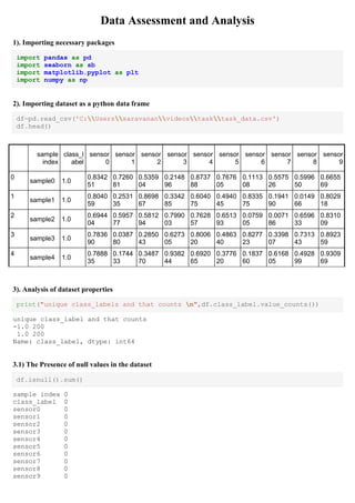
This document analyzes a dataset containing sensor data to evaluate the predictive power of each sensor. It first imports necessary packages and loads the dataset. Various analyses are then performed, including checking for null values, descriptive statistics, and correlation. Two approaches are taken: 1) using log loss to rank the sensors based on predictive accuracy, and 2) using linear discriminant analysis (LDA) to also rank the sensors. Both approaches yield similar results, with sensors 8, 4, and 0 found to be most predictive. Strengths, weaknesses, and scalability of the methods are discussed. Suggestions are made to use log loss due to its optimization properties.

1. Data Assessment and Analysis
1). Importing necessary packages
import pandas as pd
import seaborn as sb
import matplotlib.pyplot as plt
import numpy as np
2). Importing dataset as a python data frame
df=pd.read_csv('C:Userssaravananvideostasktask_data.csv')
df.head()
sample
index
class_l
abel
sensor
0
sensor
1
sensor
2
sensor
3
sensor
4
sensor
5
sensor
6
sensor
7
sensor
8
sensor
9
0
sample0 1.0
0.8342
51
0.7260
81
0.5359
04
0.2148
96
0.8737
88
0.7676
05
0.1113
08
0.5575
26
0.5996
50
0.6655
69
1
sample1 1.0
0.8040
59
0.2531
35
0.8698
67
0.3342
85
0.6040
75
0.4940
45
0.8335
75
0.1941
90
0.0149
66
0.8029
18
2
sample2 1.0
0.6944
04
0.5957
77
0.5812
94
0.7990
03
0.7628
57
0.6513
93
0.0759
05
0.0071
86
0.6596
33
0.8310
09
3
sample3 1.0
0.7836
90
0.0387
80
0.2850
43
0.6273
05
0.8006
20
0.4863
40
0.8277
23
0.3398
07
0.7313
43
0.8923
59
4
sample4 1.0
0.7888
35
0.1744
33
0.3487
70
0.9382
44
0.6920
65
0.3776
20
0.1837
60
0.6168
05
0.4928
99
0.9309
69
3). Analysis of dataset properties
print("unique class_labels and that counts n",df.class_label.value_counts())
unique class_label and that counts
-1.0 200
1.0 200
Name: class_label, dtype: int64
3.1) The Presence of null values in the dataset
df.isnull().sum()
sample index 0
class_label 0
sensor0 0
sensor1 0
sensor2 0
sensor3 0
sensor4 0
sensor5 0
sensor6 0
sensor7 0
sensor8 0
sensor9 0

2. 3.2) Statistical understanding of dataset
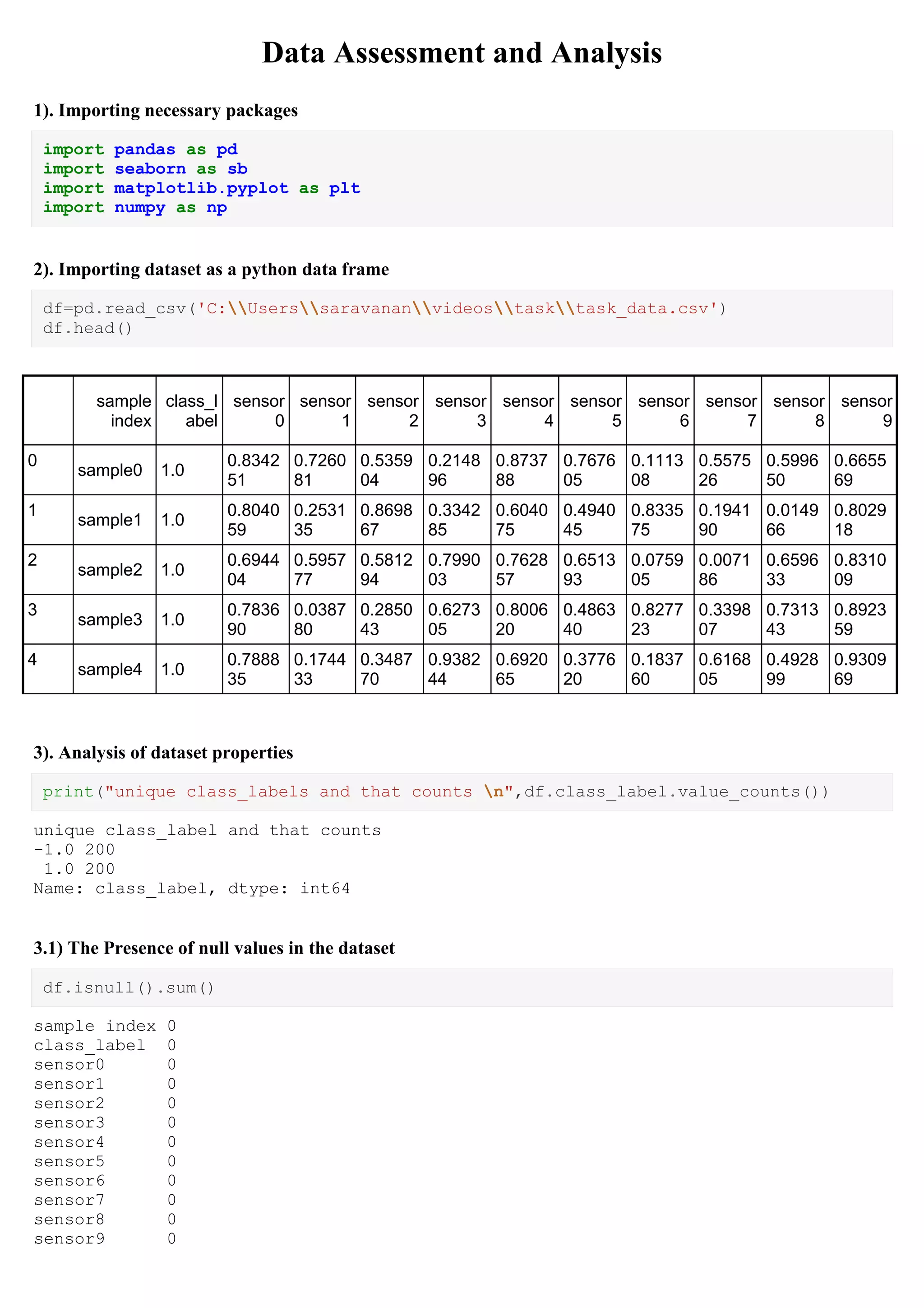
df.describe(include="all")
sampl
e
index
class_l
abel
sensor
0
sensor
1
sensor
2
sensor
3
sensor
4
sensor
5
sensor
6
sensor
7
sensor
8
sensor
9
count
400
400.00
0000
400.00
0000
400.00
0000
400.00
0000
400.00
0000
400.00
0000
400.00
0000
400.00
0000
400.00
0000
400.00
0000
400.00
0000
unique 400 NaN NaN NaN NaN NaN NaN NaN NaN NaN NaN NaN
top sampl
e98
NaN NaN NaN NaN NaN NaN NaN NaN NaN NaN NaN
freq 1 NaN NaN NaN NaN NaN NaN NaN NaN NaN NaN NaN
mean
NaN
0.0000
00
0.5236
61
0.5092
23
0.4812
38
0.5097
52
0.4978
75
0.5010
65
0.4904
80
0.4823
72
0.4828
22
0.5419
33
std
NaN
1.0012
52
0.2681
94
0.2768
78
0.2875
84
0.2977
12
0.2882
08
0.2876
34
0.2899
54
0.2827
14
0.2961
80
0.2724
90
min
NaN
-
1.0000
00
0.0077
75
0.0038
65
0.0044
73
0.0014
66
0.0002
50
0.0004
25
0.0001
73
0.0033
22
0.0031
65
0.0004
52
25%
NaN
-
1.0000
00
0.2997
92
0.2830
04
0.2355
44
0.2626
97
0.2493
69
0.2694
30
0.2266
87
0.2428
48
0.2136
26
0.3212
64
50%
NaN
0.0000
00
0.5349
06
0.5075
83
0.4602
41
0.5100
66
0.4978
42
0.4971
08
0.4773
41
0.4634
38
0.4622
51
0.5783
89
75%
NaN
1.0000
00
0.7518
87
0.7278
43
0.7349
37
0.7689
75
0.7434
01
0.7388
54
0.7353
04
0.7324
83
0.7405
42
0.7689
90
max
NaN
1.0000
00
0.9994
76
0.9986
80
0.9929
63
0.9951
19
0.9994
12
0.9973
67
0.9971
41
0.9982
30
0.9960
98
0.9994
65
3.3) Define Predictor_variables and Target_variable
predictor_variables=df[['sensor0', 'sensor1', 'sensor2','sensor3', 'sensor4',
'sensor5', 'sensor6', 'sensor7', 'sensor8', 'sensor9']]
target_variable=df[['class_label']]
3.4) Variance of predictor_variables data
print("variance of all sensorsnn",np.var(predictor_variables))
variance of all sensors
sensor0 0.071748
sensor1 0.076470
sensor2 0.082498
sensor3 0.088411
sensor4 0.082856
sensor5 0.082527
sensor6 0.083863
sensor7 0.079727
sensor8 0.087503
sensor9 0.074065

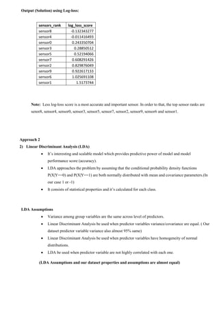
3. 3.5) Probability distributions of the predictor_variables data
sensors=predictor_variables.keys()
for i in range(0,len(predictor_variables.keys())):
k=sensors[i]
sb.distplot(predictor_variables[""+k+""],label=""+k+"",hist=False)
3.6) Correlation analysis of Predictor_variables data
sb.heatmap(predictor_variables.corr())

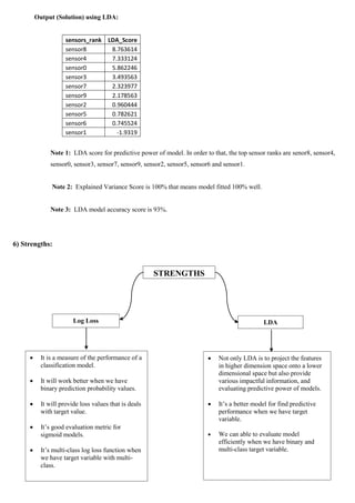
4. 4) Properties of dataset:
1) Our dataset have 12 features with 400 observations.
2) It have one class_label that have either 1 or -1 with each class have equal samples like 200,200.
3) It's don't have any null values.
4) All predictor_variables data start with 0 and end with 1.
5) All predictor_variables data almost 95% normally distributed and also all variables have homogeneity of variance.
6) All predictor_variables are not highly correlated with each one.
5) Assumptions and process of thoughts:
I am going to provide solutions with two approaches.
Approach 1
1) Log loss
Our dataset predictor_variables data start with 0 and end with 1 continuously.
And our class_label (target_variable) have 1 and -1. So, based on those format it’s exactly look like sigmoid
model outputs. If we want to know each sensor performance or predictive power, we can apply log loss metric to
evaluate predictive power of each sensors.
Log loss is the best metrics for binary evolution models / sigmoid function model (logistic or probit
regression) because it will tell the exact loss value of each predicted value. In the sense we can know exact
predictive power of binary model using log loss metric.
Note:
Xi means already predicted values and Y means actual values I derived formula for our problem of case
scenario.
Y = Target_variable (class_label)
Xi …n = Predictor_variables (sensor0, sensor1...n)
n = Number of observations
Log_loss = [(Y * log(Xi)) + ((1-Y) * log(1-X1i))]
Avg_log_loss = [(-1/n)* sum(Log_loss)]

5. Output (Solution) using Log-loss:
sensors_rank log_loss_score
sensor8 -0.132343277
sensor4 -0.011416493
sensor0 0.243350704
sensor3 0.28850512
sensor5 0.52194066
sensor7 0.608291426
sensor2 0.829876049
sensor9 0.922617133
sensor6 1.025691108
sensor1 1.5173744
Note: Less log-loss score is a most accurate and important sensor. In order to that, the top sensor ranks are
senor8, sensor4, sensor0, sensor3, sensor5, sensor7, sensor2, sensor9, sensor6 and sensor1.
Approach 2
2) Linear Discriminant Analysis (LDA)
 It’s interesting and scalable model which provides predictive power of model and model
performance score (accuracy).
 LDA approaches the problem by assuming that the conditional probability density functions
P(X|Y==0) and P(X|Y==1) are both normally distributed with mean and covariance parameters.(In
our case 1 or -1)
 It consists of statistical properties and it’s calculated for each class.
LDA Assumptions
 Variance among group variables are the same across level of predictors.
 Linear Discriminant Analysis be used when predictor variables variance/covariance are equal. ( Our
dataset predictor variable variance also almost 95% same)
 Linear Discriminant Analysis be used when predictor variables have homogeneity of normal
distributions.
 LDA be used when predictor variable are not highly correlated with each one.
(LDA Assumptions and our dataset properties and assumptions are almost equal)

6. Output (Solution) using LDA:
Note 1: LDA score for predictive power of model. In order to that, the top sensor ranks are senor8, sensor4,
sensor0, sensor3, sensor7, sensor9, sensor2, sensor5, sensor6 and sensor1.
Note 2: Explained Variance Score is 100% that means model fitted 100% well.
Note 3: LDA model accuracy score is 93%.
6) Strengths:
sensors_rank LDA_Score
sensor8 8.763614
sensor4 7.333124
sensor0 5.862246
sensor3 3.493563
sensor7 2.323977
sensor9 2.178563
sensor2 0.960444
sensor5 0.782621
sensor6 0.745524
sensor1 -1.9319
STRENGTHS
 It is a measure of the performance of a
classification model.
 It will work better when we have
binary prediction probability values.
 It will provide loss values that is deals
with target value.
 It’s good evaluation metric for
sigmoid models.
 It’s multi-class log loss function when
we have target variable with multi-
class.
 Not only LDA is to project the features
in higher dimension space onto a lower
dimensional space but also provide
various impactful information, and
evaluating predictive power of models.
 It’s a better model for find predictive
performance when we have target
variable.
 We can able to evaluate model
efficiently when we have binary and
multi-class target variable.
Log Loss LDA

7. 7) Weakness:
8) Scalabilities:
WEAKNESS
Log Loss LDA
 Never it’s work when we don’t have
sigmoid value.
 LDA does not work well if the data is
not balanced.
 Sometimes LDA doesn’t work well
when we have too many
observations.
SCALABILITY
Log Loss LDA
 It will provide accurate solution when
we have n dimensional variables and
sample’s
 Doesn’t matter n number of features
and samples because it is working based
mathematical formula.
 Processing time is too low for provide
solution
 We can able to integrate rules (Min-
Max Rule,..) onto it.
 It will work well when we have
multiple number of features.
 Doesn’t matter n number of features in
LDA.
 It will take few seconds to provide
solution that means processing time.

8. 9) Alternative Methods:
1. Threshold Based Scoring Mechanism(TBSM)
Threshold Based Scoring Mechanism is technique which is providing solution based on threshold
score.
Strengths:
 We can provide solution using simple threshold scoring.
 We can optimize threshold values based problem.
Weakness:
 It’s little difficult to provide solution when we have multi-class target variable.
 Difficult to assign threshold values when we have multi-class target variable.
 It will take few more minutes for processing when we have n number features.
 Code modification will happen at all time of processing.
Scalability:
 It not a good method when we have n number of features.
 Modification always there when we going to process new data with same problem.
 It’s not a good scalable method for evaluate model performance and power.
Output (Solution) using TBSM:
sensors_rank Threshold_error_score
sensor8 47
sensor4 66
sensor0 80
sensor3 105
sensor9 182
sensor1 189
sensor7 190
sensor2 197
sensor6 201
sensor5 203
Note 1: Threshold based scoring mechanism scoring of sensors in order to that, the top sensor ranks are
senor8, sensor4, sensor0, sensor3, sensor9, sensor1, sensor7, sensor2, sensor6 and sensor5.

9. 2. Cross- Entropy Error Function:
Cross-entropy error function are slightly different depending on the context, but in machine learning
when calculating error rates between 0 and 1 it’s resolve same like log-loss. But in our case we have
prediction probability
Strengths:
 It’s more like a log-loss function.
 It’s a better loss function in machine learning and optimization.
 It deals with classifying a given set of data points into two possible classes generically labelled 0
and 1 in our case -1 and 1.
 We can able to assign vector of weights W.
 We can use cross entropy to get a measure of dissimilarity between p and q.
Weakness:
 Assigning vector of weights W is fully depends of other optimization modelling like Gradient -
descent.
 Assigning vector of weights W is little difficult when we have multi class target variable.
Scalability:
 We can perform efficiently when we have n number features because it’s also a mathematical
formula directly applied on problem.
10) Suggestions:
 LDA and log-loss providing 90% same solution.
 Log-loss is more popular and optimization loss function which provide exact loss value
for each observation deals with target observation. So, it’s a good approach for this
model evaluation task.
 Linear Discriminant Analysis is interesting and new approach for evaluate model
predictive power which will tell most accurate prediction variable (sensor).
 We can do further optimizing techniques, modelling, pipelines using this both.
Y = Target_variable (class_label)
Xi …n = Predictor_variables (sensor0, sensor1...n)
p = {Y, 1-Y}
q = {Xi, 1-Xi}
H (p, q) = -Y log Xi – (1- Y) log (1-Xi)