The document is a comprehensive guide to DAX (Data Analysis Expressions), authored by Marco Russo and Alberto Ferrari, focusing on business intelligence using Microsoft tools such as Excel and Power BI. It covers various topics, including basic and advanced functionalities of DAX, time intelligence calculations, table functions, and optimization techniques. The book serves as a definitive resource for both beginners and experienced users looking to enhance their understanding of DAX in data analysis contexts.


![62 The Definitive Guide to DAX
Introduction to evaluation contexts
Let’s begin by understanding what an evaluation context is. Any DAX expression is evaluated inside
a context. The context is the “environment” under which the formula is evaluated. For example,
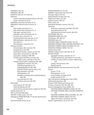
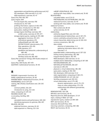
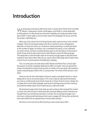
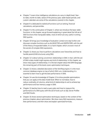
consider a very simple formula for a measure such as:
[Sales Amount] := SUMX ( Sales, Sales[Quantity] * Sales[UnitPrice] )
You already know what this formula computes: the sum of all the values of quantity multiplied by
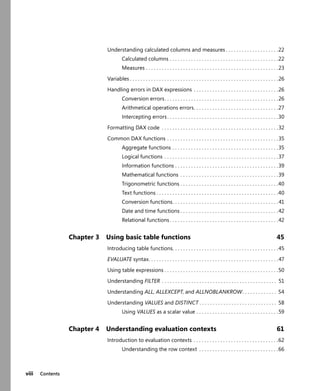
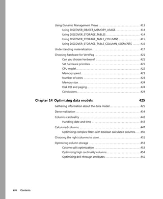
price in the Sales table. You can put this measure in a pivot table and look at the results, as you can
see in Figure 4-1.
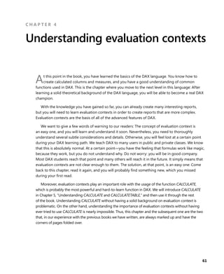
FIGURE 4-1 The measure Sales Amount, without a context, shows the grand total of sales.
Well, this number alone does not look interesting at all, does it? But, if you think carefully, the
formula computes exactly what it is supposed to compute: the sum of all sales amount, which is a
big number with no interesting meaning. This pivot table becomes more interesting as soon as we
use some columns to slice the grand total and start investigating it. For example, you can take the
product color, put it on the rows, and the pivot table suddenly reveals some interesting business
insights, as you can see in Figure 4-2.
The grand total is still there, but now it is the sum of smaller values and each value, together with
all the others, has a meaning. However, if you think carefully again, you should note that something
weird is happening here: the formula is not computing what we asked.
We supposed that the formula meant “the sum of all sales amount.” but inside each cell of the
pivot table, the formula is not computing the sum of all sales, it is only computing the sum of sales of
products with a specific color. Yet, we never specified that the computation had to work on a subset
of the data model. In other words, the formula does not specify that it can work on subsets of data.
Why is the formula computing different values in different cells? The answer is very easy, indeed:
because of the evaluation context under which DAX computes the formula. You can think of the
evaluation context of a formula as the surrounding area of the cell where DAX evaluates the formula.
[Sales Amount] := SUMX ( Sales, Sales[Quantity] * Sales[UnitPrice] )](https://image.slidesharecdn.com/librodaxbi-240516004012-1966db37/85/Formulas-dax-para-power-bI-de-microsoft-pdf-29-320.jpg)
![CHAPTER 4 Understanding evaluation contexts 65
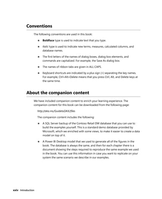
Each cell has a different value because there are two fields on the rows, color and brand name. The
complete set of fields on rows and columns defines the context. For example, the context of the cell
highlighted in Figure 4-4 corresponds to color Black, brand Contoso, and Calendar Year 2007.
Note It is not important whether a field is on the rows or on the columns (or on the slicer
and/or page filter, or in any other kind of filter you can create with a query). All of these
filters contribute to define a single context, which DAX uses to evaluate the formula.
Putting a field on rows or columns has just some aesthetic consequences, but nothing
changes in the way DAX computes values.
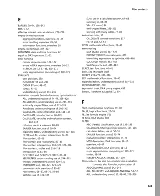
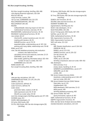
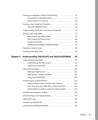
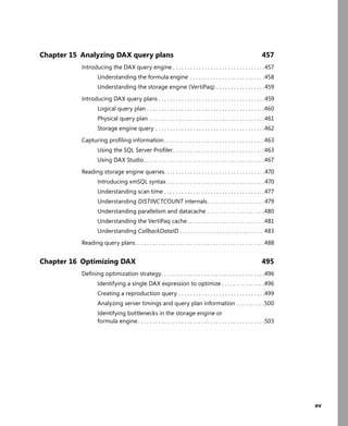
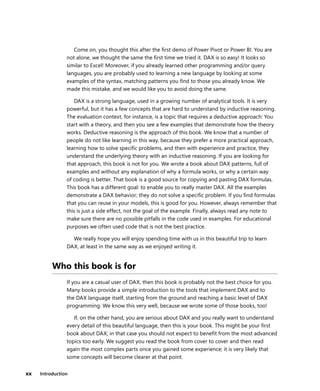
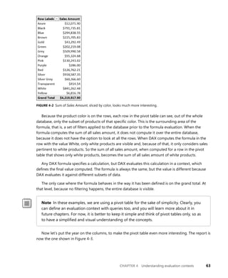
Let’s see the full picture now. In Figure 4-5, we added the product category on a slicer, and the
month name on a filter, where we selected December.
FIGURE 4-5 In a typical report, the context is defined in many ways, including slicers and filters.
It is clear at this point that the values computed in each cell have a context defined by rows,
columns, slicers, and filters. All these filters contribute in the definition of a context that DAX applies
to the data model prior to the formula evaluation. Moreover, it is important to learn that not all the
cells have the same set of filters, not only in terms of values, but also in terms of fields. For example,
the grand total on the columns contains only the filter for category, month, and year, but it does not
contain the filter for color and brand. The fields for color and brand are on the rows and they do not
filter the grand total. The same applies to the subtotal by color within the pivot table: for those cells
there is no filter on the manufacturer, the only valid filter coming from the rows is the color.
We call this context the Filter Context and, as its name suggests, it is a context that filters tables.
Any formula you ever author will have a different value depending on the filter context that DAX uses
to perform its evaluation. This behavior, although very intuitive, needs to be well understood.
Now that you have learned what a filter context is, you know that the following DAX expression
should be read as “the sum of all sales amount visible in the current filter context”:
[Sales Amount] := SUMX ( Sales, Sales[Quantity] * Sales[UnitPrice] )
[Sales Amount] := SUMX ( Sales, Sales[Quantity] * Sales[UnitPrice] )](https://image.slidesharecdn.com/librodaxbi-240516004012-1966db37/85/Formulas-dax-para-power-bI-de-microsoft-pdf-32-320.jpg)
![66 The Definitive Guide to DAX
You will learn later how to read, modify, and clear the filter context. As of now, it is enough having
a solid understanding of the fact that the filter context is always present for any cell of the pivot table
or any value in your report/query. You always need to take into account the filter context in order to
understand how DAX evaluates a formula.
Understanding the row context
The filter context is one of the two contexts that exist in DAX. Its companion is the row context and, in
this section, you will learn what it is and how it works.
This time, we use a different formula for our considerations:
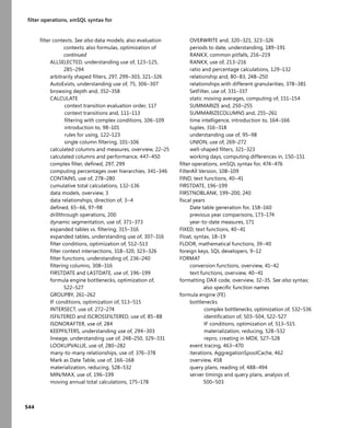
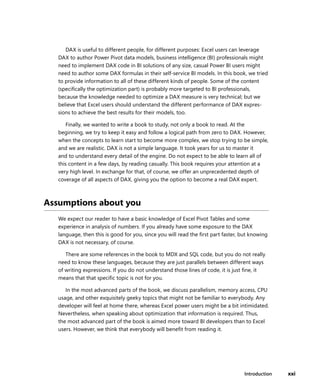
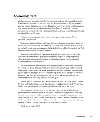
Sales[GrossMargin] = Sales[SalesAmount] - Sales[TotalCost]
You are likely to write such an expression in a calculated column, in order to compute the gross
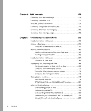
margin. As soon as you define this formula in a calculated column, you will get the resulting table, as
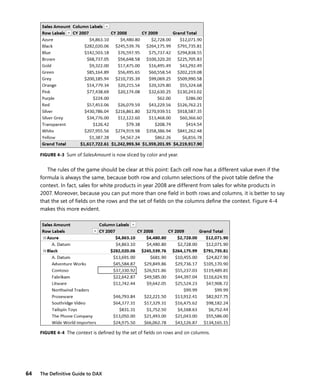
shown in Figure 4-6.
FIGURE 4-6 The GrossMargin is computed for all the rows of the table.
DAX computed the formula for all the rows of the table and, for each row, it computed a different
value, as expected. In order to understand the row context, we need to be somewhat pedantic in our
reading of the formula: we asked to subtract two columns, but where did we tell DAX from which row
of the table to get the values of the columns? You might say that the row to use is implicit. Because it
is a calculated column, DAX computes it row by row and, for each row, it evaluates a different result.
This is correct, but, from the point of view of the DAX expression, the information about which row to
use is still missing.
In fact, the row used to perform a calculation is not stored inside the formula. It is defined by
another kind of context: the row context. When you defined the calculated column, DAX started an
iteration from the first row of the table; it created a row context containing that row and evaluated
the expression. Then it moved on to the second row and evaluated the expression again. This
happens for all the rows in the table and, if you have one million rows, you can think that DAX created
one million row contexts to evaluate the formula one million times. Clearly, in order to optimize
calculations, this is not exactly what happens; otherwise, DAX would be a very slow language. Anyway,
from the logical point of view, this is exactly how it works.
Sales[GrossMargin] = Sales[SalesAmount] - Sales[TotalCost]](https://image.slidesharecdn.com/librodaxbi-240516004012-1966db37/85/Formulas-dax-para-power-bI-de-microsoft-pdf-33-320.jpg)
![CHAPTER 4 Understanding evaluation contexts 67
Let us try to be more precise. A row context is a context that always contains a single row and DAX
automatically defines it during the creation of calculated columns. You can create a row context using
other techniques, which are discussed later in this chapter, but the easiest way to explain row context
is to look at calculated columns, where the engine always creates it automatically.
There are always two contexts
So far, you have learned what the row context and the filter context are. They are the only kind
of contexts in DAX. Thus, they are the only way to modify the result of a formula. Any formula
will be evaluated under these two distinct contexts: the row context and the filter context.
We call both contexts “evaluation contexts,” because they are contexts that change the way
a formula is evaluated, providing different results for the same formula.
This is one point that is very important and very hard to focus on at the beginning: there
are always two contexts and the result of a formula depends on both. At this point of your DAX
learning path, you probably think that this is obvious and very natural. You are probably right.
However, later in the book, you will find formulas that will be a challenge to understand if you
do not remember about the coexistence of the two contexts, each of which can change the
result of the formula.
Testing your evaluation context understanding
Before we move on with more complex discussions about evaluation contexts, we would like to test
your understanding of contexts with a couple of examples. Please do not look at the explanation
immediately; stop after the question and try to answer it. Then read the explanation to make sense
out of it.
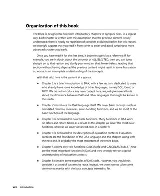
Using SUM in a calculated column
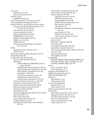
The first test is a very simple one. What is happening if you define a calculated column, in Sales, with
this code?
Sales[SumOfSalesAmount] = SUM ( Sales[SalesAmount] )
Because it is a calculated column, it will be computed row by row and, for each row, you will obtain
a result. What number do you expect to see? Choose one from among these options:
■ The value of SalesAmount for that row, that is, a different value for each row.
■ The total of SalesAmount for all the rows, that is, the same value for all the rows.
■ An error; you cannot use SUM inside a calculated column.
Sales[SumOfSalesAmount] = SUM ( Sales[SalesAmount] )](https://image.slidesharecdn.com/librodaxbi-240516004012-1966db37/85/Formulas-dax-para-power-bI-de-microsoft-pdf-34-320.jpg)
![68 The Definitive Guide to DAX
Stop reading, please, while we wait for your educated guess before moving on.
Now, let’s elaborate on what is happening when DAX evaluates the formula. You already learned
what the formula meaning is: “the sum of all sales amount as seen in the current filter context.” As
this is in a calculated column, DAX evaluates the formula row by row. Thus, it creates a row context
for the first row, and then invokes the formula evaluation and proceeds iterating the entire table. The
formula computes the sum of all sales amount values in the current filter context, so the real question
is “What is the current filter context?” Answer: It is the full database, because DAX evaluates the
formula outside of any pivot table or any other kind of filtering. In fact, DAX computes it as part of
the definition of a calculated column, when no filter is active.
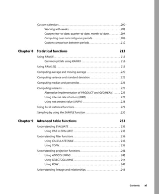
Even if there is a row context, SUM ignores it. Instead, it uses the filter context and the filter
context right now is the full database. Thus, the second option is correct: You will get the grand total
of sales amount, the same value for all the rows of Sales, as you can see in Figure 4-7.
FIGURE 4-7 SUM ( Sales[SalesAmount] ), in a calculated column, is computed against the full database.
This example shows that the two contexts exist together. They both work on the result of a
formula, but in different ways. Aggregate functions like SUM, MIN, and MAX used in calculated
columns use the filter context only and ignore the row context, which DAX uses only to determine
column values. If you have chosen the first answer, as many students typically do, it is perfectly
normal. The point is that you are not yet thinking that the two contexts are working together to
change the formula result in different ways. The first answer is the most common, when using
intuitive logic, but it is the wrong one, and now you know why.
Using columns in a measure
The second test we want to do with you is slightly different. Imagine you want to define the formula
for gross margin in a measure instead of in a calculated column. You have a column with the sales
amount, another column for the product cost, and you might write the following expression:](https://image.slidesharecdn.com/librodaxbi-240516004012-1966db37/85/Formulas-dax-para-power-bI-de-microsoft-pdf-35-320.jpg)
![CHAPTER 4 Understanding evaluation contexts 69
[GrossMargin] := Sales[SalesAmount] - Sales[ProductCost]
What result should you expect if you try to author such a measure?
1. The expression works correctly, we will need to test the result in a report.
2. An error, you cannot even author this formula.
3. You can define the formula, but it will give an error when used in a pivot table or in a query.
As before, stop reading, think about the answer, and then read the following explanation.
In the formula, we used Sales[SalesAmount], which is a column name, that is, the value of
SalesAmount in the Sales table. Is this definition lacking something? You should recall, from previ-
ous arguments, that the information missing here is the row from where to get the current value of
SalesAmount. When you write this code inside a calculated column, DAX knows the row to use when
it computes the expression, thanks to the row context. However, what happens for a measure? There
is no iteration, there is no current row, that is, there is no row context.
Thus, the second answer is correct. You cannot even write the formula; it is syntactically wrong and
you will receive an error when you try to enter it.
Remember that a column does not have a value by itself. Instead, it has a different value for each
row of a table. Thus, if you want a single value, you need to specify the row to use. The only way to
specify the row to use is the row context. Because inside this measure there is no row context, the
formula is incorrect and DAX will refuse it.
The correct way to specify this calculation in a measure is to use aggregate functions, as in:
[GrossMargin] := SUM ( Sales[SalesAmount] ) - SUM ( Sales[ProductCost] )
Using this formula, you are now asking for an aggregation through SUM. Therefore, this latter
formula does not depend on a row context; it only requires a filter context and it provides the correct
result.
Creating a row context with iterators
You learned that DAX automatically creates a row context when you define a calculated column. In
that case, the engine evaluates the DAX expression on a row-by-row basis. Now, it is time to learn
how to create a row context inside a DAX expression by using iterators.
You might recall from Chapter 2, “Introducing DAX,” that all the X-ending functions are iterators,
that is, they iterate over a table and evaluate an expression for each row, finally aggregating the
results using different algorithms. For example, look at the following DAX expression:
[GrossMargin] := Sales[SalesAmount] - Sales[ProductCost]
[GrossMargin] := SUM ( Sales[SalesAmount] ) - SUM ( Sales[ProductCost] )](https://image.slidesharecdn.com/librodaxbi-240516004012-1966db37/85/Formulas-dax-para-power-bI-de-microsoft-pdf-36-320.jpg)
![70 The Definitive Guide to DAX
[IncreasedSales] := SUMX ( Sales, Sales[SalesAmount] * 1.1 )
SUMX is an iterator, it iterates the Sales table and, for each row of the table, it evaluates the
sales amount adding 10 percent to its value, finally returning the sum of all these values. In order
to evaluate the expression for each row, SUMX creates a row context on the Sales table and uses it
during the iteration. DAX evaluates the inner expression (the second parameter of SUMX) in a row
context containing the currently iterated row.
It is important to note that different parameters of SUMX use different contexts during the full
evaluation flow. Let’s look closer at the same expression:
= SUMX (
Sales, External contexts
Sales[SalesAmount] * 1.1 External contexts + new Row Context
)
The first parameter, Sales, is evaluated using the context coming from the caller (for example, it
might be a pivot table cell, another measure, or part of a query), whereas the second parameter (the
expression) is evaluated using both the external context plus the newly created row context.
All iterators behave in the same way:
1. Create a new row context for each row of the table received as the first parameter.
2. Evaluate the second parameter inside the newly created row context (plus any other context
which existed before the iteration started), for each row of the table.
3. Aggregate the values computed during step 2.
It is important to remember that the original contexts are still valid inside the expression: Iterators
only add a new row context; they do not modify existing ones in any way. This rule is usually valid, but
there is an important exception: If the previous contexts already contained a row context for the same
table, then the newly created row context hides the previously existing row context. We are going to
discuss this in more detail in the next section.
Using the EARLIER function
The scenario of having many nested row contexts on the same table might seem very rare, but, in
reality, it happens quite often. Let’s see the concept with an example. Imagine you want to count, for
each product, the number of other products with a higher price. This will produce a sort of ranking of
the product based on price.
To solve this exercise, we use the FILTER function, which you learned in the previous chapter. As
you might recall, FILTER is an iterator that loops through all the rows of a table and returns a new
[IncreasedSales] := SUMX ( Sales, Sales[SalesAmount] * 1.1 )
= SUMX (
Sales, External contexts
Sales[SalesAmount] * 1.1 External contexts + new Row Context
)](https://image.slidesharecdn.com/librodaxbi-240516004012-1966db37/85/Formulas-dax-para-power-bI-de-microsoft-pdf-37-320.jpg)
![CHAPTER 4 Understanding evaluation contexts 71
table containing only the ones that satisfy the condition defined by the second parameter. For
example, if you want to retrieve the table of products with a price higher than US$100, you can use:
= FILTER ( Product, Product[UnitPrice] > 100 )
Note The careful reader will have noted that FILTER needs to be an iterator because the
expression Product[UnitPrice]>100 can be evaluated if and only if a valid row context exists
for Product; otherwise the effective value of Unit Price would be indeterminate. FILTER
is an iterator function that creates a row context for each row of the table in the first
argument, which makes it possible to evaluate the condition in the second argument.
Now, let’s go back to our original example: creating a calculated column that counts the number
of products that have a higher price than the current one. If you would name the price of the current
product PriceOfCurrentProduct, then it is easy to see that this pseudo-DAX formula would do what
is needed:
Product[UnitPriceRank] =
COUNTROWS (
FILTER (
Product,
Product[UnitPrice] > PriceOfCurrentProduct
)
)
FILTER returns only the products with a price higher than the current one and COUNTROWS
counts those products. The only remaining issue is a way to express the price of the current product,
replacing PriceOfCurrentProduct with a valid DAX syntax. With “current,” we mean the value of the
column in the current row when DAX computes the column. It is harder than you might expect.
You define this new calculated column inside the Product table. Thus, DAX evaluates the
expression inside a row context. However, the expression uses a FILTER that creates a new row context
on the same table. In fact, Product[UnitPrice] used in the fifth row of the previous expression is the
value of the unit price for the current row iterated by FILTER - our inner iteration. Therefore, this
new row context hides the original row context introduced by the calculated column. Do you see
the issue? You want to access the current value of the unit price but not use the last introduced row
context. Instead, you want to use the previous row context, that is, the one of the calculated column.
DAX provides a function that makes it possible: EARLIER. EARLIER retrieves the value of a
column by using the previous row context instead of the last one. So you can express the value of
PriceOfCurrentProduct using EARLIER(Product[UnitPrice]).
EARLIER is one of the strangest functions in DAX. Many users feel intimidated by EARLIER, because
they do not think in terms of row contexts and they do not take into account the fact that you can
= FILTER ( Product, Product[UnitPrice] > 100 )
Product[UnitPriceRank] =
COUNTROWS (
FILTER (
Product,
Product[UnitPrice] > PriceOfCurrentProduct
)
)](https://image.slidesharecdn.com/librodaxbi-240516004012-1966db37/85/Formulas-dax-para-power-bI-de-microsoft-pdf-38-320.jpg)
![72 The Definitive Guide to DAX
nest row contexts by creating multiple iterations over the same table. In reality, EARLIER is a very
simple function that will be useful many times. The following code finally solves the scenario:
Product[UnitPriceRank] =
COUNTROWS (
FILTER (
Product,
Product[UnitPrice] > EARLIER ( Product[UnitPrice] )
)
) + 1
In Figure 4-8 you can see the calculated column defined in the Product table, which has been
sorted using Unit Price in a descending order.
FIGURE 4-8 UnitPriceRank is a useful example of how EARLIER is useful to navigate in nested row contexts.
Because there are fourteen products with the same unit price, their rank is always one; the
fifteenth product has a rank of 15, shared with other products with the same price. We suggest you
study and understand this small example closely, because it is a very good test to check your ability to
use and understand row contexts, how to create them using iterators (FILTER, in this case), and how to
access values outside of them through the usage of EARLIER.
Note EARLIER accepts a second parameter, which is the number of steps to skip, so that you
can skip two or more row contexts. Moreover, there is also a function named EARLIEST that
lets you access directly the outermost row context defined for a table. To be honest, neither
the second parameter of EARLIER nor EARLIEST is used often: while having two nested row
contexts is a common scenario, having three or more of them is something that happens rarely.
Product[UnitPriceRank] =
COUNTROWS (
FILTER (
Product,
Product[UnitPrice] > EARLIER ( Product[UnitPrice] )
)
) + 1](https://image.slidesharecdn.com/librodaxbi-240516004012-1966db37/85/Formulas-dax-para-power-bI-de-microsoft-pdf-39-320.jpg)
![CHAPTER 4 Understanding evaluation contexts 73
Before leaving this example, it is worth noting that, if you want to transform this value into a
better ranking (that is, a value that starts with 1 and grows of one, creating a sequence 1, 2, 3…) then
counting the prices instead of counting the products is sufficient. Here, the VALUES function, which
you learned in the previous chapter, comes to help:
Product[UnitPriceRankDense] =
COUNTROWS (
FILTER (
VALUES ( Product[UnitPrice] ),
Product[UnitPrice] > EARLIER ( Product[UnitPrice] )
)
) + 1
In Figure 4-9 you can see the new calculated column.
FIGURE 4-9 UnitPriceRankDense shows a better ranking, because it counts the prices, not the products.
We strongly suggest you learn and understand EARLIER thoroughly, because you will use it very
often. Nevertheless, it is important to note that variables can be used—in many scenarios—to avoid
the use of EARLIER. Moreover, a careful use of variables makes the code much easier to read. For
example, you can compute the previous calculated column using this expression:
Product[UnitPriceRankDense] =
VAR
CurrentPrice = Product[UnitPrice]
RETURN
COUNTROWS (
FILTER (
VALUES ( Product[UnitPrice] ),
Product[UnitPrice] > CurrentPrice
)
) + 1
Product[UnitPriceRankDense] =
COUNTROWS (
FILTER (
VALUES ( Product[UnitPrice] ),
Product[UnitPrice] > EARLIER ( Product[UnitPrice] )
)
) + 1
Product[UnitPriceRankDense] =
VAR
CurrentPrice = Product[UnitPrice]
RETURN
COUNTROWS (
FILTER (
VALUES ( Product[UnitPrice] ),
Product[UnitPrice] > CurrentPrice
)
) + 1](https://image.slidesharecdn.com/librodaxbi-240516004012-1966db37/85/Formulas-dax-para-power-bI-de-microsoft-pdf-40-320.jpg)
![74 The Definitive Guide to DAX
In this final example, using a variable, you store the current unit price in the CurrentPrice variable,
which you use later to perform the comparison. Giving a name to the variable, you make the
code easier to read, without having to traverse the stack of row contexts every time you read the
expression to make sense of the evaluation flow.
Understanding FILTER, ALL, and context interactions
In the preceding example, we have used FILTER as a convenient way of filtering a table. FILTER is a very
common function to use, whenever you want to apply a filter that further restricts the existing context.
Imagine that you want to create a measure that counts the number of red products. With the
knowledge you gained so far, the formula is an easy one:
[NumOfRedProducts] :=
COUNTROWS (
FILTER (
Product,
Product[Color] = "Red"
)
)
This formula works fine and you can use it inside a pivot table; for example, putting the brand on
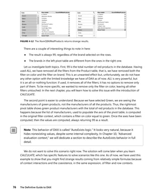
the rows to produce the report shown in Figure 4-10.
FIGURE 4-10 You can easily count the number of red products using the FILTER function.
Before moving on with this example, it is useful to stop for a moment and think carefully how
DAX computed these values. The brand is a column of the Product table. The engine evaluates
NumOfRedProducts inside each cell, in a context defined by the brand on the rows. Thus, each cell
shows the number of red products that also have the brand indicated by the corresponding row.
This happens because, when you ask to iterate over the Product table, you are really asking to iterate
the Product table as it is visible in the current filter context, which contains only products with that
specific brand. It might seem trivial, but it is better to remember it multiple times than take a chance
of forgetting it.
[NumOfRedProducts] :=
COUNTROWS (
FILTER (
Product,
Product[Color] = "Red"
)
)](https://image.slidesharecdn.com/librodaxbi-240516004012-1966db37/85/Formulas-dax-para-power-bI-de-microsoft-pdf-41-320.jpg)
![CHAPTER 4 Understanding evaluation contexts 75
This is more evident if you put a slicer on the worksheet containing the color. In Figure 4-11 we
have created two identical pivot tables with the slicer on color. You can see that the left one has the
color Red selected, and the numbers are the same as in Figure 4-10, whereas in the right one the
pivot table is empty because the slicer has the color Green selected.
FIGURE 4-11 DAX evaluates NumOfRedProducts taking into account the outer context defined by the slicer.
In the right pivot table, the Product table passed into FILTER contains only Green products and,
because there are no products that can be red and green at the same time, it always evaluates to
BLANK (that is, FILTER does not return any row that COUNTROWS can work on).
The important part of this example is the fact that, in the same formula, there are both a filter
context coming from the outside (the pivot table cell, which is affected by the slicer selection) and a
row context introduced in the formula. Both contexts work at the same time and modify the formula
result. DAX uses the filter context to evaluate the Product table, and the row context to filter rows
during the iteration.
At this point, you might want to define another formula that returns the number of red products
regardless of the selection done on the slicer. Thus, you want to ignore the selection made on the
slicer and always return the number of the red products.
You can easily do this by using the ALL function. ALL returns the content of a table ignoring the
filter context, that is, it always returns all the rows of a table. You can define a new measure, named
NumOfAllRedProducts, by using this expression:
[NumOfAllRedProducts] :=
COUNTROWS (
FILTER (
ALL ( Product ),
Product[Color] = "Red"
)
)
This time, instead of referring to Product only, we use ALL ( Product ), meaning that we want to
ignore the existing filter context and always iterate over all products. The result is definitely not what
we would expect, as you can see in Figure 4-12.
[NumOfAllRedProducts] :=
COUNTROWS (
FILTER (
ALL ( Product ),
Product[Color] = "Red"
)
)](https://image.slidesharecdn.com/librodaxbi-240516004012-1966db37/85/Formulas-dax-para-power-bI-de-microsoft-pdf-42-320.jpg)
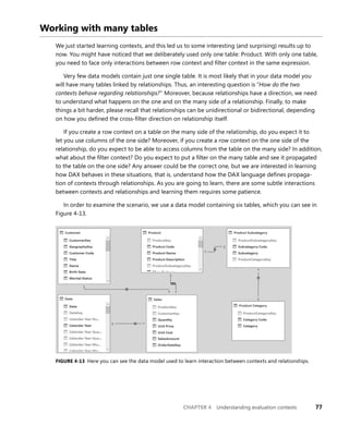
![78 The Definitive Guide to DAX
There are a couple of things to note about this model:
■ There is a chain of one-to-many relationships starting from Sales and reaching Product
Category, through Product and Product Subcategory.
■ The only bidirectional relationship is the one between Sales and Product. All remaining rela-
tionships are set to be one-way cross-filter direction.
Now that we have defined the model, let’s start looking at how the contexts behave by looking at
some DAX formulas.
Row contexts and relationships
The interaction of row contexts and relationships is very easy to understand, because there is nothing
to understand: they do not interact in any way, at least not automatically.
Imagine you want to create a calculated column in the Sales table containing the difference
between the unit price stored in the fact table and the product list price stored in the Product table.
You could try this formula:
Sales[UnitPriceVariance] = Sales[UnitPrice] - Product[UnitPrice]
This expression uses two columns from two different tables and DAX evaluates it in a row context
that iterates over Sales only, because you defined the calculated column within that table (Sales).
Product is on the one side of a relationship with Sales (which is on the many side), so you might
expect to be able to gain access to the unit price of the related row (the product sold). Unfortunately,
this does not happen. The row context in Sales does not propagate automatically to Product and DAX
returns an error if you try to create a calculated column by using the previous formula.
If you want to access columns on the one side of a relationship from the table on the many side of
the relationship, as is the case in this example, you must use the RELATED function. RELATED accepts
a column name as the parameter and retrieves the value of the column in a corresponding row that is
found by following one or more relationships in the many-to-one direction, starting from the current
row context.
You can correct the previous formula with the following code:
Sales[UnitPriceVariance] = Sales[UnitPrice] - RELATED ( Product[UnitPrice] )
RELATED works when you have a row context on the table on the many side of a relationship.
If the row context is active on the one side of a relationship, then you cannot use it because many
rows would potentially be detected by following the relationship. In this case, you need to use
RELATEDTABLE, which is the companion of RELATED. You can use RELATEDTABLE on the one side of
the relationship and it returns all the rows (of the table on the many side) that are related with the
Sales[UnitPriceVariance] = Sales[UnitPrice] - Product[UnitPrice]
Sales[UnitPriceVariance] = Sales[UnitPrice] - RELATED ( Product[UnitPrice] )](https://image.slidesharecdn.com/librodaxbi-240516004012-1966db37/85/Formulas-dax-para-power-bI-de-microsoft-pdf-45-320.jpg)
![CHAPTER 4 Understanding evaluation contexts 79
current one. For example, if you want to compute the number of sales of each product, you can use
the following formula, defined as a calculated column on Product:
Product[NumberOfSales] = COUNTROWS ( RELATEDTABLE ( Sales ) )
This expression counts the number of rows in the Sales table that correspond to the current
product. You can see the result in Figure 4-14.
FIGURE 4-14 RELATEDTABLE is very useful when you have a row context on the one side of the relationship.
It is worth noting that both, RELATED and RELATEDTABLE, can traverse a long chain of relation-
ships to gather their result; they are not limited to a single hop. For example, you can create a column
with the same code as before but, this time, in the Product Category table:
'Product Category'[NumberOfSales] = COUNTROWS ( RELATEDTABLE ( Sales ) )
The result is the number of sales for the category, which traverses the chain of relationships from
Product Category to Product Subcategory, then to Product to finally reach the Sales table.
Note The only exception to the general rule of RELATED and RELATEDTABLE is for one-
to-one relationships. If two tables share a 1:1 relationship, then you can use both RELATED
and RELATEDTABLE in both tables and you will get as a result either a column value or a
table with a single row, depending on the function you have used.
The only limitation—with regards to chains of relationships—is that all the relationships need to be
of the same type (that is, one-to-many or many-to-one), and all of them going in the same direction.
If you have two tables related through one-to-many and then many-to-one, with an intermediate
bridge table in the middle, then neither RELATED nor RELATEDTABLE will work. A 1:1 relationship be-
haves at the same time as a one-to-many and as a many-to-one. Thus, you can have a 1:1 relationship
in a chain of one-to-many without interrupting the chain.
Product[NumberOfSales] = COUNTROWS ( RELATEDTABLE ( Sales ) )
'Product Category'[NumberOfSales] = COUNTROWS ( RELATEDTABLE ( Sales ) )](https://image.slidesharecdn.com/librodaxbi-240516004012-1966db37/85/Formulas-dax-para-power-bI-de-microsoft-pdf-46-320.jpg)
![80 The Definitive Guide to DAX
Let’s make this concept clearer with an example. You might think that Customer is related with
Product because there is a one-to-many relationship between Customer and Sales, and then a many-
to-one relationship between Sales and Product. Thus, a chain of relationships links the two tables.
Nevertheless, the two relationships are not in the same direction.
We call this scenario a many-to-many relationship. In other words, a customer is related to many
products (the ones bought) and a product is related to many customers (the ones who bought the
product). You will learn the details of how to make many-to-many relationships work later; let’s focus
on row context, for the moment. If you try to apply RELATEDTABLE through a many-to-many relation-
ship, the result could be not what you might expect. For example, consider a calculated column in
Product with this formula:
Product[NumOfBuyingCustomers] = COUNTROWS ( RELATEDTABLE ( Customer ) )
You might expect to see, for each row, the number of customers who bought that product.
Unexpectedly, the result will always be 18869, that is, the total number of customers in the database,
as you can see in Figure 4-15.
FIGURE 4-15 RELATEDTABLE does not work if you try to traverse a many-to-many relationship.
RELATEDTABLE cannot follow the chain of relationships because they are not in the same direction:
one is one-to-many, the other one is many-to-one. Thus, the filter from Product cannot reach
Customers. It is worth noting that if you try the formula in the opposite direction, that is, you count,
for each of the customers, the number of bought products, the result will be correct: a different
number for each row representing the number of products bought by the customer. The reason for
this behavior is not the propagation of a filter context but, rather, the context transition created by a
hidden CALCULATE inside RELATEDTABLE. We added this final note for the sake of completeness. It is
not yet time to elaborate on this: You will have a better understanding of this after reading Chapter 5,
“Understanding CALCULATE and CALCULATETABLE.”
Filter context and relationships
You have learned that row context does not interact with relationships and that, if you want to
traverse relationships, you have two different functions to use, depending on which side of the
relationship you are on while accessing the target table.
Product[NumOfBuyingCustomers] = COUNTROWS ( RELATEDTABLE ( Customer ) )](https://image.slidesharecdn.com/librodaxbi-240516004012-1966db37/85/Formulas-dax-para-power-bI-de-microsoft-pdf-47-320.jpg)
![CHAPTER 4 Understanding evaluation contexts 81
Filter contexts behave in a different way: They interact with relationships in an automatic way and
they have different behaviors depending on how you set the filtering of the relationship. The general
rule is that the filter context propagates through a relationship if the filtering direction set on the
relationship itself makes propagation feasible.
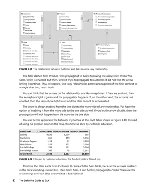
This behavior is very easy to understand by using a simple pivot table with a few measures. In
Figure 4-16 you can see a pivot table browsing the data model we have used so far, with three very
simple measures defined as follows:
[NumOfSales] := COUNTROWS ( Sales )
[NumOfProducts] := COUNTROWS ( Product )
[NumOfCustomers] := COUNTROWS ( Customer )
FIGURE 4-16 Here you can see the behavior of filter context and relationships.
The filter is on the product color. Product is the source of a one-to-many relationship with Sales,
so the filter context propagates from Product to Sales, and you can see this because the NumOfSales
measure counts only the sales of products with the specific color. NumOfProducts shows the number
of products of each color, and a different value for each row (color) is what you would expect,
because the filter is on the same table where we are counting.
On the other hand, NumOfCustomers, which counts the number of customers, always shows the
same value, that is, the total number of customers. This is because the relationship between Customer
and Sales, as you can see Figure 4-17, has an arrow in the direction of Sales.
[NumOfSales] := COUNTROWS ( Sales )
[NumOfProducts] := COUNTROWS ( Product )
[NumOfCustomers] := COUNTROWS ( Customer )](https://image.slidesharecdn.com/librodaxbi-240516004012-1966db37/85/Formulas-dax-para-power-bI-de-microsoft-pdf-48-320.jpg)
![84 The Definitive Guide to DAX
Introducing VALUES
The previous example is very interesting, because it shows how to compute the number of customers
who bought a product by using the direction of filtering. Nevertheless, if you are interested only
in counting the number of customers, then there is an interesting alternative that we take as an
opportunity to introduce as another powerful function: VALUES.
VALUES is a table function that returns a table of one column only, containing all the values of a
column currently visible in the filter context. There are many advanced uses of VALUES, which we will
introduce later. As of now, it is helpful to start using VALUES just to be acquainted with its behavior.
In the previous pivot table, you can modify the definition of NumOfCustomers with the following
DAX expression:
[NumOfCustomers] := COUNTROWS ( VALUES ( Sales[CustomerKey] ) )
This expression does not count the number of customers in the Customer table. Instead, it counts
the number of values visible in the current filter context for the CustomerKey column in Sales. Thus,
the expression does not depend on the relationship between Sales and Customers; it uses only the
Sales table.
When you put a filter on Products, it also always filters Sales, because of the propagation of the
filter from Product to Sales. Therefore, not all the values of CustomerKey will be visible, but only the
ones present in rows corresponding to sales of the filtered products.
The meaning of the expression is “count the number of customer keys for the sales related to the
selected products.” Because a customer key represents a customer, the expression effectively counts
the number of customers who bought those products.
Note You can achieve the same result using DISTINCTCOUNT, which counts the number
of distinct values of a column. As a general rule, it is better to use DISTINCTCOUNT than
COUNTROWS of VALUES. We used COUNTROWS and VALUES, here, for educational
purposes, because VALUES is a useful function to learn even if its most common usages will
be clear in later chapters.
Using VALUES instead of capitalizing on the direction of relationships comes with both advantages
and disadvantages. Certainly setting the filtering in the model is much more flexible, because it uses
relationships. Thus, you can count not only the customers using the CustomerKey, but also any other
attribute of a customer (number of customer categories, for example). With that said, there might be
reasons that force you to use one-way filtering or you might need to use VALUES for performance
reasons. We will discuss these topics in much more detail in Chapter 12, “Advanced relationship
handling.”
[NumOfCustomers] := COUNTROWS ( VALUES ( Sales[CustomerKey] ) )](https://image.slidesharecdn.com/librodaxbi-240516004012-1966db37/85/Formulas-dax-para-power-bI-de-microsoft-pdf-51-320.jpg)
![CHAPTER 4 Understanding evaluation contexts 85
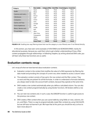
Introducing ISFILTERED, ISCROSSFILTERED
Two functions are very useful and might help you gain a better understanding of the propagation
of filter contexts. Moreover, learning them is a good way to introduce one of the most interesting
concepts of pivot table computation, that is, detection of the cell for which you are computing a value
from inside DAX.
These two functions aim to let you detect whether all the values of a column are visible in the
current filter context or not; they are:
■ ISFILTERED: returns TRUE or FALSE, depending on whether the column passed as an argument
has a direct filter on it, that is, it has been put on rows, columns, on a slicer or filter and the
filtering is happening for the current cell.
■ ISCROSSFILTERED returns TRUE or FALSE depending on whether the column has a filter be-
cause of automatic propagation of another filter and not because of a direct filter on it.
In this section, we are interested in using the functions to understand the propagation of filter
contexts. Thus, we are going to create dummy expressions, which are only useful as learning tools.
If you create a new measure with this definition:
[CategoryFilter] := ISFILTERED ( 'Product Category'[Category] )
This simple measure returns the value of the ISFILTERED function applied to the product category
name. You can then create a second measure that makes the same test with the product color. So the
code will be:
[ColorFilter] := ISFILTERED ( Product[ColorName] )
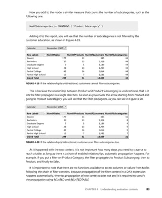
If you add both measures to a pivot table, placing the categories in a slicer and the colors on the
rows, the result will be similar to Figure 4-21.
The interesting part is that the category is never filtered because, even if we added a slicer, we did
not make a selection on it. The color, on the other hand, is always filtered on rows, because each row
has a specific color, but not in the grand total, because the filter context there does not include any
selection of products.
Note This behavior of the grand total, that is, no filter is applied from the ones coming
from rows and columns, is very useful whenever you want to modify the behavior of a
formula so that, at the grand total level, it shows a different value. In fact, you will check
ISFILTERED for an attribute present in the pivot table report in order to understand
whether the cell you are evaluating is in the inner part of the pivot table or if it is at the
grand total level.
[CategoryFilter] := ISFILTERED ( 'Product Category'[Category] )
[ColorFilter] := ISFILTERED ( Product[ColorName] )](https://image.slidesharecdn.com/librodaxbi-240516004012-1966db37/85/Formulas-dax-para-power-bI-de-microsoft-pdf-52-320.jpg)
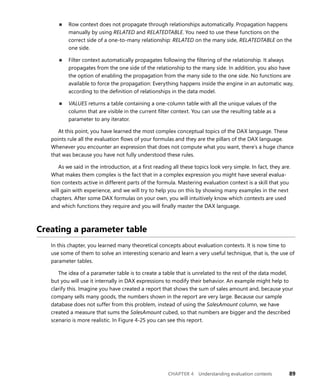
![CHAPTER 4 Understanding evaluation contexts 87
the product brand, you will get as a result only the brands of products of that specific color. When a
column is filtered because of a filter on another column, we say that the column is cross-filtered and
the ISCROSSFILTERED function detects this scenario.
If you add these two new measures to the data model that check, this time, the ISCROSSFILTERED
of color and category:
[CrossCategory] := ISCROSSFILTERED ( 'Product Category'[Category] )
[CrossColor] := ISCROSSFILTERED ( Product[Color] )
Then you will see the result shown in Figure 4-23.
FIGURE 4-23 Cross-filtering is visible using the ISCROSSFILTERED function.
You can see that color is cross-filtered and category is not. An interesting question, at this point,
is “Why is the category not filtered?” When you filter a color, you might expect to see only the
categories of product of that specific color. To answer the question you need to remember that the
category is not a column of the Product table. Instead, it is part of Product Category and the arrows
on the relationship do not let the relationship propagate. If you change the data model, enabling
bidirectional filtering on the full chain of relationships from Product to Product Category, then the
result will be different, as is visible in Figure 4-24.
[CrossCategory] := ISCROSSFILTERED ( 'Product Category'[Category] )
[CrossColor] := ISCROSSFILTERED ( Product[Color] )](https://image.slidesharecdn.com/librodaxbi-240516004012-1966db37/85/Formulas-dax-para-power-bI-de-microsoft-pdf-54-320.jpg)
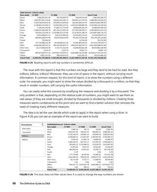
![CHAPTER 4 Understanding evaluation contexts 91
The interesting idea of the report is that you do not use the ShowValueAs slicer to filter data.
Instead, you will use it to change the scale used by the numbers. When the user selects Real Value,
the actual numbers will be shown. If Thousands is selected, then the actual numbers are divided by
one thousand and are shown in the same measure without having to change the layout of the pivot
table. The same applies to Millions and Billions.
To create this report, the first thing that you need is a table containing the values you want to
show on the slicer. In our example, made with Excel, we use an Excel table to store the scales. In a
more professional solution, it would be better to store the table in an SQL database. In Figure 4-27
you can see the content of such a table.
FIGURE 4-27 This Excel table will be the source for the slicer in the report.
Obviously, you cannot create any relationship with this table, because Sales does not contain any
column that you can use to relate to this table. Nevertheless, once the table is in the data model, you
can use the ShowValueAs column as the source for a slicer. Yes, you end up with a slicer that does
nothing, but some DAX code will perform the magic of reading user selections and further modifying
the content of the repor.
The DAX expression that you need to use for the measure is the following:
[ScaledSalesAmount] :=
IF (
HASONEVALUE ( Scale[DivideBy] ),
DIVIDE ( [Sales Amount], VALUES ( Scale[DivideBy] ) ),
[Sales Amount]
)
There are two interesting things to note in this formula:
■ The condition tested by the IF function is: HASONEVALUE ( Scale[ShowValueAs] ). This pattern
is very common: you check whether the column of the Scale table has only one value visible.
If the user did not select anything in the slicer, then all of the values of the column are visible
in the current filter context; that is, HASONEVALUE will return FALSE (because the column has
many different values). If, on the other hand, the user selected a single value, then only that
one is visible and HASONEVALUE will return TRUE. Thus, the condition reads as: “if the user has
selected a single value for ShowValueAs attribute.”
[ScaledSalesAmount] :=
IF (
HASONEVALUE ( Scale[DivideBy] ),
DIVIDE ( [Sales Amount], VALUES ( Scale[DivideBy] ) ),
[Sales Amount]
)](https://image.slidesharecdn.com/librodaxbi-240516004012-1966db37/85/Formulas-dax-para-power-bI-de-microsoft-pdf-58-320.jpg)
![92 The Definitive Guide to DAX
■ If a single value is selected, then you know that a single row is visible. Thus, you can compute
VALUES ( Scale[DivideBy] ) and you are sure that the resulting table contains only one column
and one row (the one visible in the filter context). DAX will convert the one-row-one-column
table returned by VALUES in a scalar value. If you try to use VALUES to read a single value
when the result is a table with multiple rows, you will get an error. However, in this specific
scenario, you are sure that the value returned will be only one, because of the previous
condition tested by the IF function.
Therefore, you can read the expression as: “If the user has selected a single value in the slicer, then
show the sales amount divided by the corresponding denominator, otherwise show the original sales
amount.” The result is a report that changes the values shown interactively, using the slicer as if it was
a button. Clearly, because the report uses only standard DAX formulas, it will work when deployed to
SharePoint or Power BI, too.
Parameter tables are very useful in building reports. We have shown a very simple (yet very
common) example, but the only limit is your imagination. You can create parameter tables to modify
the way a number is computed, to change parameters for a specific algorithm, or to perform other
complex operations that change the value returned by your DAX code.](https://image.slidesharecdn.com/librodaxbi-240516004012-1966db37/85/Formulas-dax-para-power-bI-de-microsoft-pdf-59-320.jpg)

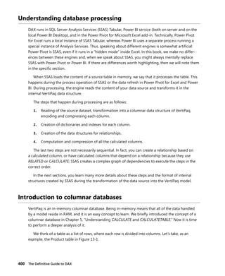
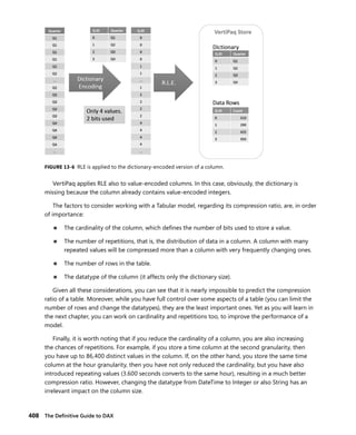
![CHAPTER 13 The VertiPaq engine 411
Hierarchies are of two types: attribute hierarchies and user hierarchies. They are data structures
used to improve performance of MDX queries. Because DAX does not have the concept of hierarchy
in the language, hierarchies are not interesting for the topics of this book.
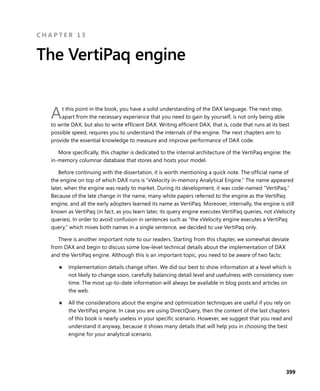
Relationships, on the other hand, play an important role in the VertiPaq engine and, for some
extreme optimizations, it is important to understand how they work. Later in this chapter, we will
cover the role of relationships in a query. Here we are only interested in defining what relationships
are, in terms of VertiPaq.
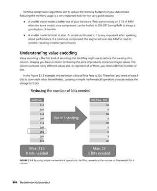
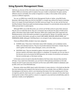
A relationship is a data structure that maps IDs in one table to row numbers in another table. For
example, consider the columns ProductKey in Sales and ProductKey in Products, used to build a relation-
ship between the two tables. Product[ProductKey] is a primary key. You know that it used value encoding
and no compression at all, because RLE could not reduce the size of a column without duplicated values.
On the other end, Sales[ProductKey] is likely dictionary encoded and compressed, because it probably
contains many repetitions. The data structures of the two columns are completely different.
Moreover, because you created the relationship, VertiPaq knows that you are likely to use it very
often, placing a filter on Product and expecting to filter Sales, too. If every time it needs to move a
filter from Product to Sales, VertiPaq had to retrieve values of Product[ProductKey], search them in the
dictionary of Sales[ProductKey], and finally retrieve the IDs of Sales[ProductKey] to place the filter, then
it would result in slow queries.
To improve query performance, VertiPaq stores relationships as pairs of IDs and row numbers.
Given the ID of a Sales[ProductKey], it can immediately find the corresponding rows of Product that
match the relationship. Relationships are stored in memory, as any other data structure of VertiPaq. In
Figure 13-7 you can see how the relationship between Sales and Product is stored.
FIGURE 13-7 The figure shows the relationship between Sales and Product.](https://image.slidesharecdn.com/librodaxbi-240516004012-1966db37/85/Formulas-dax-para-power-bI-de-microsoft-pdf-73-320.jpg)
![CHAPTER 13 The VertiPaq engine 417
Understanding materialization
Now that you have a basic understanding of how VertiPaq stores data in memory, you need to
learn what materialization is. Materialization is a step in query resolution that happens when using
columnar databases. Understanding when and how it happens is of paramount importance.
In order to understand what materialization is, look at this simple query:
EVALUATE
ROW (
"Result", COUNTROWS ( SUMMARIZE ( Sales, Sales[ProductKey] ) )
)
The result is the distinct count of product keys in the Sales table. Even if we have not yet covered
the query engine (we will, in Chapter 15, “Analyzing DAX query plans” and Chapter 16, “Optimizing
DAX”), you can already imagine how VertiPaq can execute this query. Because the only column
queried is ProductKey, it can scan that column only, finding all the values in the compressed structure
of the column. While scanning, it keeps track of values found in a bitmap index and, at the end, it
only has to count the bits that are set. Thanks to parallelism at the segment level, this query can run
extremely fast on very large tables and the only memory it has to allocate is the bitmap index to
count the keys.
The previous query runs on the compressed version of the column. In other words, there is no
need to decompress the columns and to rebuild the original table to resolve it. This optimizes the
memory usage at query time and reduces the memory reads.
The same scenario happens for more complex queries, too. Look at the following one:
EVALUATE
ROW (
"Result", CALCULATE (
COUNTROWS ( Sales ),
Product[Brand] = "Contoso"
)
)
This time, we are using two different tables: Sales and Product. Solving this query requires a bit
more effort. In fact, because the filter is on Product and the table to aggregate is Sales, you cannot
scan a single column.
If you are not yet used to columnar databases, you probably think that, to solve the query, you
have to iterate the Sales table, follow the relationship with Products, and sum 1 if the product brand is
Contoso, 0 otherwise. Thus, you might think of an algorithm similar to this one:
EVALUATE
ROW (
"Result", COUNTROWS ( SUMMARIZE ( Sales, Sales[ProductKey] ) )
)
EVALUATE
ROW (
"Result", CALCULATE (
COUNTROWS ( Sales ),
Product[Brand] = "Contoso"
)
)](https://image.slidesharecdn.com/librodaxbi-240516004012-1966db37/85/Formulas-dax-para-power-bI-de-microsoft-pdf-79-320.jpg)
![418 The Definitive Guide to DAX
EVALUATE
ROW (
"Result", SUMX (
Sales,
IF ( RELATED ( Product[Brand] ) = "Contoso", 1, 0 )
)
)
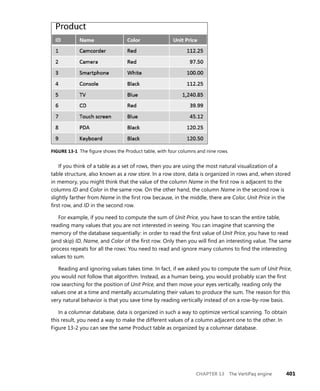
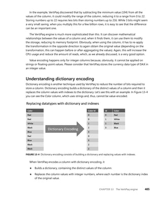
This is a simple algorithm, but it hides much more complexity than expected. In fact, if you
carefully think of the columnar nature of VertiPaq, this query involves three different columns:
■ Product[Brand] used to filter the Product table.
■ Product[ProductKey] used to follow the relationship between Product and Sales.
■ Sales[ProductKey] used on the Sales side to follow the relationship.
Iterating over Sales[ProductKey], searching the row number in Products scanning
Product[ProductKey], and finally gathering the brand in Product[Brand] would be extremely expensive
and require a lot of random reads to memory, negatively affecting performance. In fact, VertiPaq uses
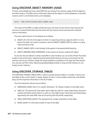
a completely different algorithm, optimized for columnar databases.
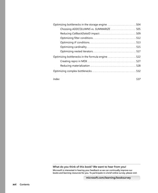
First, it scans Product[Brand] and retrieves the row numbers where Product[Brand] is Contoso. As
you can see in Figure 13-8, it scans the Brand dictionary (1), retrieves the encoding of Contoso, and
finally scans the segments (2) searching for the row numbers where ID equals to 0, returning the
indexes to the rows found (3).
FIGURE 13-8 The output of a brand scan is the list of rows where Brand equals Contoso.
EVALUATE
ROW (
"Result", SUMX (
Sales,
IF ( RELATED ( Product[Brand] ) = "Contoso", 1, 0 )
)
)](https://image.slidesharecdn.com/librodaxbi-240516004012-1966db37/85/Formulas-dax-para-power-bI-de-microsoft-pdf-80-320.jpg)
![CHAPTER 13 The VertiPaq engine 419
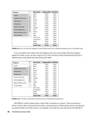
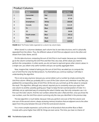
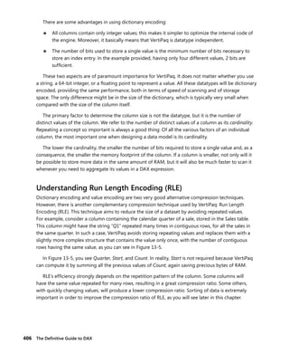
At this point, VertiPaq knows which rows in the Product table have the given brand. The relation-
ship between Product and Sales is based on Products[ProductKey] and, at this point VertiPaq knows
only the row numbers. Moreover, it is important to remember that the filter will be placed on Sales,
not on Products. Thus, in reality, VertiPaq does not need the values of Products[ProductKey], what it
really needs is the set of values of Sales[ProductKey], that is, the data IDs in the Sales table, not the
ones in Product.
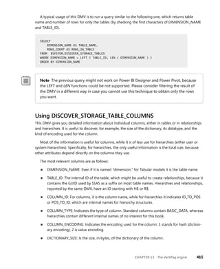
You might remember, at this point, that VertiPaq stores relationships as pairs of row numbers in
Product and data IDs in Sales[ProductKey]. It turns out that this is the perfect data structure to move
the filter from row numbers in Products to ProductKeys in Sales. In fact, VertiPaq performs a lookup
of the selected row numbers to determine the values of Sales[ProductKey] valid for those rows, as you
can see in Figure 13-9.
FIGURE 13-9 VertiPaq scans the product key to retrieve the IDs where brand equals Contoso.
The last step is to apply the filter on the Sales table. Since we already have the list of values of
Sales[ProductKey], it is enough to scan the Sales[ProductKey] column to transform this list of values
into row numbers and finally count them. If, instead of computing a COUNTROWS, VertiPaq had to
perform the SUM of a column, then it would perform another step transforming row numbers into
column values to perform the last step.
As you can see, this process is made up of simple table scanning where, at each step, you access a
single column. However, because data in a column is in the same memory area, VertiPaq sequentially
reads blocks of memory and performs simple operations on it, producing every time as output a
small data structure that is used in the following step.
The process of resolving a query in VertiPaq is very different from what common sense would
suggest. At the beginning, it is very hard to think in terms of columns instead of tables. The
algorithms of VertiPaq are optimized for column scanning; the concept of a table is a second-class
citizen in a columnar database.](https://image.slidesharecdn.com/librodaxbi-240516004012-1966db37/85/Formulas-dax-para-power-bI-de-microsoft-pdf-81-320.jpg)
![420 The Definitive Guide to DAX
Yet there are scenarios where the engine cannot use these algorithms and reverts to table
scanning. Look, for example, at the following query:
EVALUATE
ROW (
"Result", COUNTROWS (
SUMMARIZE ( Sales, Sales[ProductKey], Sales[CustomerKey] )
)
)
This query looks very innocent, and in its simplicity it shows the limits of columnar databases
(but also a row-oriented database faces the same challenge presented here). The query returns the
count of unique pairs of product and customer. This query cannot be solved by scanning separately
ProductKey and CustomerKey. The only option here is to build a table containing the unique pairs of
ProductKey and CustomerKey, and finally count the rows in it. Putting it differently, this time VertiPaq
has to build a table, even if with only a pair of columns, and it cannot execute the query directly on
the original store.
This step, that is, building a table with partial results, which is scanned later to compute the final
value, is known as materialization. Materialization happens for nearly every query and, by itself, it is
neither good nor bad. It all depends on the size of the table materialized. In fact, temporary tables
generated by materialization are not compressed (compressing them would take a lot of time, and
materialization happens at query time, when latency is extremely important).
It is significant to note that materialization does not happen when you access multiple columns
from a table. It all depends on what you have to do with those columns. For example, a query such as
the following does not need any materialization, even if it accesses two different columns:
EVALUATE
ROW (
"Result", SUMX (
Sales, Sales[Quantity] * Sales[Net Price]
)
)
VertiPaq computes the sum performing the multiplication while scanning the two columns, so
there is no need to materialize a table with Quantity and Net Price. Nevertheless, if the expression
becomes much more complex, or if you need the table for further processing (as it was the case in the
previous example, which required a COUNTROWS), then materialization might be required.
In extreme scenarios, materialization might use huge amounts of RAM (sometimes more than the
whole database) and generate very slow queries. When this happens, your only chance is to rewrite
the calculation or modify the model in such a way that VertiPaq does not need to materialize tables
to answer your queries. You will see some examples of these techniques in the following chapters of
this book.
EVALUATE
ROW (
"Result", COUNTROWS (
SUMMARIZE ( Sales, Sales[ProductKey], Sales[CustomerKey] )
)
)
EVALUATE
ROW (
"Result", SUMX (
Sales, Sales[Quantity] * Sales[Net Price]
)
)](https://image.slidesharecdn.com/librodaxbi-240516004012-1966db37/85/Formulas-dax-para-power-bI-de-microsoft-pdf-82-320.jpg)

![422 The Definitive Guide to DAX
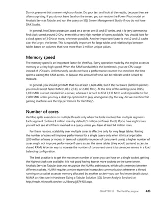
As you see, disk I/O performance is not in the list, because it is not important at all. There is a
condition (paging) where disk I/O affects performance, and we discuss it later in this section. However,
you should size the RAM of the system so that you will not have paging at all. Allocate your budget
on CPU and memory speed, memory size, and do not waste money on disk I/O bandwidth.
CPU model
The most important factors that affect the speed of code running in the VertiPaq are CPU clock
and model. Different CPU models might have a different performance at the same clock rate,
so considering the clock alone is not enough. The best practice is to run your own benchmark,
measuring the different performance in queries that stress the formula engine. An example of such a
query, on a model derived by Adventure Works, is the following:
EVALUATE
ROW (
"Test", COUNTROWS (
GENERATE (
TOPN (
8000,
CROSSJOIN (
ALL ( Reseller[ResellerKey] ),
ALL ( Reseller[GeographyKey] )
),
Reseller[ResellerKey]
),
ADDCOLUMNS (
SUMMARIZE (
Sales,
OrderDate[FullDate],
Products[ProductKey]
),
"Sales", CALCULATE ( SUM ( Sales[SalesAmount] ) )
)
)
)
)
You can download the sample workbook to test this query on your hardware here: http://www.sqlbi.
com/articles/choose-the-right-hardware-for-analysis-services-tabular/. Just open the Excel workbook
and run the previous query in DAX Studio, measuring the performance (more on this in Chapter 15).
You can try this query (which is intentionally slow and does not produce any meaningful result)
or similar ones. Using a query of a typical workload for your data model is certainly better, because
performance might vary on different hardware depending on the memory allocated to materialize
intermediate results (the query in the preceding code block has a minimal use of memory).
For example, this query runs in 8.1 seconds on an Intel i7-4770K 3.5 GHz, and in 12.4 seconds on
an Intel i7-2860QM 2.5 GHz. These CPUs run a desktop workstation and a notebook, respectively.
EVALUATE
ROW (
"Test", COUNTROWS (
GENERATE (
TOPN (
8000,
CROSSJOIN (
ALL ( Reseller[ResellerKey] ),
ALL ( Reseller[GeographyKey] )
),
Reseller[ResellerKey]
),
ADDCOLUMNS (
SUMMARIZE (
Sales,
OrderDate[FullDate],
Products[ProductKey]
),
"Sales", CALCULATE ( SUM ( Sales[SalesAmount] ) )
)
)
)
)](https://image.slidesharecdn.com/librodaxbi-240516004012-1966db37/85/Formulas-dax-para-power-bI-de-microsoft-pdf-84-320.jpg)
![541
DATESBETWEEN
D
data models
calculated columns and performance, 447–450
column cardinality and performance, 442–447
column storage, choosing columns for, 451–453
column storage, optimization of, 453–455
denormalization, 434–442
gathering information about model, 425–434
cost of a column hierarchy, 430–434
dictionary size for each column, 428–429
number of rows in a table, 426–427
number of unique values per column, 427–429
total cost of table, 433–434
overview of, 1–3
relationship directions, 3–4
VertiPaq Analyzer, performance optimization and, 510
data types
aggregate functions, numeric and non-numeric
values, 35–37
DAX syntax, overview of, 18–21
information functions, overview, 39
database processing
columnar databases, introduction to, 400–403
Dynamic Management Views, use of, 413–416
materialization, 417–420
segmentation and partitioning, 412
VertiPaq compression, 403–411
best sort order, finding of, 409–410
dictionary encoding, 405–406
hierarchies and relationships, 410–411
re-encoding, 409
Run Length Encoding (RLE), 406–408
value encoding, 404–405
VertiPaq, hardware selection, 421–424
VertiPaq, understanding of, 400
datacaches. See also formulas, optimization of
CallbackDataID, use of, 483–488
DAX Studio, event tracing with, 467–470
formula engine (FE), overview, 458
parallelism and datacache, understanding of, 480–481
query plans, reading of, 488–494
server timings and query plans, analysis of, 500–503
storage engine (VertiPaq), overview, 459
VertiPaq cache and, 481–483
VertiPaq SE query cache match, 464
date. See also Date table
column cardinality and performance, 443–447
date and time functions, overview, 42
sales per day calculations, 143–150
time intelligence, introduction to, 155
working days, computing differences in, 150–151
DATE
conversion functions, overview, 41–42
date and time functions, overview, 42
date table names, 157
Date (DateTime), syntax, 18, 20
Date table
aggregating and comparing over time, 168
computing differences over previous periods,
174–175
computing periods from prior periods,
171–174
year-, quarter-, and month-to-date, 168–171
CALENDAR and CALENDARAUTO, use of, 157–160
closing balance over time, 178–188
CLOSINGBALANCE, 184–188
custom calendars, 200–201
custom comparisons between periods,
210–211
noncontiguous periods, computing over,
206–209
weeks, working with, 201–204
year-, quarter-, and month-to-date, 204–205
DATEADD, use of, 191–196
drillthrough operations, 200
FIRSTDATE and LASTDATE, 196–199
FIRSTNOBLANK and LASTNOBLANK, 199–200
Mark as Date Table, use of, 166–168
moving annual total calculations, 175–178
multiple dates, working with, 160–164
naming of, 157
OPENINGBALANCE, 184–188
periods to date, understanding, 189–191
time intelligence, advanced functions, 188
time intelligence, introduction to, 155, 164–166
Date, cumulative total calculations, 134–136
DATEADD
previous year, month, quarter comparisons,
171–174
use of, 191–196
Date[DateKey], Mark as Date Table, 166–168
DateKey, cumulative total calculations, 134–136
DATESBETWEEN
moving annual total calculations, 175–178
working days, computing differences, 151](https://image.slidesharecdn.com/librodaxbi-240516004012-1966db37/85/Formulas-dax-para-power-bI-de-microsoft-pdf-91-320.jpg)