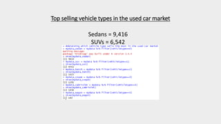
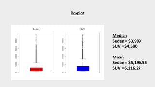
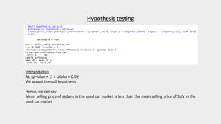
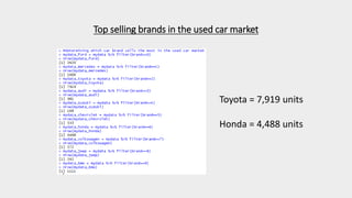
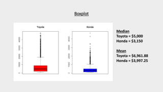
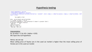
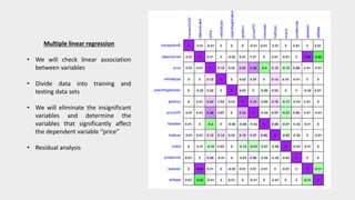
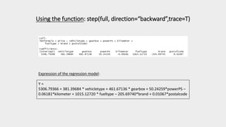
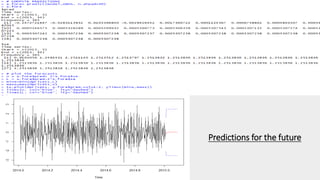
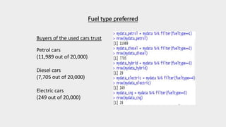
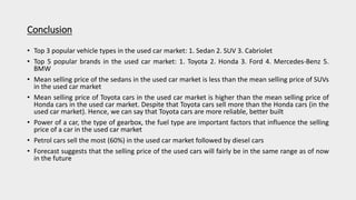
The document analyzes used car e-commerce statistics. It finds that sedans and SUVs are the most popular vehicle types sold used, while Toyota and Honda are the most popular brands. The mean sale price of sedans is lower than SUVs, and the mean price of Toyotas is higher than Hondas. A multiple linear regression model shows factors like vehicle power, gearbox type, and fuel type significantly impact sale price. Finally, it forecasts that future used car prices will remain stable.

1. “Used Car E-Commerce Stats
for Buyers, Sellers & Advertisers”
Prepared by,
Rohit G. Vaze
rvaze@hawk.iit.edu
Group number: 175

2. Introduction
• High increase in used (2nd hand) car sales in recent years
• Used cars: Fairly good condition, low cost
• E-commerce websites have triggered used car sales
• Popular E-commerce website for selling used cars: eBay
• Which are the popular brands in the used car market?
• Which are the popular vehicle types in the used car market?
• The selling price (ad price) of a used car depends on what factors?
• How will the used car prices be in the future?

3. Data set
Used car data set (header and 20,000 rows)

4. Checking for the missing values
No missing values

5. Top selling vehicle types in the used car market
Sedans = 9,416
SUVs = 6,542

6. Boxplot
Median
Sedan = $3,999
SUV = $4,500
Mean
Sedan = $5,196.55
SUV = 6,116.27

7. Hypothesis testing
Interpretation
As, (p-value = 1) > (alpha = 0.05)
We accept the null hypothesis
Hence, we can say
Mean selling price of sedans in the used car market is less than the mean selling price of SUV in the
used car market

8. Top selling brands in the used car market
Toyota = 7,919 units
Honda = 4,488 units

9. Boxplot
Median
Toyota = $5,000
Honda = $3,150
Mean
Toyota = $6,961.88
Honda = $3,997.25

10. Hypothesis testing
Interpretation
As, (p-value < 2.2e-16) < (alpha = 0.05)
We reject the null hypothesis
Hence, we can say
Mean selling price of Toyota cars in the used car market is higher than the mean selling price of
Honda cars in the used car market

11. Multiple linear regression
• We will check linear association
between variables
• Divide data into training and
testing data sets
• We will eliminate the insignificant
variables and determine the
variables that significantly affect
the dependent variable “price”
• Residual analysis

12. Correlation plot

13. Values of the correlations
High correlation
powerPS, price = 0.4812459
gearbox, price = 0.2236955
vehicletype, price = 0.119897
fueltype, price = 0.1153594

14. Eliminating the insignificant independent variables

15. Significant independent variables
Significant independent variables
• vehicletype
• gearbox
• powerPS
• kilometer
• fueltype
• brand
• postalcode

16. Using the function: step(full, direction=“backward”,trace=T)
Expression of the regression model:
Y =
5306.79366 + 381.39684 * vehicletype + 461.67136 * gearbox + 50.24259*powerPS –
0.06181*kilometer + 1015.12720 * fueltype – 205.69740*brand + 0.01067*postalcode

17. VIF values
vehicletype =
1.028207
gearbox = 1.166104
powerPS = 1.190127
kilometer = 1.019822
fueltype = 1.060202
brand = 1.081085
postalcode = 1.008306
VIF < 5,
No collinearity
problem

18. Checking the normality of the given data
Predicted vs Residual Plot
Since, majority data points
are concentrated around
the regression line, we can
say that the data is
normally distributed
Predicted vs Residual Plot
As majority data points lie
on the regression line we
can say that the data is
normally distributed

19. Residual analysis and predictions
Choosing the best model
with least RMSE value

20. ANOVA (for the independent variable ‘vehicletype’)
Null hypothesis:
Group means price of all cars with different vehicletypes are equal
Alternative hypothesis:
Group means price of all cars with different vehicletypes are not
equal
Interpretation:
(p-value < 2e-16) < (alpha = 0.05)
Hence, we reject null hypothesis
Hence, we can say that group means of all cars with different
vehicletypes are not equal

21. ANOVA (for the independent variable ‘brand’)
Null hypothesis:
Group means price of all cars with different brands are equal
Alternative hypothesis:
Group means price of all cars with different brands are not equal
Interpretation:
(p-value < 2e-16) < (alpha = 0.05)
Hence, we reject null hypothesis
Hence, we can say that group means of all cars with different brands
are not equal

22. ANOVA (for the independent variable ‘fueltype’)
Null hypothesis:
Group means price of all cars with different fueltypes are equal
Alternative hypothesis:
Group means price of all cars with different fueltypes are not equal
Interpretation:
(p-value < 2e-16) < (alpha = 0.05)
Hence, we reject null hypothesis
Hence, we can say that group means of all cars with different
fueltypes are not equal

23. Time series analysis and forecasting
• Loading the data set and required libraries
• Normality test: Histogram, QQ plot, Jarque-Bera test
• Ljung box test, ACF plots, PACF plots
• Differencing
• Build different models AR, MA, ARMA, ARIMA
• Future predictions

24. Jarque-bera test and histogram and QQ plot before differencing
As,
(p-value < 2.2e-16) < (alpha = 0.05),
we can state that the distribution is
normal

25. Time series plots
Mean and variance look constant with time: Stationary series

26. Normality test on differenced time series object
Majority points lie on the line. Hence, we can say
that the distribution is normal

27. Checking for serial correlation
Null hypothesis:
Series is not correlated and autocorrelations of time series object is
zero
Alternative hypothesis:
Series is correlated
As,
p-value < (alpha = 0.05)
We reject the null hypothesis
Hence,
We can say that serial correlation exists

28. Selecting the best model based on AIC value
Model using EACF:
AIC = 981.97

29. Selecting the best model based on AIC value
Model using AR:
AIC = 1124.99
Model using MA:
AIC = 979.32
Model MA is the best model as the AIC value is the lowest in its case

30. Plots

31. Residual analysis for MA model

32. Residual analysis for MA model
Ljung-box test result states that the residuals is independent
(close to white noise series)
Our model is adequate

33. Predictions for the future

34. Fuel type preferred
Buyers of the used cars trust
Petrol cars
(11,989 out of 20,000)
Diesel cars
(7,705 out of 20,000)
Electric cars
(249 out of 20,000)

35. Conclusion
• Top 3 popular vehicle types in the used car market: 1. Sedan 2. SUV 3. Cabriolet
• Top 5 popular brands in the used car market: 1. Toyota 2. Honda 3. Ford 4. Mercedes-Benz 5.
BMW
• Mean selling price of the sedans in the used car market is less than the mean selling price of SUVs
in the used car market
• Mean selling price of Toyota cars in the used car market is higher than the mean selling price of
Honda cars in the used car market. Despite that Toyota cars sell more than the Honda cars (in the
used car market). Hence, we can say that Toyota cars are more reliable, better built
• Power of a car, the type of gearbox, the fuel type are important factors that influence the selling
price of a car in the used car market
• Petrol cars sell the most (60%) in the used car market followed by diesel cars
• Forecast suggests that the selling price of the used cars will fairly be in the same range as of now
in the future

36. THANK YOU