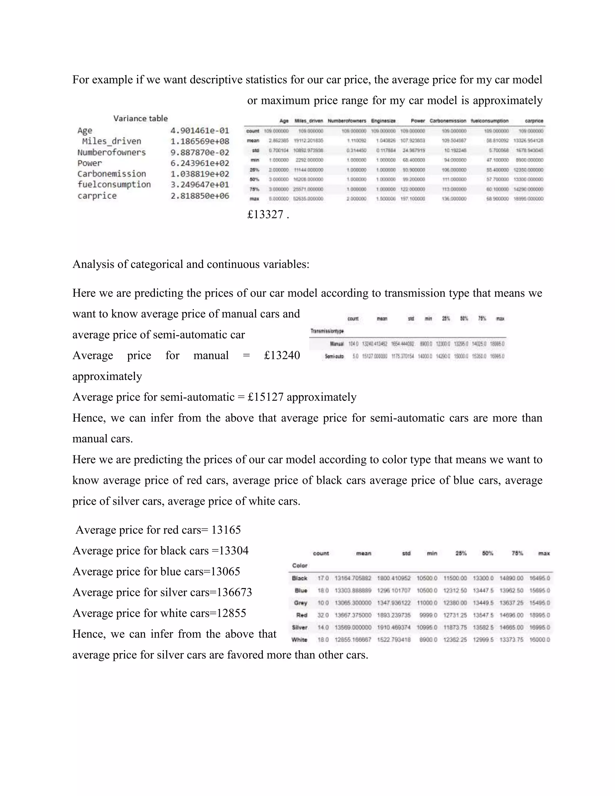
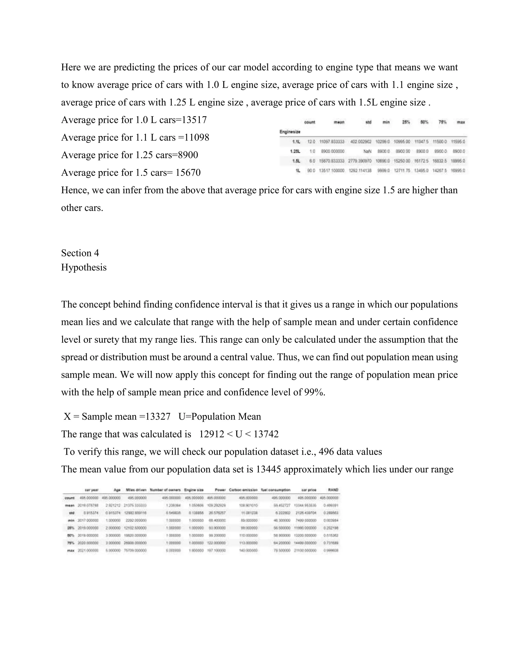
SlideShare a Scribd company logo
1 of 13
Coursework Details: 2nd Hand Car Market Case Study
EXECUTIVE SUMMARY
This report analyzes secondhand Ford Fiesta in B74JP and recommends the changes in prices due
to change in car age, mileage, and engine power.
The used market is a sizable space, making the process of purchasing or selling a car intimidating.
We have examined the variables that affect our car's price and the effect they have on the auto
industry. Age, mileage, and engine power of our car are determining factors in price. To compare
the averages of each of these variables and determine the links between them, we examined the
central tendency and dispersion of prices as well as these other characteristics. We identify their
intra and inter relationships as well as the effects of these interactions on the predictor after
performing various statistical tests.
We also recognize the significance of the size and strength of these linkages. We did specific
analyses to develop a model to determine whether the strength of the connection affects the overall
relationship
TABLE OF CONTENT
Executive Summary……………………………………………………………………………
Contents
Section 1 .......................................................................................................................................................4
Introduction...............................................................................................................................................4
Section 2 .......................................................................................................................................................5
Visualizations............................................................................................................................................5
Section 3 .......................................................................................................................................................6
Descriptive statistics .................................................................................................................................6
Section 4 .......................................................................................................................................................8
Hypothesis ................................................................................................................................................8
Section 5 .......................................................................................................................................................9
Correlation Analysis .................................................................................................................................9
Section 6 .....................................................................................................................................................11
Regression analysis.................................................................................................................................11
Section 7 .....................................................................................................................................................13
Conclusion ..............................................................................................................................................13
Section 8 .....................................................................................................................................................13
References...............................................................................................................................................13
Section 1
Introduction
We want to forecast the typical used car pricing for Ford fiesta in postal code B74JP gathered from
population. We summarize car data in an organized way by explaining the relationship between
different variables in a sample. To ascertain which elements, have the greatest influence on price
and which ones have no impact at all, we anticipate various correlations.
The Source of our data is https://heycar.co.uk/used-cars. After extracting relevant data from our
source to an excel file, the major limitation was of missing values and manipulation of those values
was crucial to accurately analyze data and interpret its output coherently. We are cleaning data
without changing the real context of the data by either adding or deleting values or removing
anomalies. In our dataset, we filter out blank or missing values to check the number of missing
values in our dataset. Then for this dataset we have deleted all the missing values as they were low
in number, and they were not making much of an impact on the meaning of the dataset. In this
dataset, we are adopting simple random sampling because it gives each person or member of a
group an equal and just chance of being chosen by randomly selecting a small portion of persons
or members from the total population. (“Random Sampling - Overview, Types, Importance,
Example”) Also, simple random sampling is required while finding the intervals in which the
average of the whole population lies. [2]https://corporatefinanceinstitute.com/resources/data-
science/random-sampling/
We are examining 5-year car data since it will not only provide us knowledge from that time period
about which cars are popular based on their performance but also help us to predict more
accurately. Consequently, it will be simpler for us to decide which to buy or sell.
Section 2
Visualizations
We can visualize from the above graph the
distribution of secondhand ford fiesta in B7 4JP
Most cars fall in the interval of prices £12000 to
£14000. Also, it can be observed that people
prefer to buy manual cars as compared to semi-
automatic cars. The manual cars fall under the car
price of £13000 range and semi-automatic fall
under £14000
The relationship between two Ford Fiesta
attributes and how their costs vary may be seen in
the graph above. We are considering engine size
and transmission type as our attributes.
Cars with engine size 1.0 L have both manual and
semi-automatic variants as compared to engine
size 1.5L, 1.25L and 1.1L which have only manual variants. Moreover, we see price of manual
and engine size 1.5 has the highest price point in our area.
The association between miles driven and
Ford Fiesta costs may be seen in the graph
above. Since there is some modest negative
linearity between these factors, the cost of
the car decreases with increased driving.
We have created visualizations with elements that are true representations of our data. The labels
in the graphs above clearly depict values, and margins of our graphs are starting from zero.
Moreover, in the bar graphs and histograms the bars on the graph follow symmetrical order. There
is similarity of colors and connection, and graphs also follow enclosure principle which means
every graph is having a border or a boundary.
Section 3
Descriptive statistics
After data extraction and cleaning of the sample, we divide the dataset into two parts or two set of
variables i.e., one part entails all the numeric values that have some mathematical connotation and
other part entails the values that are non-numeric. These numeric values are called Continuous
variables and non-numeric are called categorical variables.
Categorical Variables Continuous variables
Car Price Transmission type
Miles driven by the car Color of the car
Number of previous owners of the
car
Engine size
Engine Power
Carbon Emission
Fuel Consumption
Car year
Age (calculated from 2022- car year)
We can calculate descriptive statistics for the numeric data only.
The descriptive statistics incudes the average values in a dataset, the middle value of a dataset and
the number that occurs more frequently in a data set. Also, we get to know about the distance or
deviation of individual values from the average values and through that we are able to calculate a
standard that helps us to understand which values are fall under normal range and which are less
than normal and more than normal.
For example if we want descriptive statistics for our car price, the average price for my car model
or maximum price range for my car model is approximately
£13327 .
Analysis of categorical and continuous variables:
Here we are predicting the prices of our car model according to transmission type that means we
want to know average price of manual cars and
average price of semi-automatic car
Average price for manual = £13240
approximately
Average price for semi-automatic = £15127 approximately
Hence, we can infer from the above that average price for semi-automatic cars are more than
manual cars.
Here we are predicting the prices of our car model according to color type that means we want to
know average price of red cars, average price of black cars average price of blue cars, average
price of silver cars, average price of white cars.
Average price for red cars= 13165
Average price for black cars =13304
Average price for blue cars=13065
Average price for silver cars=136673
Average price for white cars=12855
Hence, we can infer from the above that
average price for silver cars are favored more than other cars.
Here we are predicting the prices of our car model according to engine type that means we want
to know average price of cars with 1.0 L engine size, average price of cars with 1.1 engine size ,
average price of cars with 1.25 L engine size , average price of cars with 1.5L engine size .
Average price for 1.0 L cars=13517
Average price for 1.1 L cars =11098
Average price for 1.25 cars=8900
Average price for 1.5 cars= 15670
Hence, we can infer from the above that average price for cars with engine size 1.5 are higher than
other cars.
Section 4
Hypothesis
The concept behind finding confidence interval is that it gives us a range in which our populations
mean lies and we calculate that range with the help of sample mean and under certain confidence
level or surety that my range lies. This range can only be calculated under the assumption that the
spread or distribution must be around a central value. Thus, we can find out population mean using
sample mean. We will now apply this concept for finding out the range of population mean price
with the help of sample mean price and confidence level of 99%.
X = Sample mean =13327 U=Population Mean
The range that was calculated is 12912 < U < 13742
To verify this range, we will check our population dataset i.e., 496 data values
The mean value from our population data set is 13445 approximately which lies under our range
There is a one claim that average car price of the sample of our dataset is like the average car price
of UK taken from motors.co.uk. In order, to check that this statement is right or wrong we use a
method called hypothesis testing. In hypothesis testing, we have two statements, one is called null
hypothesis other is called alternate hypothesis. For this claim our null hypothesis is that average
price=13773
And alternate hypothesis is average price is not equal to 13773. In order to prove this, claim we
use one-sample t-test. After carrying out this test we
were able to determine that the average price of the
sample is not in line with the average price taken
from a different source.
Here p value =0.0065 much less than 0.05 so we reject null hypothesis.
Source: https://www.motors.co.uk/
There is another claim if there is a relationship between two categorical values i.e., number of
owners and transmission type. In order, to check that this statement is right or wrong, we will do
hypothesis testing, here the null value would be that there exists relationship and alternate
hypothesis would be that no relationship exists.
We will do chi square test to find out if there is statistically significant relationship between number
of owners and transmission type. We will first
create a table that shows multi-variate relationship
between these two variables. The table is grouping categorical variables with respect to their
counts. The p value is 0.941163926818371 that is greater than 0.05 so we reject null hypothesis
that means there is no dependency between number of owners and transmission type.
Section 5
Correlation Analysis
The Pearson Correlation Coefficient (R ) evaluates the strength and direction of a link between
two variables. R's value is always between -1 and +1.
If R=0 it does not mean that there exists no relationship, it means that there is no linear relationship.
if R=1 we say it is positively corelated that means the independent variable is directly proportional
to dependent variable and if R= -1, it means the independent variable is indirectly proportional to
dependent variable.
https://towardsdatascience.com/the-importance-of-r-in-data-science-
6b394d48fa50#:~:text=and%20its%20use-,What%20is%20r%3F,1%20and%20a%20%2B1).
For our dataset, the dependent variable is car price and using correlation coefficient we will figure
out the strength of relationship of car price with other car characteristics. Also, for ranges -0.3<r<-
0.1 and 0.3<r<0.1, we say there is a small strength of association, similarly in case of -0.3<r<-0.5
we say there is a medium
strength of association and
same goes for the positive
counterpart and if r lies in
range -0.5<r<-1.0 and -
0.5<r<-1.0 there is large
strength of association.
From the matrix given we
see that car price has a
positive correlation with car
power that means the car
with more power will be
expensive as compared to car with less power. Moreover, r value for car prices and silver color
comes under small strength of association. We can conclude from our matrix that correlation does
not state how much the impact will be, it always conveys the strength of the relationship between
variables.
Section 6
Regression analysis
Parsimonious is nothing but set of rules is that utilizes no more "things" than are essential; in the
case of parsimonious models, those "things"
are parameters. Models with optimal
parsimony, or the precise number of predictors
required to fully describe the model, are called
parsimonious.
https://www.statisticshowto.com/parsimonious-model/
We check parsimony of our model through the principle of normality, which states that the values
of the data are normally distributed if they fall nearly along a straight line at a 45-degree angle.
From the above graph, we can infer that our model follows the assumption of normality and is
parsimonious in nature.
To check the adequacy for our model, we need to satisfy three different principles:
1. Principle of linearity: This principle
states that if it appears that the plotted
points might all lie along a straight line,
indicating that the two variables have linear
relationship.
2. Principle of Homoscedasticity: This
principles states if the plotted points on a
scatter graph are randomly scattered that
forms no shape.
3. Principle of independence of errors: This principle states that the residuals in positive
region and negative region are almost equal then there exists independence of errors.
From the scatter graph below, we see our model follows all three principles. Hence, it follows
principle of adequacy.
From the model summary table, we infer
that the adjusted r square is 0.693 and through the above graphs we concluded that our model is
parsimonious and adequate. The adjusted r square can be improved but there are certain
independent variables which have extremely high significance values, and they might not have
substantial impact on the car price. And to know which variables impact the car price the most and
least we carry out residual analysis which means removing independent variables with high
significance values given in the coefficient table. We can see from the Coefficient table given
above, es15 that means engine size of 1.5L has highest significance value that is 0.851 which
means that it has exceptionally negligible impact on the car price of our model, and it needs to be
removed. We will do this process repeatedly until we have variables with significance level closer
to 0.001 but not more than 0.05. This process is of removing and checking the adjusted r square is
called residual analysis. In the coefficient table, to know the magnitude of impact of our
independent variables on our car price we refer to the standardized coefficients beta column. After
analyzing the beta columns, we verify that engine size has the lowest impact on our car price so
we will remove this variable first.
We will conduct this process until the significance values in our coefficient table are closer to
0.001 but not more than 0.05.
After conducting residual analysis, we have produced
an r square value of 0.705 and the significance values for all our independent variables are closer
to 0.001 and less than 0.05.
Section 7
Conclusion
Thus, we can conclude that prices of semi-automatic ford fiesta with engine size of 1.1 liters can
be 70% predicted through car’s age, miles driven, power and fuel consumption.
This model is adequate and Parsimonious; hence we would recommend this model for buyers and
sellers so that they have a clear view about how car prices change according to different choices
of engine size, power, and age of car.
Section 8
References

More Related Content

Similar to Descriptive Analysis.docx

The last part of the analysis will examine the relationship between MPG and o...
The last part of the analysis will examine the relationship between MPG and o...The last part of the analysis will examine the relationship between MPG and o...
The last part of the analysis will examine the relationship between MPG and o...
wamorena lempadi
 
NPD Aftermarket Perspectives
NPD Aftermarket PerspectivesNPD Aftermarket Perspectives
NPD Aftermarket Perspectives
buddhand
 
Final Economic Proposal for RYNO Bike
Final Economic Proposal for RYNO BikeFinal Economic Proposal for RYNO Bike
Final Economic Proposal for RYNO Bike
Julie Bentley
 
Safer Drivers - An Analysis of Driver Characteristics in Car Fatalities
Safer Drivers - An Analysis of Driver Characteristics in Car FatalitiesSafer Drivers - An Analysis of Driver Characteristics in Car Fatalities
Safer Drivers - An Analysis of Driver Characteristics in Car Fatalities
Ryan Schuldt
 
BigData_HW3_Boris_Menshikov_15613416.pptx
BigData_HW3_Boris_Menshikov_15613416.pptxBigData_HW3_Boris_Menshikov_15613416.pptx
BigData_HW3_Boris_Menshikov_15613416.pptx
MorisMenshen
 
A Wish Called $quander
A Wish Called $quanderA Wish Called $quander
A Wish Called $quander
Catalystian
 
Line, bar and Pie graphsNameInstitution 1.docx
Line, bar and Pie graphsNameInstitution 1.docxLine, bar and Pie graphsNameInstitution 1.docx
Line, bar and Pie graphsNameInstitution 1.docx
smile790243
 
Cab_Aggregator_Services.pdf
Cab_Aggregator_Services.pdfCab_Aggregator_Services.pdf
Cab_Aggregator_Services.pdf
SouMYa549418
 

Similar to Descriptive Analysis.docx (20)

Household transportation cost management
Household transportation cost managementHousehold transportation cost management
Household transportation cost management
 
The last part of the analysis will examine the relationship between MPG and o...
The last part of the analysis will examine the relationship between MPG and o...The last part of the analysis will examine the relationship between MPG and o...
The last part of the analysis will examine the relationship between MPG and o...
 
Mercer Capital's Value Focus: Auto Dealer Industry | Year-End 2018
Mercer Capital's Value Focus: Auto Dealer Industry | Year-End 2018Mercer Capital's Value Focus: Auto Dealer Industry | Year-End 2018
Mercer Capital's Value Focus: Auto Dealer Industry | Year-End 2018
 
NPD Aftermarket Perspectives
NPD Aftermarket PerspectivesNPD Aftermarket Perspectives
NPD Aftermarket Perspectives
 
Total Cost of Ownership: A Gas vs. Diesel Comparison
Total Cost of Ownership: A Gas vs. Diesel ComparisonTotal Cost of Ownership: A Gas vs. Diesel Comparison
Total Cost of Ownership: A Gas vs. Diesel Comparison
 
Car Study &amp; Statistics
Car Study &amp; StatisticsCar Study &amp; Statistics
Car Study &amp; Statistics
 
Final Economic Proposal for RYNO Bike
Final Economic Proposal for RYNO BikeFinal Economic Proposal for RYNO Bike
Final Economic Proposal for RYNO Bike
 
Safer Drivers - An Analysis of Driver Characteristics in Car Fatalities
Safer Drivers - An Analysis of Driver Characteristics in Car FatalitiesSafer Drivers - An Analysis of Driver Characteristics in Car Fatalities
Safer Drivers - An Analysis of Driver Characteristics in Car Fatalities
 
BigData_HW3_Boris_Menshikov_15613416.pptx
BigData_HW3_Boris_Menshikov_15613416.pptxBigData_HW3_Boris_Menshikov_15613416.pptx
BigData_HW3_Boris_Menshikov_15613416.pptx
 
Prediction of Car Price using Linear Regression
Prediction of Car Price using Linear RegressionPrediction of Car Price using Linear Regression
Prediction of Car Price using Linear Regression
 
A Wish Called $quander
A Wish Called $quanderA Wish Called $quander
A Wish Called $quander
 
White Paper
White PaperWhite Paper
White Paper
 
Line, bar and Pie graphsNameInstitution 1.docx
Line, bar and Pie graphsNameInstitution 1.docxLine, bar and Pie graphsNameInstitution 1.docx
Line, bar and Pie graphsNameInstitution 1.docx
 
Scenaria Perspective #1 - 2025 CAFE Compliance Costs
Scenaria Perspective #1 - 2025 CAFE Compliance CostsScenaria Perspective #1 - 2025 CAFE Compliance Costs
Scenaria Perspective #1 - 2025 CAFE Compliance Costs
 
Cab_Aggregator_Services.pdf
Cab_Aggregator_Services.pdfCab_Aggregator_Services.pdf
Cab_Aggregator_Services.pdf
 
Carculate
Carculate Carculate
Carculate
 
Global Hybrid Cars - Sep'13
Global Hybrid Cars - Sep'13Global Hybrid Cars - Sep'13
Global Hybrid Cars - Sep'13
 
Hybrid car sales (Ford case )
Hybrid car sales (Ford case )Hybrid car sales (Ford case )
Hybrid car sales (Ford case )
 
Motor vehicle engine, power train and parts global market report 2018
Motor vehicle engine, power train and parts global market report 2018Motor vehicle engine, power train and parts global market report 2018
Motor vehicle engine, power train and parts global market report 2018
 
Current market conditionsca_week3
Current market conditionsca_week3Current market conditionsca_week3
Current market conditionsca_week3
 

Recently uploaded

Vip Mumbai Call Girls Marol Naka Call On 9920725232 With Body to body massage...
Vip Mumbai Call Girls Marol Naka Call On 9920725232 With Body to body massage...Vip Mumbai Call Girls Marol Naka Call On 9920725232 With Body to body massage...
Vip Mumbai Call Girls Marol Naka Call On 9920725232 With Body to body massage...
amitlee9823
 
Call Girls In Doddaballapur Road ☎ 7737669865 🥵 Book Your One night Stand
Call Girls In Doddaballapur Road ☎ 7737669865 🥵 Book Your One night StandCall Girls In Doddaballapur Road ☎ 7737669865 🥵 Book Your One night Stand
Call Girls In Doddaballapur Road ☎ 7737669865 🥵 Book Your One night Stand
amitlee9823
 
Call Girls Bannerghatta Road Just Call 👗 7737669865 👗 Top Class Call Girl Ser...
Call Girls Bannerghatta Road Just Call 👗 7737669865 👗 Top Class Call Girl Ser...Call Girls Bannerghatta Road Just Call 👗 7737669865 👗 Top Class Call Girl Ser...
Call Girls Bannerghatta Road Just Call 👗 7737669865 👗 Top Class Call Girl Ser...
amitlee9823
 
Al Barsha Escorts $#$ O565212860 $#$ Escort Service In Al Barsha
Al Barsha Escorts $#$ O565212860 $#$ Escort Service In Al BarshaAl Barsha Escorts $#$ O565212860 $#$ Escort Service In Al Barsha
Al Barsha Escorts $#$ O565212860 $#$ Escort Service In Al Barsha
AroojKhan71
 
FESE Capital Markets Fact Sheet 2024 Q1.pdf
FESE Capital Markets Fact Sheet 2024 Q1.pdfFESE Capital Markets Fact Sheet 2024 Q1.pdf
FESE Capital Markets Fact Sheet 2024 Q1.pdf
MarinCaroMartnezBerg
 
Call Girls Hsr Layout Just Call 👗 7737669865 👗 Top Class Call Girl Service Ba...
Call Girls Hsr Layout Just Call 👗 7737669865 👗 Top Class Call Girl Service Ba...Call Girls Hsr Layout Just Call 👗 7737669865 👗 Top Class Call Girl Service Ba...
Call Girls Hsr Layout Just Call 👗 7737669865 👗 Top Class Call Girl Service Ba...
amitlee9823
 
Call Girls Indiranagar Just Call 👗 9155563397 👗 Top Class Call Girl Service B...
Call Girls Indiranagar Just Call 👗 9155563397 👗 Top Class Call Girl Service B...Call Girls Indiranagar Just Call 👗 9155563397 👗 Top Class Call Girl Service B...
Call Girls Indiranagar Just Call 👗 9155563397 👗 Top Class Call Girl Service B...
only4webmaster01
 
CHEAP Call Girls in Saket (-DELHI )🔝 9953056974🔝(=)/CALL GIRLS SERVICE
CHEAP Call Girls in Saket (-DELHI )🔝 9953056974🔝(=)/CALL GIRLS SERVICECHEAP Call Girls in Saket (-DELHI )🔝 9953056974🔝(=)/CALL GIRLS SERVICE
CHEAP Call Girls in Saket (-DELHI )🔝 9953056974🔝(=)/CALL GIRLS SERVICE
9953056974 Low Rate Call Girls In Saket, Delhi NCR
 

Recently uploaded (20)

Halmar dropshipping via API with DroFx
Halmar  dropshipping  via API with DroFxHalmar  dropshipping  via API with DroFx
Halmar dropshipping via API with DroFx
 
Vip Mumbai Call Girls Marol Naka Call On 9920725232 With Body to body massage...
Vip Mumbai Call Girls Marol Naka Call On 9920725232 With Body to body massage...Vip Mumbai Call Girls Marol Naka Call On 9920725232 With Body to body massage...
Vip Mumbai Call Girls Marol Naka Call On 9920725232 With Body to body massage...
 
Call Girls In Doddaballapur Road ☎ 7737669865 🥵 Book Your One night Stand
Call Girls In Doddaballapur Road ☎ 7737669865 🥵 Book Your One night StandCall Girls In Doddaballapur Road ☎ 7737669865 🥵 Book Your One night Stand
Call Girls In Doddaballapur Road ☎ 7737669865 🥵 Book Your One night Stand
 
VIP Model Call Girls Hinjewadi ( Pune ) Call ON 8005736733 Starting From 5K t...
VIP Model Call Girls Hinjewadi ( Pune ) Call ON 8005736733 Starting From 5K t...VIP Model Call Girls Hinjewadi ( Pune ) Call ON 8005736733 Starting From 5K t...
VIP Model Call Girls Hinjewadi ( Pune ) Call ON 8005736733 Starting From 5K t...
 
Call Girls Bannerghatta Road Just Call 👗 7737669865 👗 Top Class Call Girl Ser...
Call Girls Bannerghatta Road Just Call 👗 7737669865 👗 Top Class Call Girl Ser...Call Girls Bannerghatta Road Just Call 👗 7737669865 👗 Top Class Call Girl Ser...
Call Girls Bannerghatta Road Just Call 👗 7737669865 👗 Top Class Call Girl Ser...
 
Capstone Project on IBM Data Analytics Program
Capstone Project on IBM Data Analytics ProgramCapstone Project on IBM Data Analytics Program
Capstone Project on IBM Data Analytics Program
 
Cheap Rate Call girls Sarita Vihar Delhi 9205541914 shot 1500 night
Cheap Rate Call girls Sarita Vihar Delhi 9205541914 shot 1500 nightCheap Rate Call girls Sarita Vihar Delhi 9205541914 shot 1500 night
Cheap Rate Call girls Sarita Vihar Delhi 9205541914 shot 1500 night
 
Midocean dropshipping via API with DroFx
Midocean dropshipping via API with DroFxMidocean dropshipping via API with DroFx
Midocean dropshipping via API with DroFx
 
Accredited-Transport-Cooperatives-Jan-2021-Web.pdf
Accredited-Transport-Cooperatives-Jan-2021-Web.pdfAccredited-Transport-Cooperatives-Jan-2021-Web.pdf
Accredited-Transport-Cooperatives-Jan-2021-Web.pdf
 
BDSM⚡Call Girls in Mandawali Delhi >༒8448380779 Escort Service
BDSM⚡Call Girls in Mandawali Delhi >༒8448380779 Escort ServiceBDSM⚡Call Girls in Mandawali Delhi >༒8448380779 Escort Service
BDSM⚡Call Girls in Mandawali Delhi >༒8448380779 Escort Service
 
Digital Advertising Lecture for Advanced Digital & Social Media Strategy at U...
Digital Advertising Lecture for Advanced Digital & Social Media Strategy at U...Digital Advertising Lecture for Advanced Digital & Social Media Strategy at U...
Digital Advertising Lecture for Advanced Digital & Social Media Strategy at U...
 
5CL-ADBA,5cladba, Chinese supplier, safety is guaranteed
5CL-ADBA,5cladba, Chinese supplier, safety is guaranteed5CL-ADBA,5cladba, Chinese supplier, safety is guaranteed
5CL-ADBA,5cladba, Chinese supplier, safety is guaranteed
 
CebaBaby dropshipping via API with DroFX.pptx
CebaBaby dropshipping via API with DroFX.pptxCebaBaby dropshipping via API with DroFX.pptx
CebaBaby dropshipping via API with DroFX.pptx
 
Discover Why Less is More in B2B Research
Discover Why Less is More in B2B ResearchDiscover Why Less is More in B2B Research
Discover Why Less is More in B2B Research
 
Al Barsha Escorts $#$ O565212860 $#$ Escort Service In Al Barsha
Al Barsha Escorts $#$ O565212860 $#$ Escort Service In Al BarshaAl Barsha Escorts $#$ O565212860 $#$ Escort Service In Al Barsha
Al Barsha Escorts $#$ O565212860 $#$ Escort Service In Al Barsha
 
FESE Capital Markets Fact Sheet 2024 Q1.pdf
FESE Capital Markets Fact Sheet 2024 Q1.pdfFESE Capital Markets Fact Sheet 2024 Q1.pdf
FESE Capital Markets Fact Sheet 2024 Q1.pdf
 
Call Girls Hsr Layout Just Call 👗 7737669865 👗 Top Class Call Girl Service Ba...
Call Girls Hsr Layout Just Call 👗 7737669865 👗 Top Class Call Girl Service Ba...Call Girls Hsr Layout Just Call 👗 7737669865 👗 Top Class Call Girl Service Ba...
Call Girls Hsr Layout Just Call 👗 7737669865 👗 Top Class Call Girl Service Ba...
 
Generative AI on Enterprise Cloud with NiFi and Milvus
Generative AI on Enterprise Cloud with NiFi and MilvusGenerative AI on Enterprise Cloud with NiFi and Milvus
Generative AI on Enterprise Cloud with NiFi and Milvus
 
Call Girls Indiranagar Just Call 👗 9155563397 👗 Top Class Call Girl Service B...
Call Girls Indiranagar Just Call 👗 9155563397 👗 Top Class Call Girl Service B...Call Girls Indiranagar Just Call 👗 9155563397 👗 Top Class Call Girl Service B...
Call Girls Indiranagar Just Call 👗 9155563397 👗 Top Class Call Girl Service B...
 
CHEAP Call Girls in Saket (-DELHI )🔝 9953056974🔝(=)/CALL GIRLS SERVICE
CHEAP Call Girls in Saket (-DELHI )🔝 9953056974🔝(=)/CALL GIRLS SERVICECHEAP Call Girls in Saket (-DELHI )🔝 9953056974🔝(=)/CALL GIRLS SERVICE
CHEAP Call Girls in Saket (-DELHI )🔝 9953056974🔝(=)/CALL GIRLS SERVICE
 

Descriptive Analysis.docx

  • 1. Coursework Details: 2nd Hand Car Market Case Study
  • 2. EXECUTIVE SUMMARY This report analyzes secondhand Ford Fiesta in B74JP and recommends the changes in prices due to change in car age, mileage, and engine power. The used market is a sizable space, making the process of purchasing or selling a car intimidating. We have examined the variables that affect our car's price and the effect they have on the auto industry. Age, mileage, and engine power of our car are determining factors in price. To compare the averages of each of these variables and determine the links between them, we examined the central tendency and dispersion of prices as well as these other characteristics. We identify their intra and inter relationships as well as the effects of these interactions on the predictor after performing various statistical tests. We also recognize the significance of the size and strength of these linkages. We did specific analyses to develop a model to determine whether the strength of the connection affects the overall relationship
  • 3. TABLE OF CONTENT Executive Summary…………………………………………………………………………… Contents Section 1 .......................................................................................................................................................4 Introduction...............................................................................................................................................4 Section 2 .......................................................................................................................................................5 Visualizations............................................................................................................................................5 Section 3 .......................................................................................................................................................6 Descriptive statistics .................................................................................................................................6 Section 4 .......................................................................................................................................................8 Hypothesis ................................................................................................................................................8 Section 5 .......................................................................................................................................................9 Correlation Analysis .................................................................................................................................9 Section 6 .....................................................................................................................................................11 Regression analysis.................................................................................................................................11 Section 7 .....................................................................................................................................................13 Conclusion ..............................................................................................................................................13 Section 8 .....................................................................................................................................................13 References...............................................................................................................................................13
  • 4. Section 1 Introduction We want to forecast the typical used car pricing for Ford fiesta in postal code B74JP gathered from population. We summarize car data in an organized way by explaining the relationship between different variables in a sample. To ascertain which elements, have the greatest influence on price and which ones have no impact at all, we anticipate various correlations. The Source of our data is https://heycar.co.uk/used-cars. After extracting relevant data from our source to an excel file, the major limitation was of missing values and manipulation of those values was crucial to accurately analyze data and interpret its output coherently. We are cleaning data without changing the real context of the data by either adding or deleting values or removing anomalies. In our dataset, we filter out blank or missing values to check the number of missing values in our dataset. Then for this dataset we have deleted all the missing values as they were low in number, and they were not making much of an impact on the meaning of the dataset. In this dataset, we are adopting simple random sampling because it gives each person or member of a group an equal and just chance of being chosen by randomly selecting a small portion of persons or members from the total population. (“Random Sampling - Overview, Types, Importance, Example”) Also, simple random sampling is required while finding the intervals in which the average of the whole population lies. [2]https://corporatefinanceinstitute.com/resources/data- science/random-sampling/ We are examining 5-year car data since it will not only provide us knowledge from that time period about which cars are popular based on their performance but also help us to predict more accurately. Consequently, it will be simpler for us to decide which to buy or sell.
  • 5. Section 2 Visualizations We can visualize from the above graph the distribution of secondhand ford fiesta in B7 4JP Most cars fall in the interval of prices £12000 to £14000. Also, it can be observed that people prefer to buy manual cars as compared to semi- automatic cars. The manual cars fall under the car price of £13000 range and semi-automatic fall under £14000 The relationship between two Ford Fiesta attributes and how their costs vary may be seen in the graph above. We are considering engine size and transmission type as our attributes. Cars with engine size 1.0 L have both manual and semi-automatic variants as compared to engine size 1.5L, 1.25L and 1.1L which have only manual variants. Moreover, we see price of manual and engine size 1.5 has the highest price point in our area. The association between miles driven and Ford Fiesta costs may be seen in the graph above. Since there is some modest negative linearity between these factors, the cost of the car decreases with increased driving. We have created visualizations with elements that are true representations of our data. The labels in the graphs above clearly depict values, and margins of our graphs are starting from zero. Moreover, in the bar graphs and histograms the bars on the graph follow symmetrical order. There
  • 6. is similarity of colors and connection, and graphs also follow enclosure principle which means every graph is having a border or a boundary. Section 3 Descriptive statistics After data extraction and cleaning of the sample, we divide the dataset into two parts or two set of variables i.e., one part entails all the numeric values that have some mathematical connotation and other part entails the values that are non-numeric. These numeric values are called Continuous variables and non-numeric are called categorical variables. Categorical Variables Continuous variables Car Price Transmission type Miles driven by the car Color of the car Number of previous owners of the car Engine size Engine Power Carbon Emission Fuel Consumption Car year Age (calculated from 2022- car year) We can calculate descriptive statistics for the numeric data only. The descriptive statistics incudes the average values in a dataset, the middle value of a dataset and the number that occurs more frequently in a data set. Also, we get to know about the distance or deviation of individual values from the average values and through that we are able to calculate a standard that helps us to understand which values are fall under normal range and which are less than normal and more than normal.
  • 7. For example if we want descriptive statistics for our car price, the average price for my car model or maximum price range for my car model is approximately £13327 . Analysis of categorical and continuous variables: Here we are predicting the prices of our car model according to transmission type that means we want to know average price of manual cars and average price of semi-automatic car Average price for manual = £13240 approximately Average price for semi-automatic = £15127 approximately Hence, we can infer from the above that average price for semi-automatic cars are more than manual cars. Here we are predicting the prices of our car model according to color type that means we want to know average price of red cars, average price of black cars average price of blue cars, average price of silver cars, average price of white cars. Average price for red cars= 13165 Average price for black cars =13304 Average price for blue cars=13065 Average price for silver cars=136673 Average price for white cars=12855 Hence, we can infer from the above that average price for silver cars are favored more than other cars.
  • 8. Here we are predicting the prices of our car model according to engine type that means we want to know average price of cars with 1.0 L engine size, average price of cars with 1.1 engine size , average price of cars with 1.25 L engine size , average price of cars with 1.5L engine size . Average price for 1.0 L cars=13517 Average price for 1.1 L cars =11098 Average price for 1.25 cars=8900 Average price for 1.5 cars= 15670 Hence, we can infer from the above that average price for cars with engine size 1.5 are higher than other cars. Section 4 Hypothesis The concept behind finding confidence interval is that it gives us a range in which our populations mean lies and we calculate that range with the help of sample mean and under certain confidence level or surety that my range lies. This range can only be calculated under the assumption that the spread or distribution must be around a central value. Thus, we can find out population mean using sample mean. We will now apply this concept for finding out the range of population mean price with the help of sample mean price and confidence level of 99%. X = Sample mean =13327 U=Population Mean The range that was calculated is 12912 < U < 13742 To verify this range, we will check our population dataset i.e., 496 data values The mean value from our population data set is 13445 approximately which lies under our range
  • 9. There is a one claim that average car price of the sample of our dataset is like the average car price of UK taken from motors.co.uk. In order, to check that this statement is right or wrong we use a method called hypothesis testing. In hypothesis testing, we have two statements, one is called null hypothesis other is called alternate hypothesis. For this claim our null hypothesis is that average price=13773 And alternate hypothesis is average price is not equal to 13773. In order to prove this, claim we use one-sample t-test. After carrying out this test we were able to determine that the average price of the sample is not in line with the average price taken from a different source. Here p value =0.0065 much less than 0.05 so we reject null hypothesis. Source: https://www.motors.co.uk/ There is another claim if there is a relationship between two categorical values i.e., number of owners and transmission type. In order, to check that this statement is right or wrong, we will do hypothesis testing, here the null value would be that there exists relationship and alternate hypothesis would be that no relationship exists. We will do chi square test to find out if there is statistically significant relationship between number of owners and transmission type. We will first create a table that shows multi-variate relationship between these two variables. The table is grouping categorical variables with respect to their counts. The p value is 0.941163926818371 that is greater than 0.05 so we reject null hypothesis that means there is no dependency between number of owners and transmission type. Section 5 Correlation Analysis The Pearson Correlation Coefficient (R ) evaluates the strength and direction of a link between two variables. R's value is always between -1 and +1. If R=0 it does not mean that there exists no relationship, it means that there is no linear relationship. if R=1 we say it is positively corelated that means the independent variable is directly proportional to dependent variable and if R= -1, it means the independent variable is indirectly proportional to dependent variable.
  • 10. https://towardsdatascience.com/the-importance-of-r-in-data-science- 6b394d48fa50#:~:text=and%20its%20use-,What%20is%20r%3F,1%20and%20a%20%2B1). For our dataset, the dependent variable is car price and using correlation coefficient we will figure out the strength of relationship of car price with other car characteristics. Also, for ranges -0.3<r<- 0.1 and 0.3<r<0.1, we say there is a small strength of association, similarly in case of -0.3<r<-0.5 we say there is a medium strength of association and same goes for the positive counterpart and if r lies in range -0.5<r<-1.0 and - 0.5<r<-1.0 there is large strength of association. From the matrix given we see that car price has a positive correlation with car power that means the car with more power will be expensive as compared to car with less power. Moreover, r value for car prices and silver color comes under small strength of association. We can conclude from our matrix that correlation does not state how much the impact will be, it always conveys the strength of the relationship between variables.
  • 11. Section 6 Regression analysis Parsimonious is nothing but set of rules is that utilizes no more "things" than are essential; in the case of parsimonious models, those "things" are parameters. Models with optimal parsimony, or the precise number of predictors required to fully describe the model, are called parsimonious. https://www.statisticshowto.com/parsimonious-model/ We check parsimony of our model through the principle of normality, which states that the values of the data are normally distributed if they fall nearly along a straight line at a 45-degree angle. From the above graph, we can infer that our model follows the assumption of normality and is parsimonious in nature. To check the adequacy for our model, we need to satisfy three different principles: 1. Principle of linearity: This principle states that if it appears that the plotted points might all lie along a straight line, indicating that the two variables have linear relationship. 2. Principle of Homoscedasticity: This principles states if the plotted points on a scatter graph are randomly scattered that forms no shape. 3. Principle of independence of errors: This principle states that the residuals in positive region and negative region are almost equal then there exists independence of errors.
  • 12. From the scatter graph below, we see our model follows all three principles. Hence, it follows principle of adequacy. From the model summary table, we infer that the adjusted r square is 0.693 and through the above graphs we concluded that our model is parsimonious and adequate. The adjusted r square can be improved but there are certain independent variables which have extremely high significance values, and they might not have substantial impact on the car price. And to know which variables impact the car price the most and least we carry out residual analysis which means removing independent variables with high significance values given in the coefficient table. We can see from the Coefficient table given above, es15 that means engine size of 1.5L has highest significance value that is 0.851 which means that it has exceptionally negligible impact on the car price of our model, and it needs to be removed. We will do this process repeatedly until we have variables with significance level closer to 0.001 but not more than 0.05. This process is of removing and checking the adjusted r square is called residual analysis. In the coefficient table, to know the magnitude of impact of our independent variables on our car price we refer to the standardized coefficients beta column. After analyzing the beta columns, we verify that engine size has the lowest impact on our car price so we will remove this variable first.
  • 13. We will conduct this process until the significance values in our coefficient table are closer to 0.001 but not more than 0.05. After conducting residual analysis, we have produced an r square value of 0.705 and the significance values for all our independent variables are closer to 0.001 and less than 0.05. Section 7 Conclusion Thus, we can conclude that prices of semi-automatic ford fiesta with engine size of 1.1 liters can be 70% predicted through car’s age, miles driven, power and fuel consumption. This model is adequate and Parsimonious; hence we would recommend this model for buyers and sellers so that they have a clear view about how car prices change according to different choices of engine size, power, and age of car. Section 8 References