Downloaded 25 times
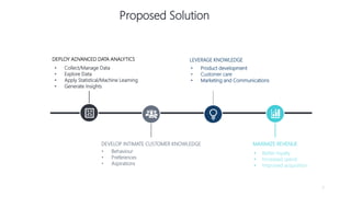
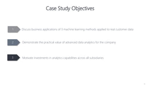
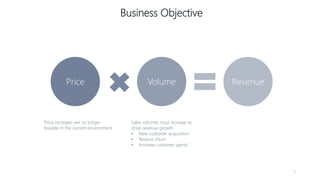
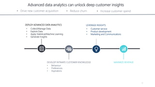


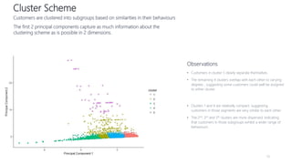
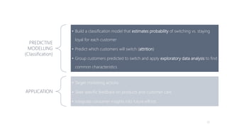
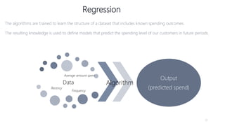
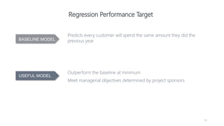
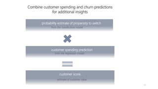
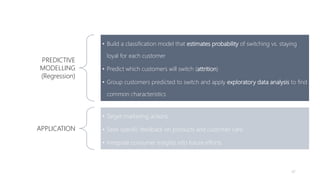


1) The document proposes using advanced data analytics to build knowledge of customer behavior, preferences, and aspirations in order to maximize revenue. 2) A case study uses data from an online beauty/personal care subsidiary to demonstrate how clustering, classification, and regression analyses can provide insights. 3) The analyses identify customer subgroups, predict which customers will churn, and forecast spending amounts. This knowledge can then be used to target marketing and improve customer retention and spending.


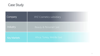
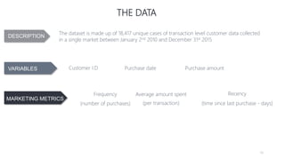
![New Customer Acquisition Presentation[1]](https://cdn.slidesharecdn.com/ss_thumbnails/newcustomeracquisitionpresentation1-12699987508146-phpapp02-thumbnail.jpg?width=640&height=640&fit=bounds)


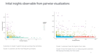
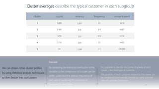
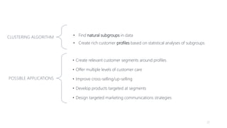
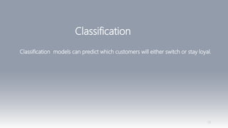
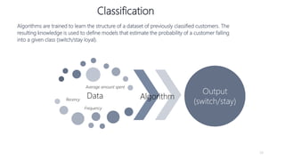
![Cdac -Project Presentation [Autosaved].pptx](https://cdn.slidesharecdn.com/ss_thumbnails/cdac-projectpresentationautosaved-231029063336-13e0f780-thumbnail.jpg?width=640&height=640&fit=bounds)


![[DSC Europe 25] Andrzej Kowalczyk - AI - how to start small and grow in the f...](https://cdn.slidesharecdn.com/ss_thumbnails/oy1zmo94qv6vpcqjvno2-andrzej-kowalczyk-ai-how-to-start-small-and-grow-in-the-future-1-260119121559-cf093b23-thumbnail.jpg?width=640&height=640&fit=bounds)


![[DSC Europe 25] Bojan Djuricic - Predictive Design Process.pdf](https://cdn.slidesharecdn.com/ss_thumbnails/5awdrbedqdek3gqu2ezy-4-the-predictive-design-bojan-djuricic-260120105856-6c399e9b-thumbnail.jpg?width=640&height=640&fit=bounds)


