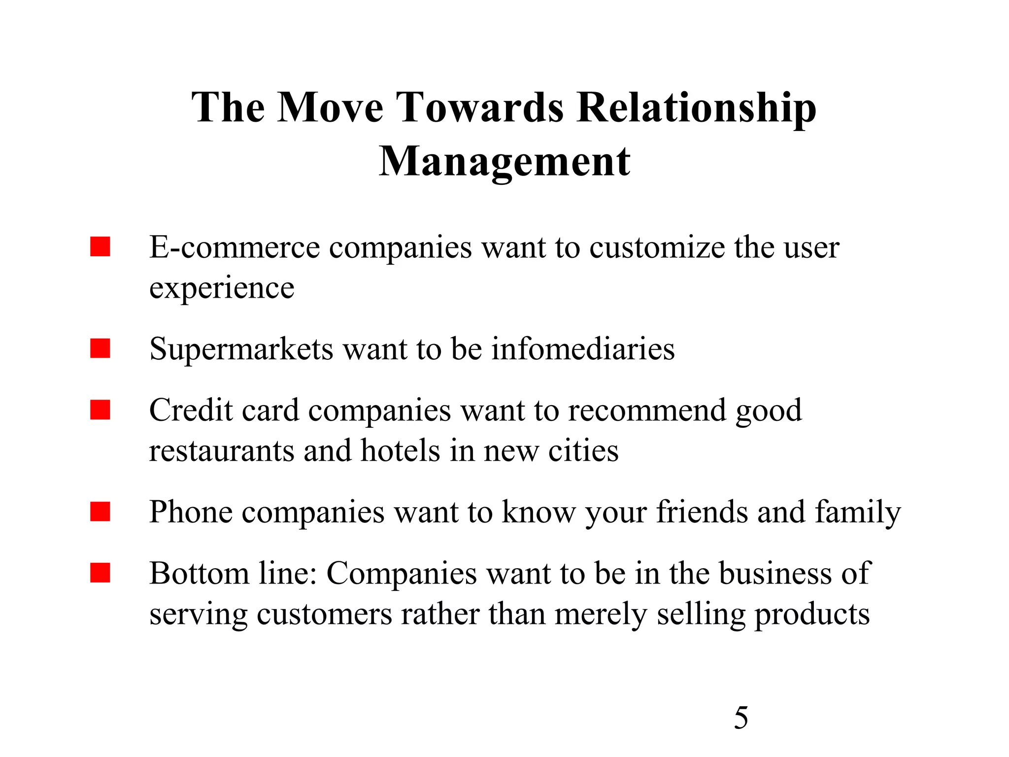
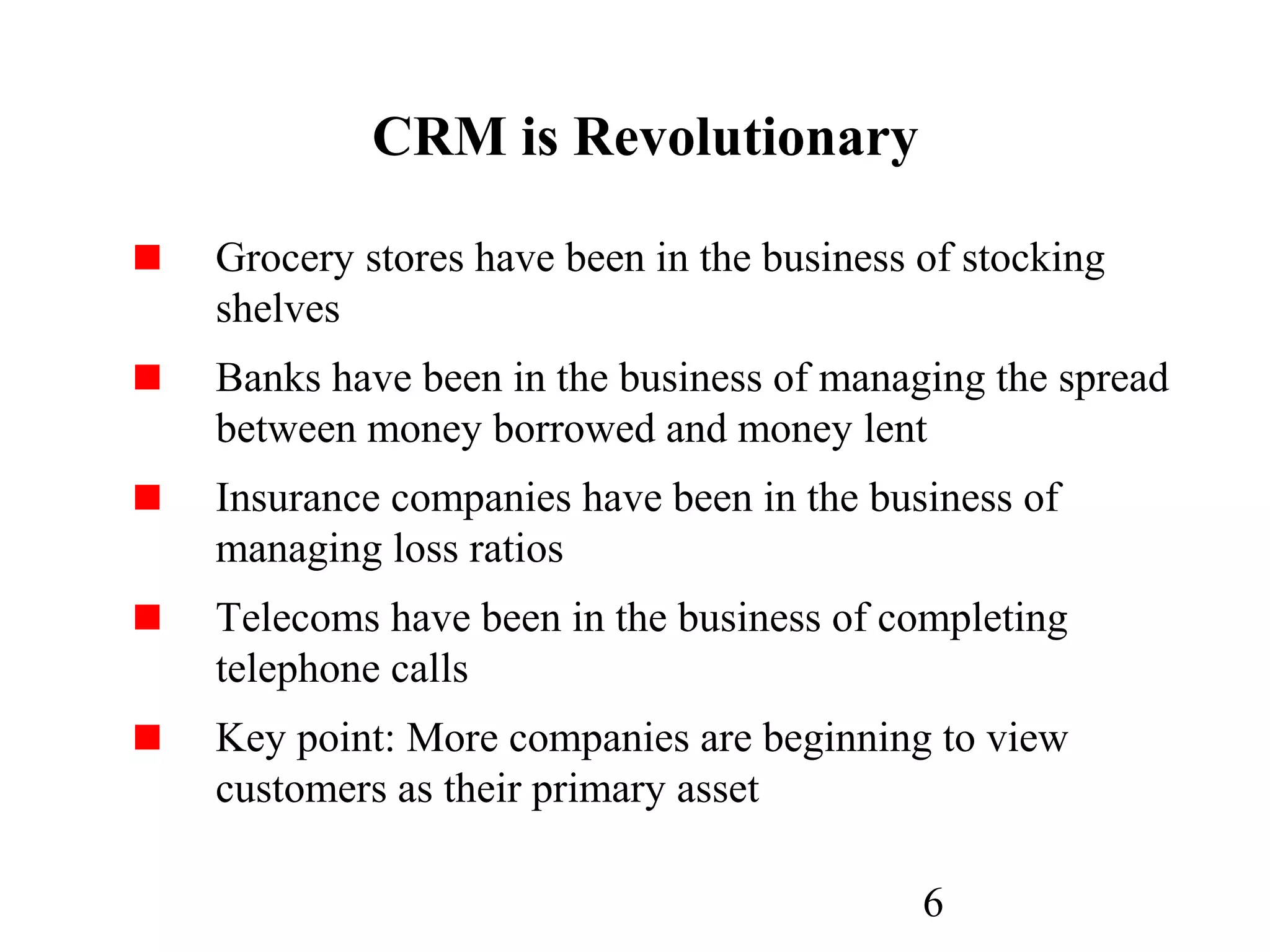
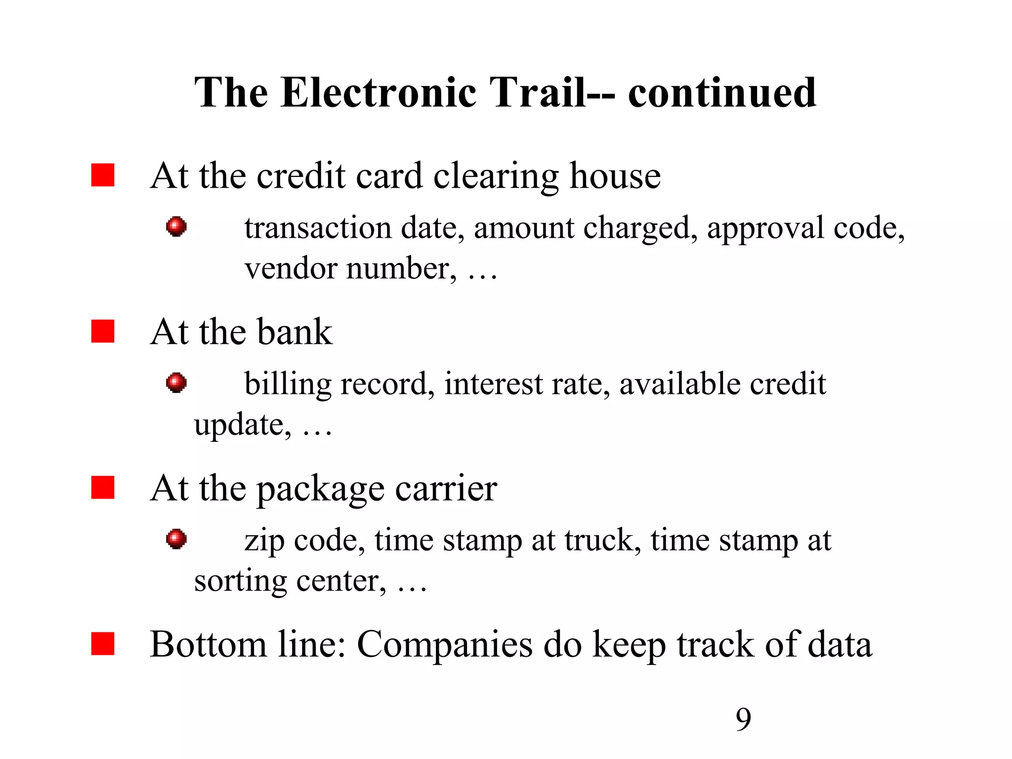
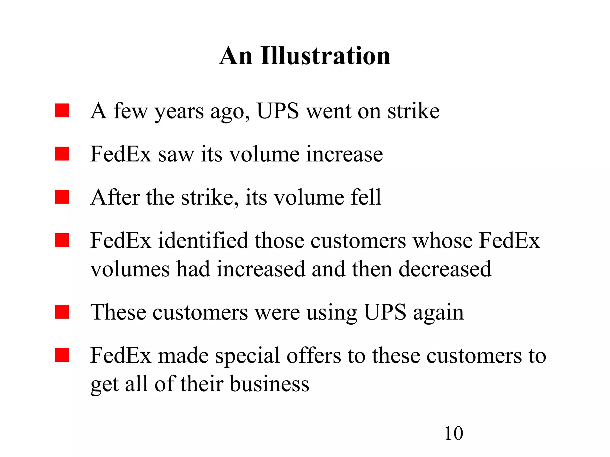
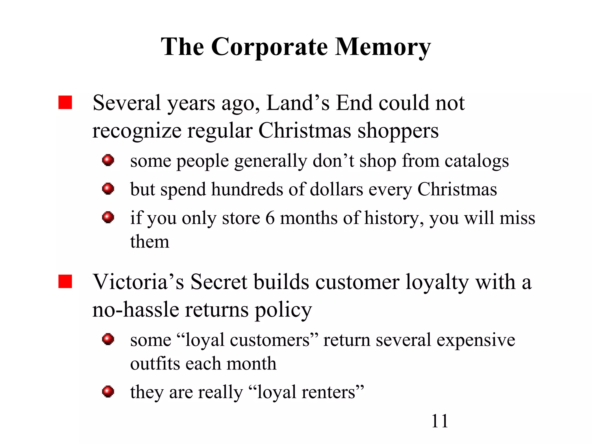
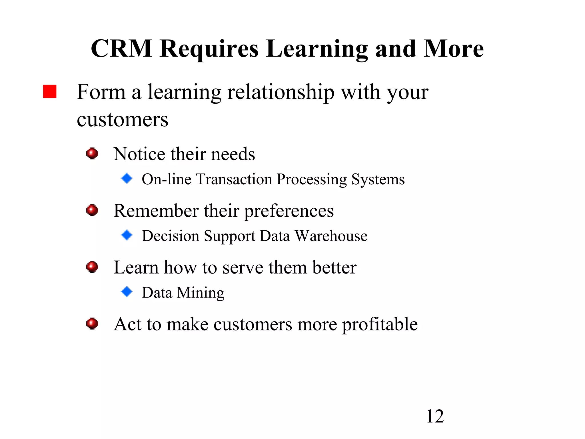
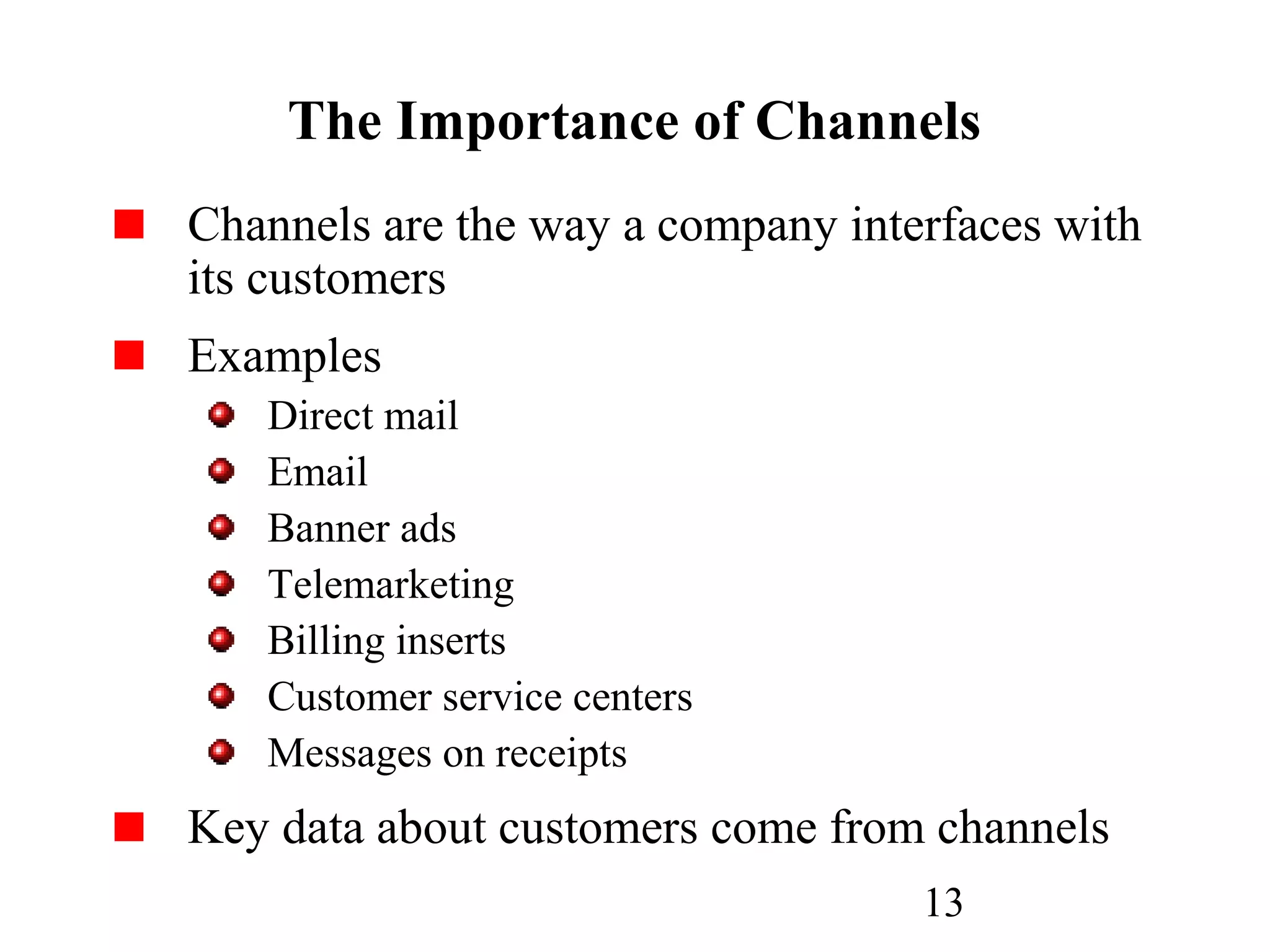
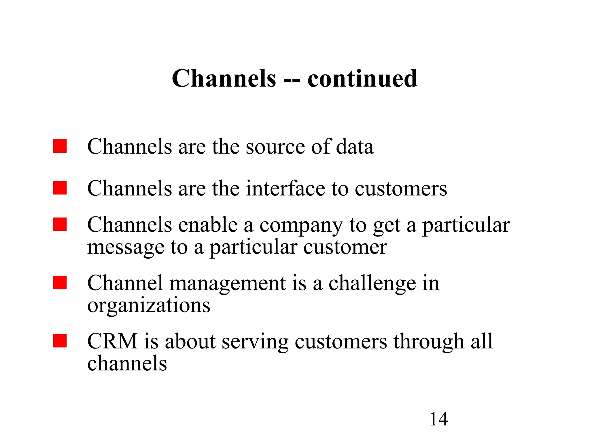
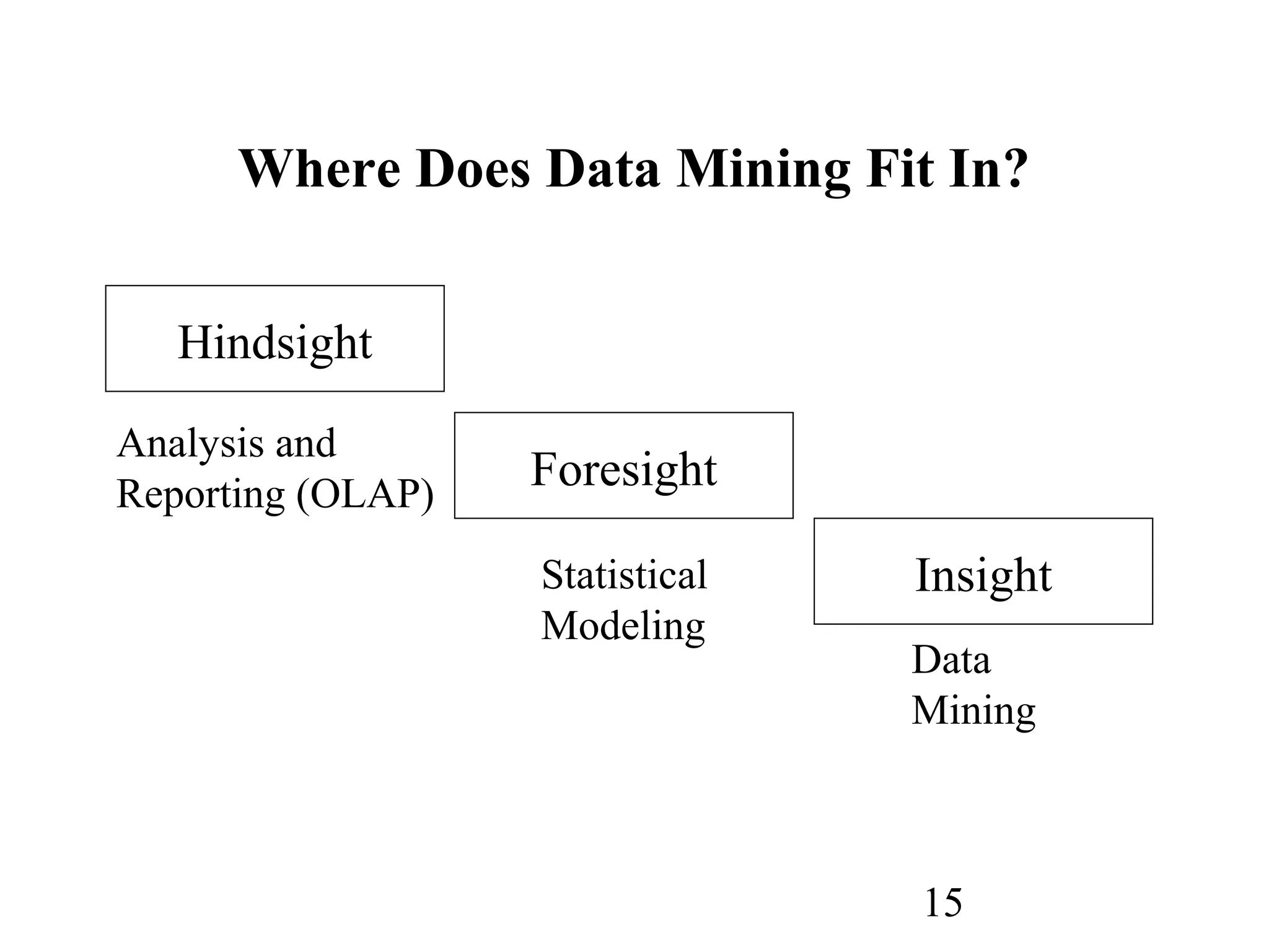
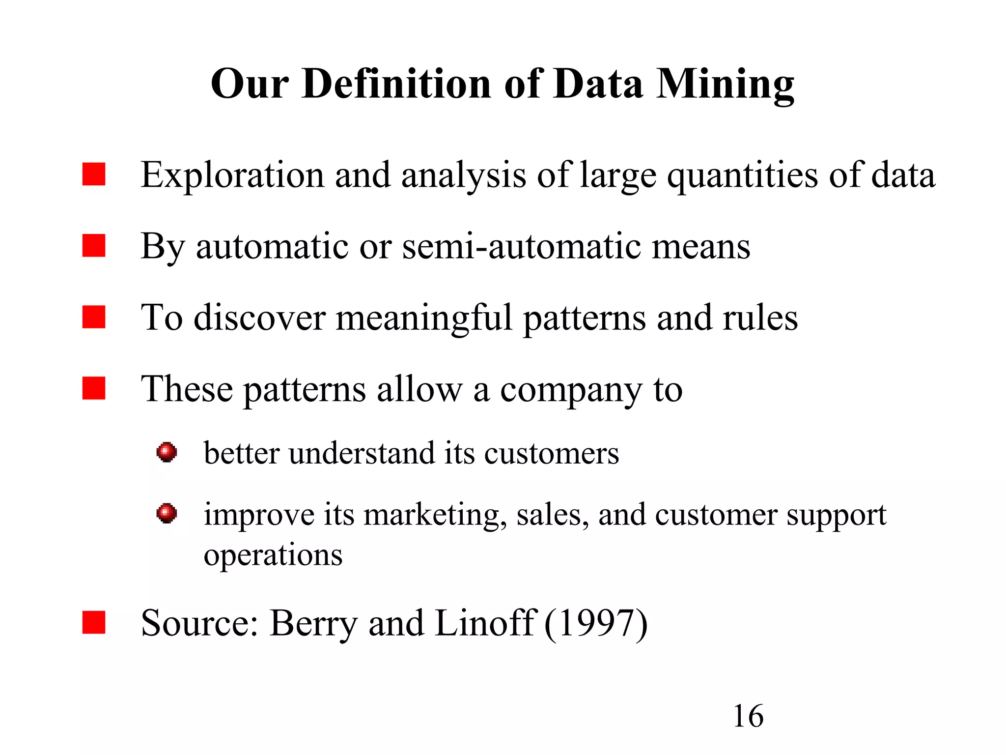
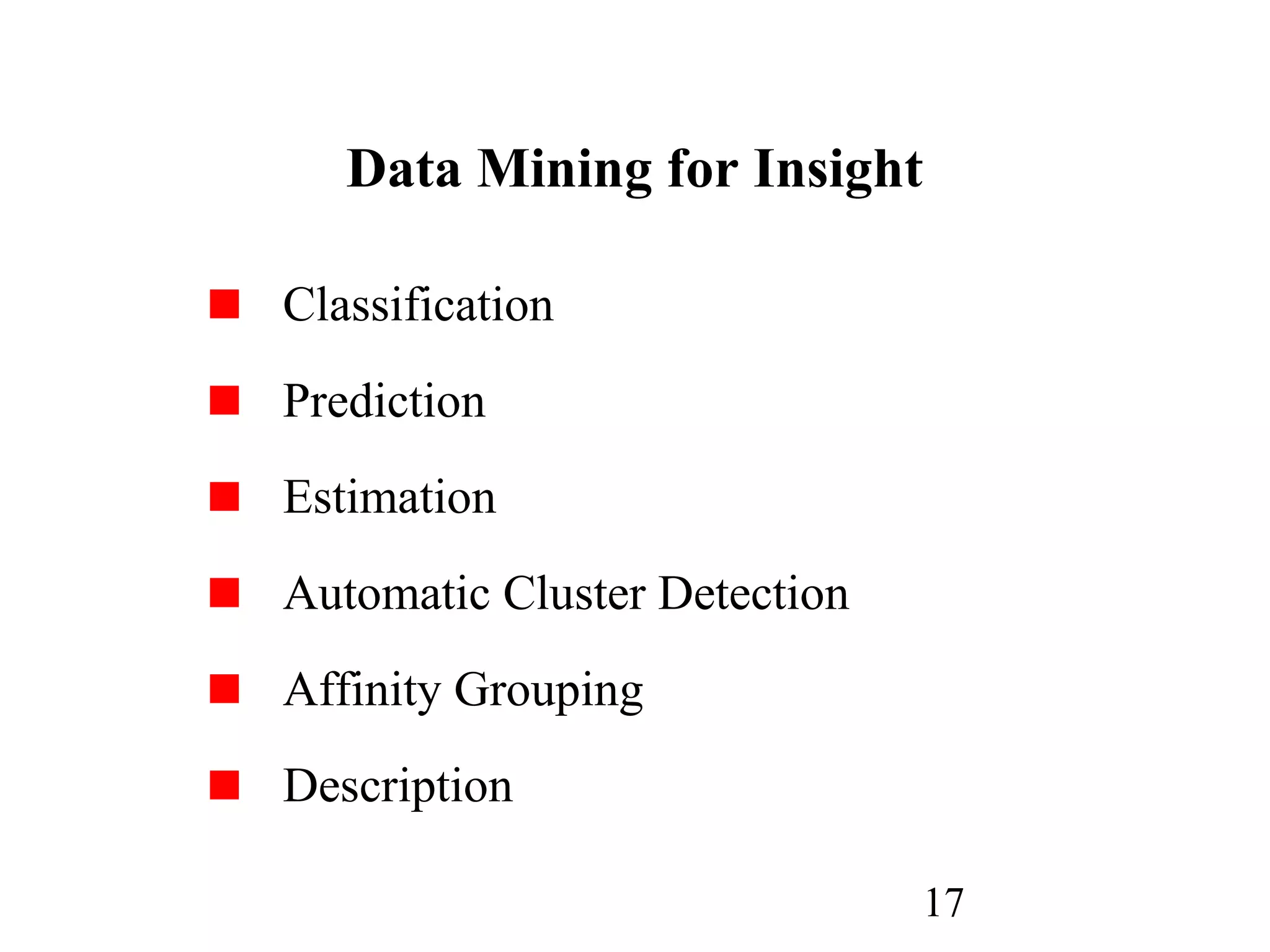
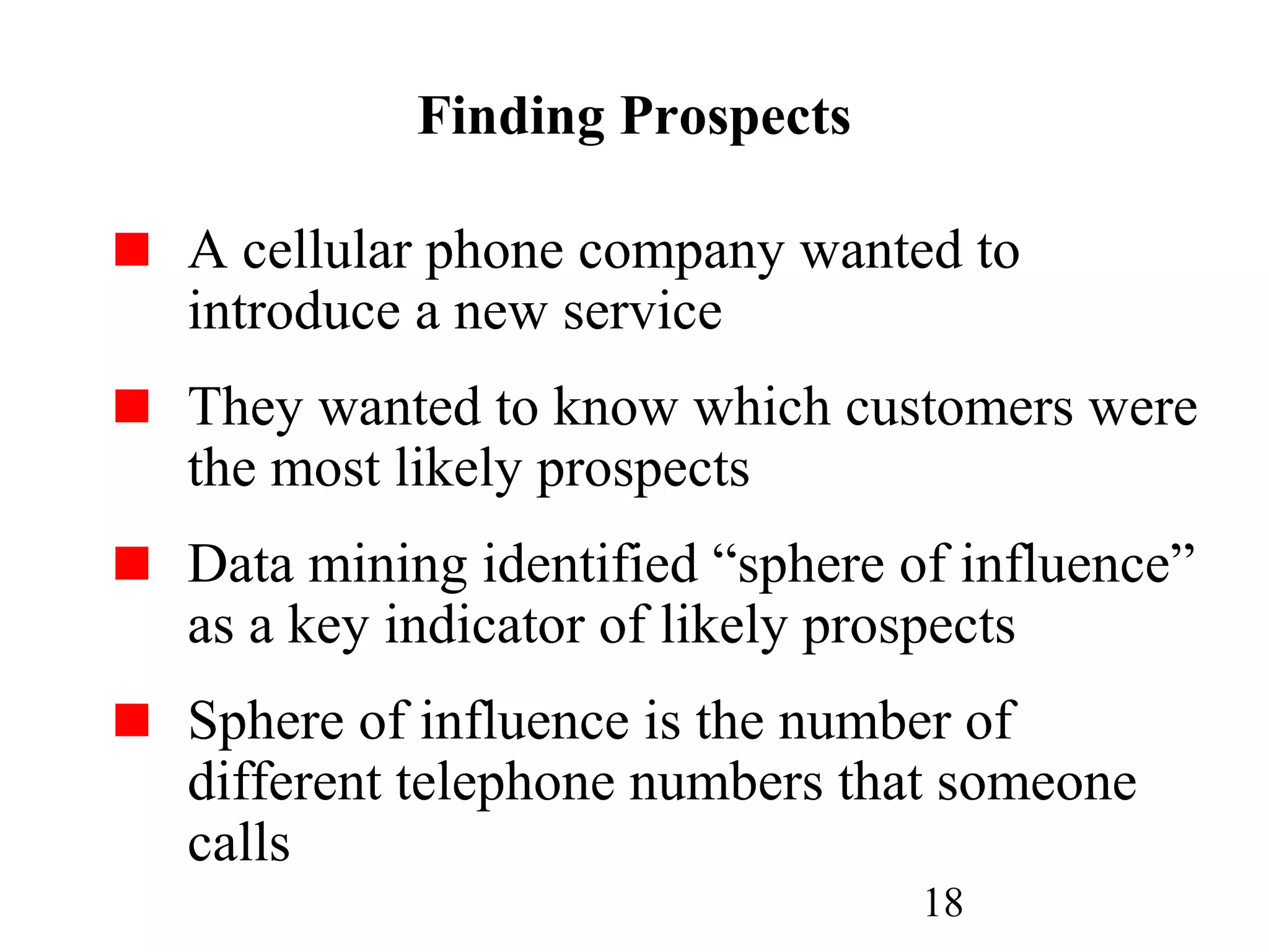
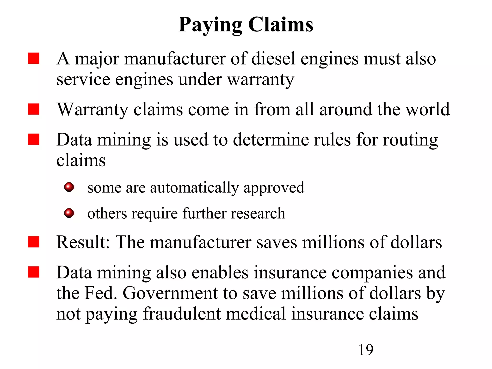
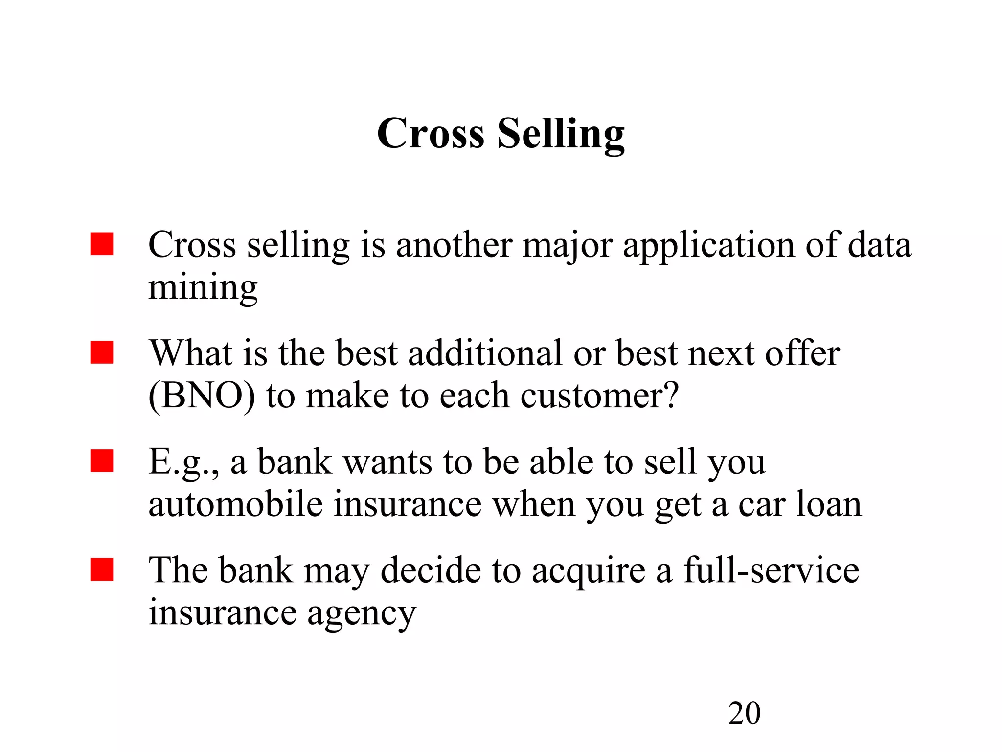
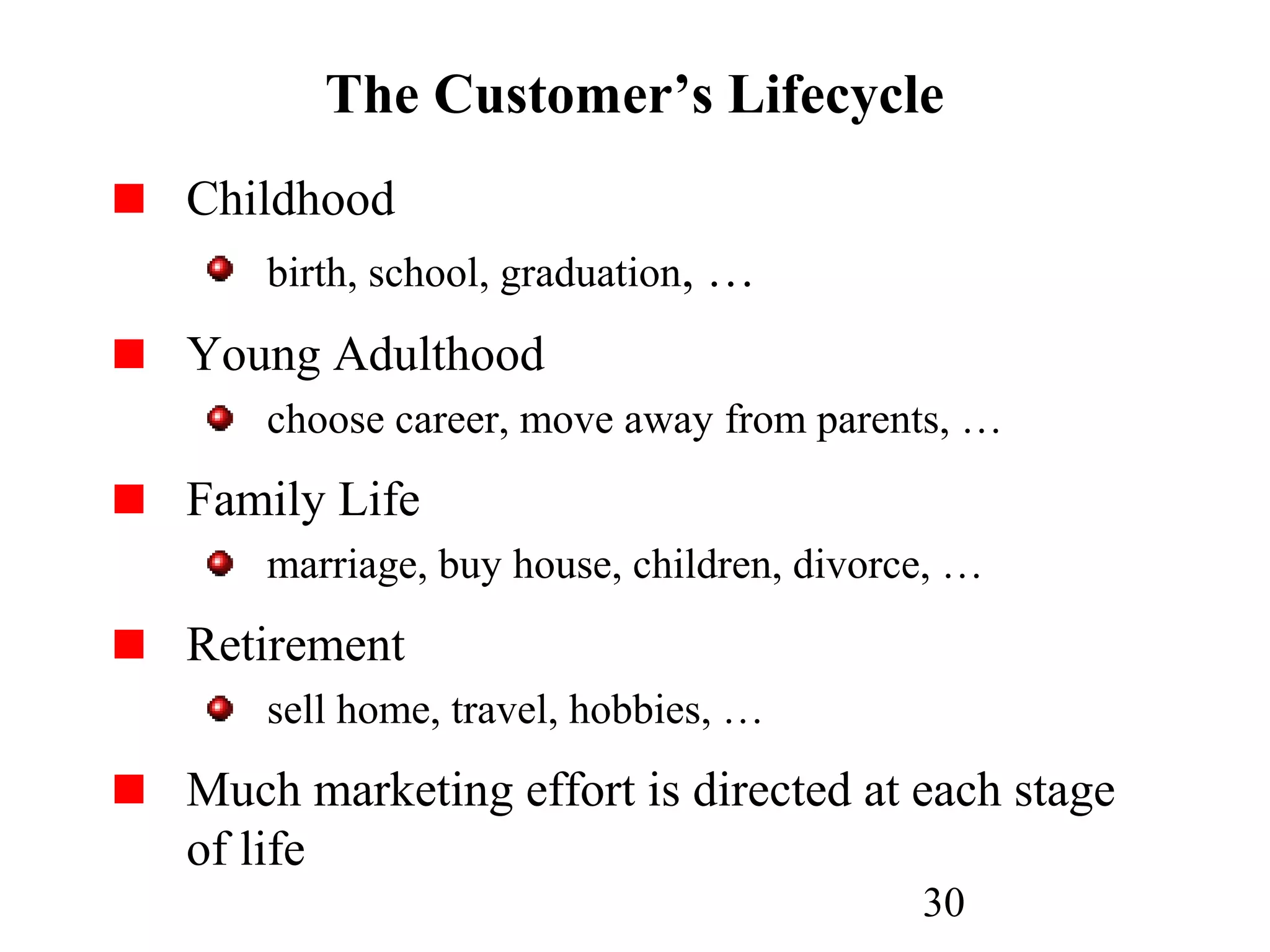
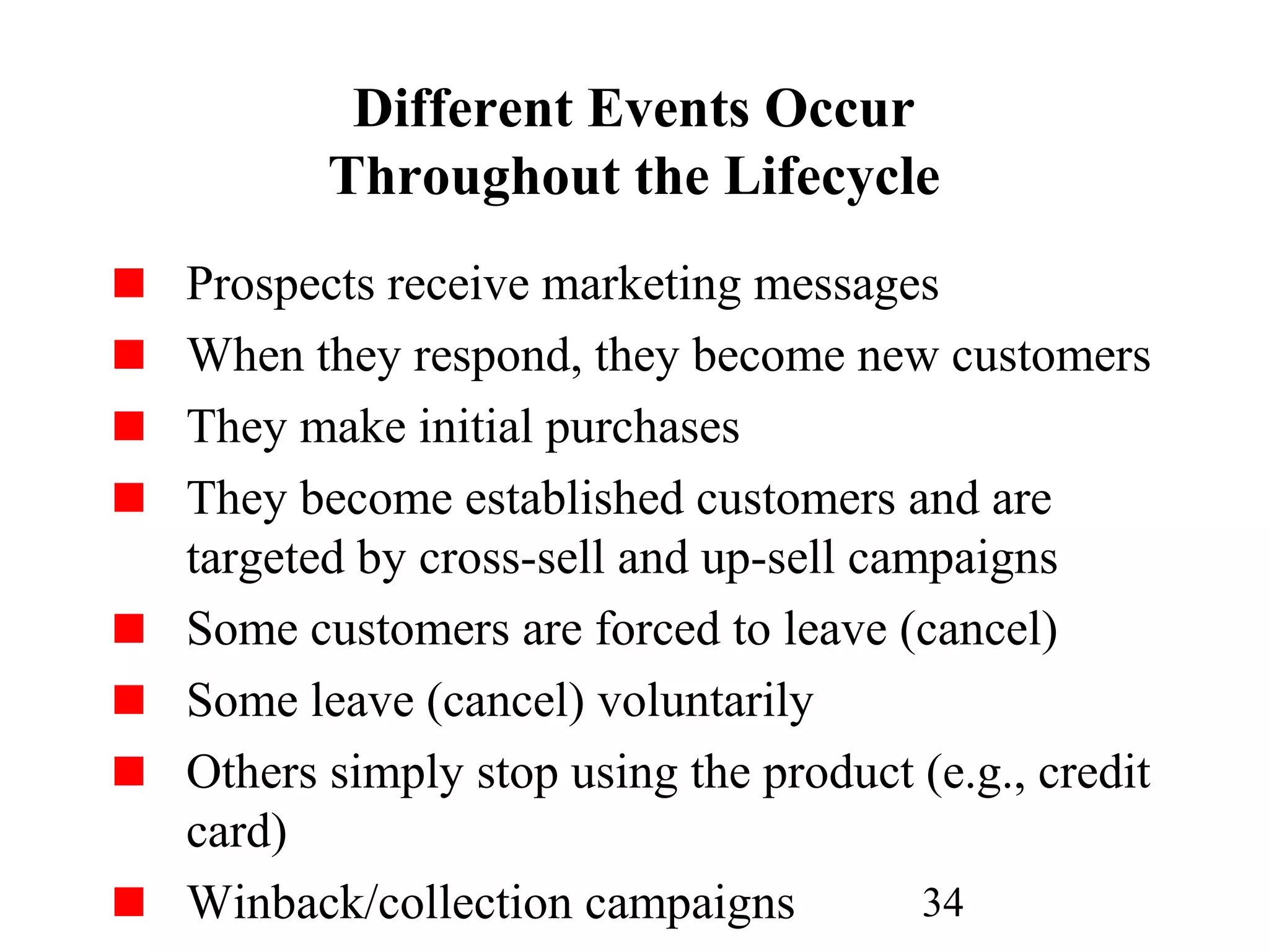
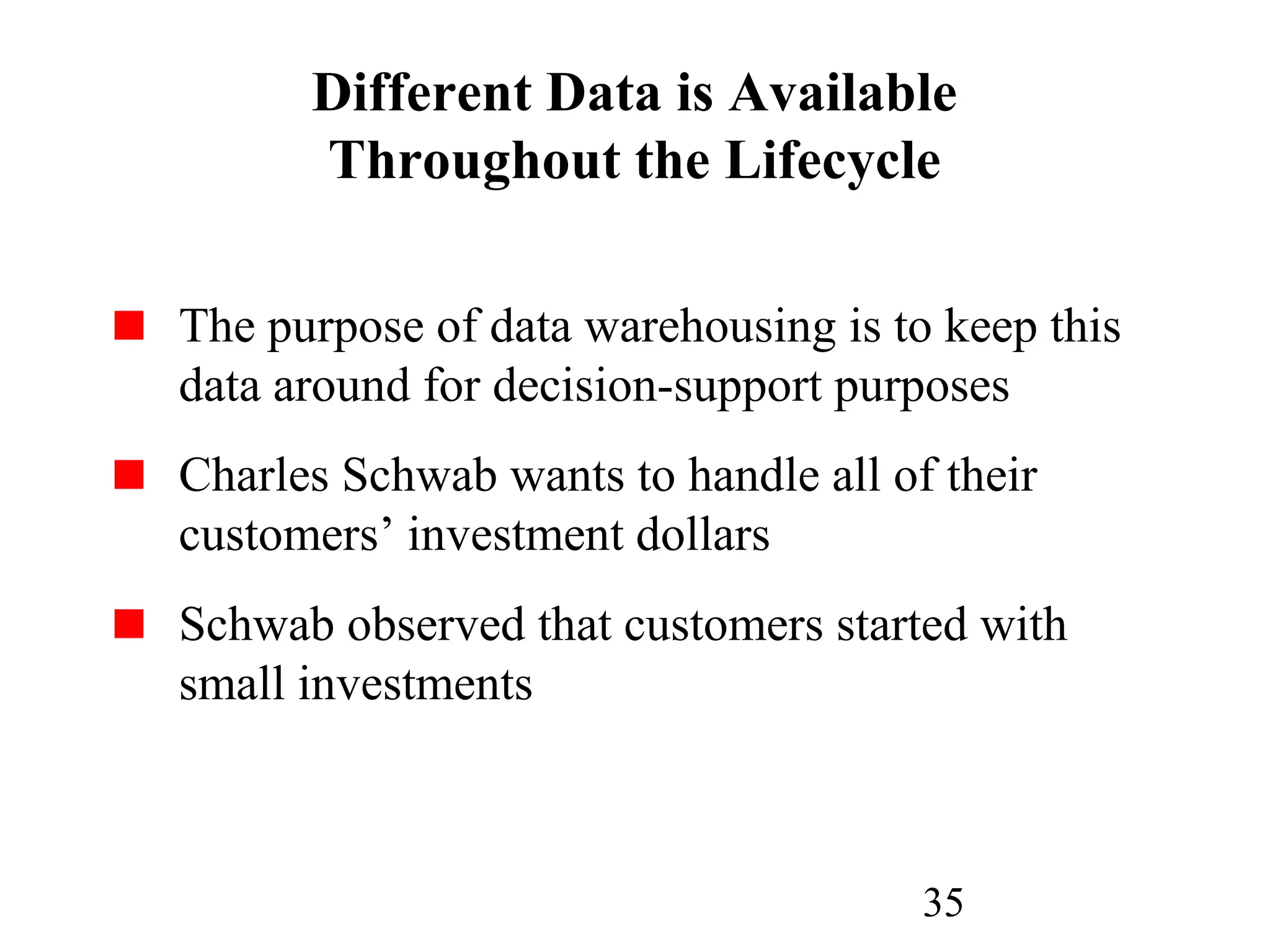
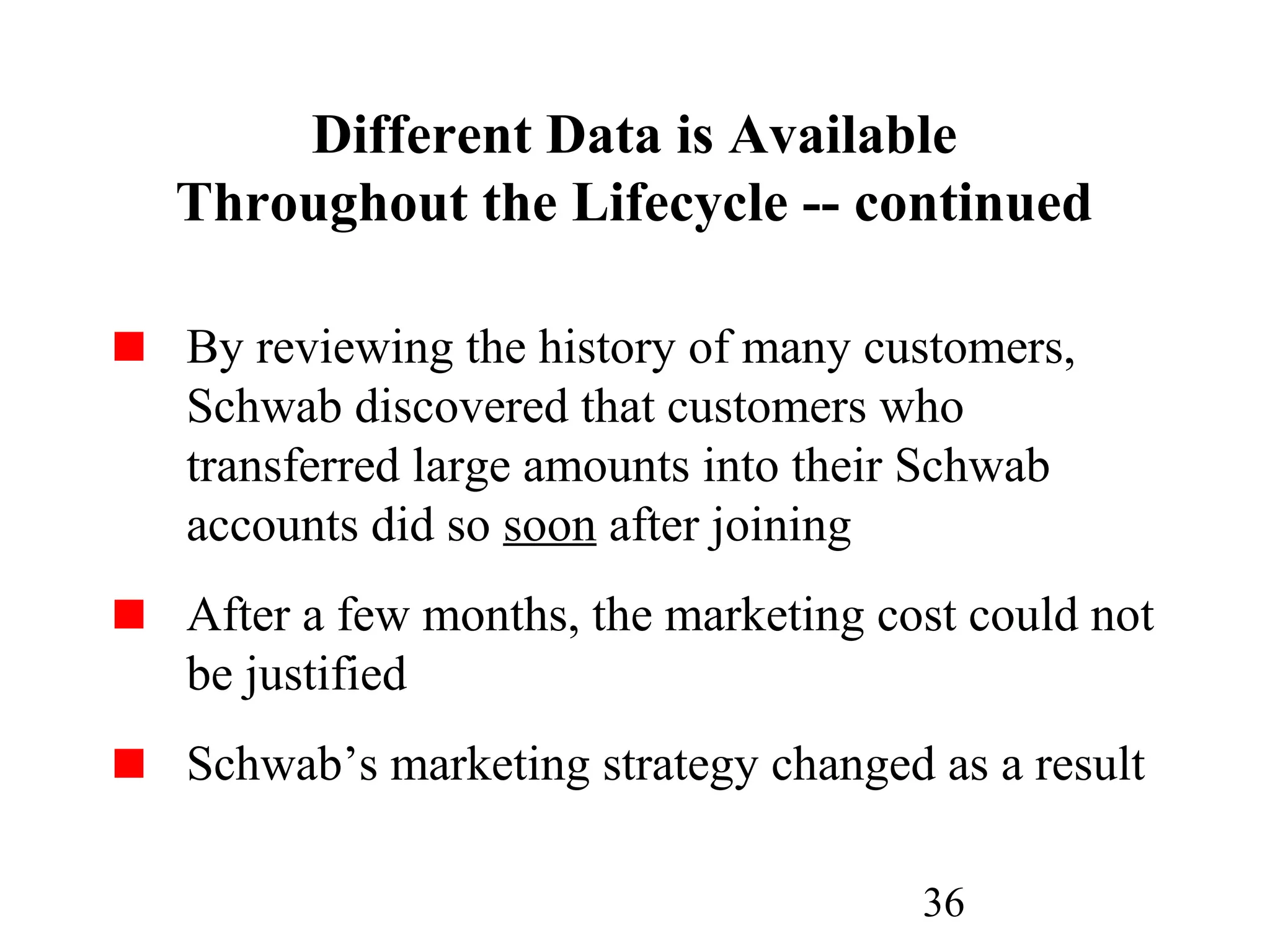
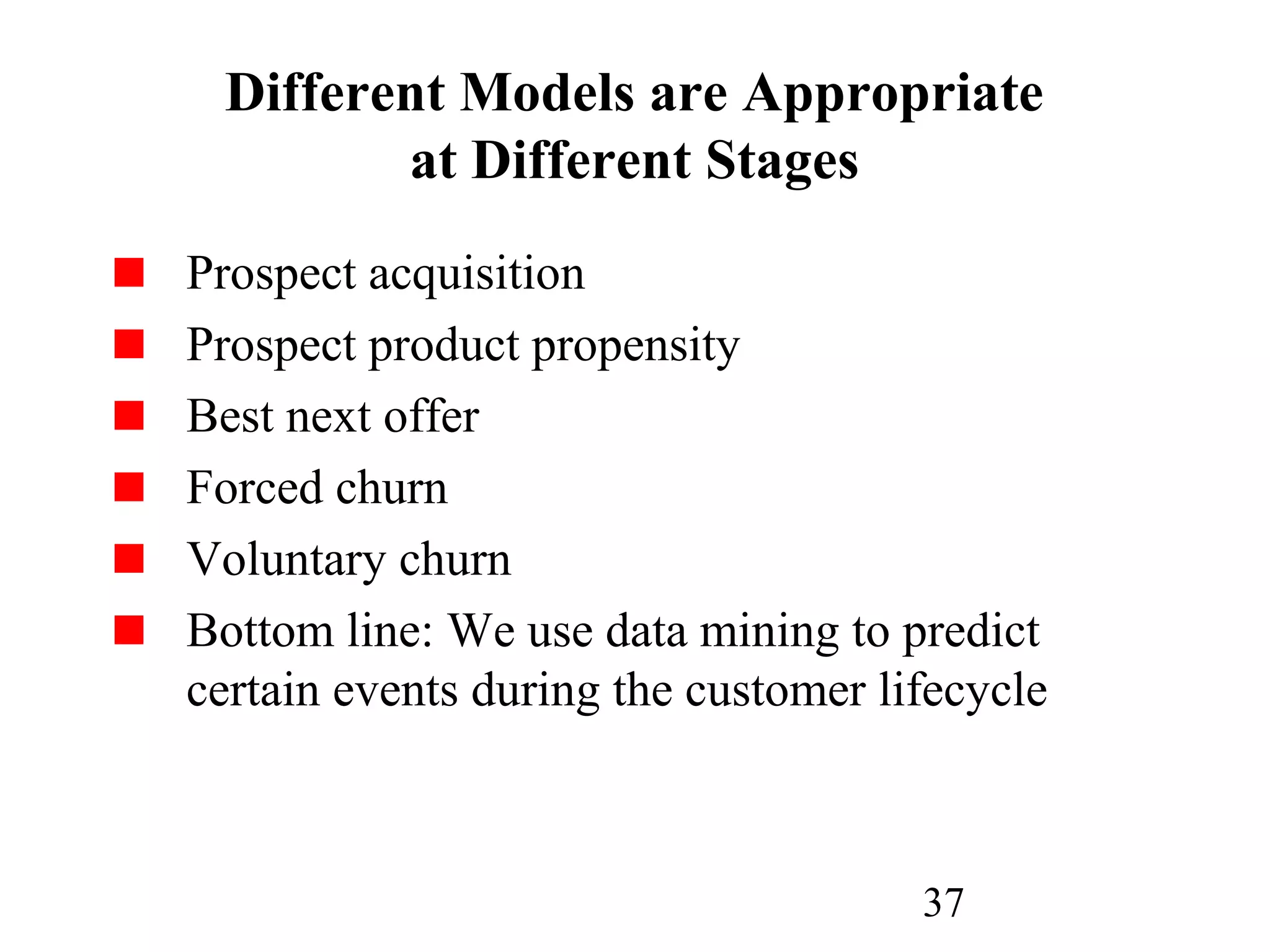
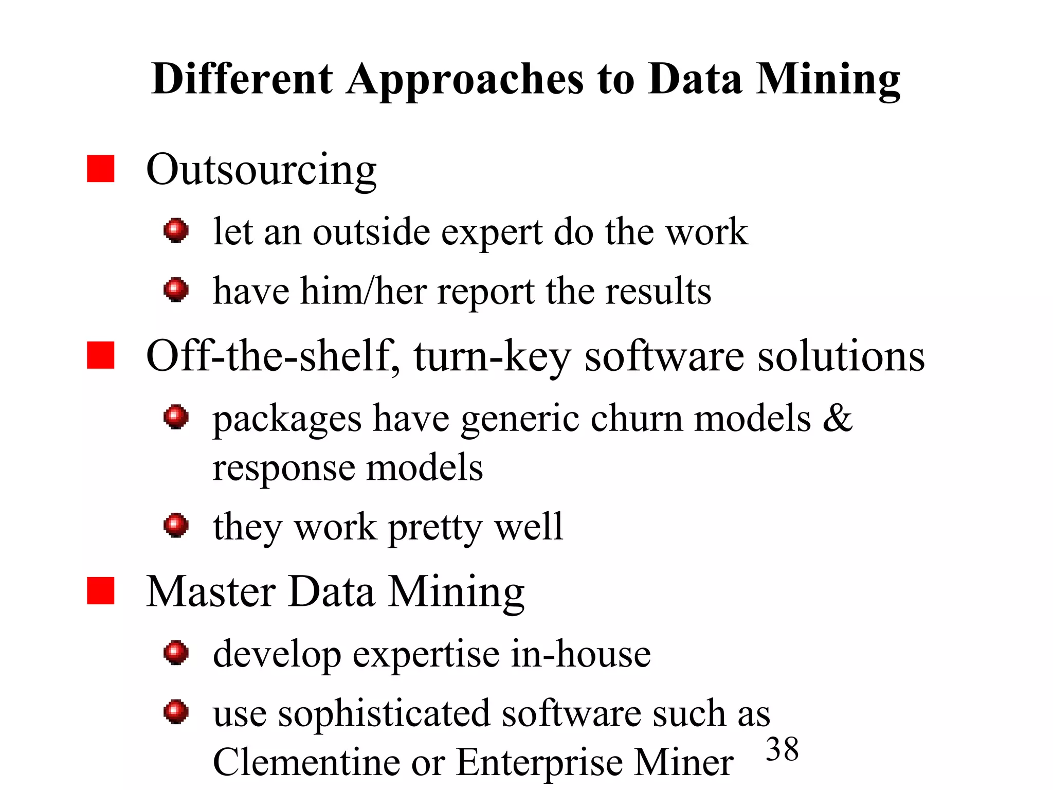
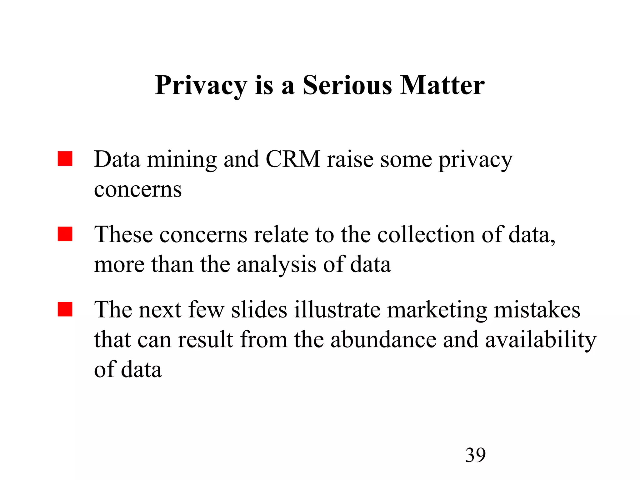
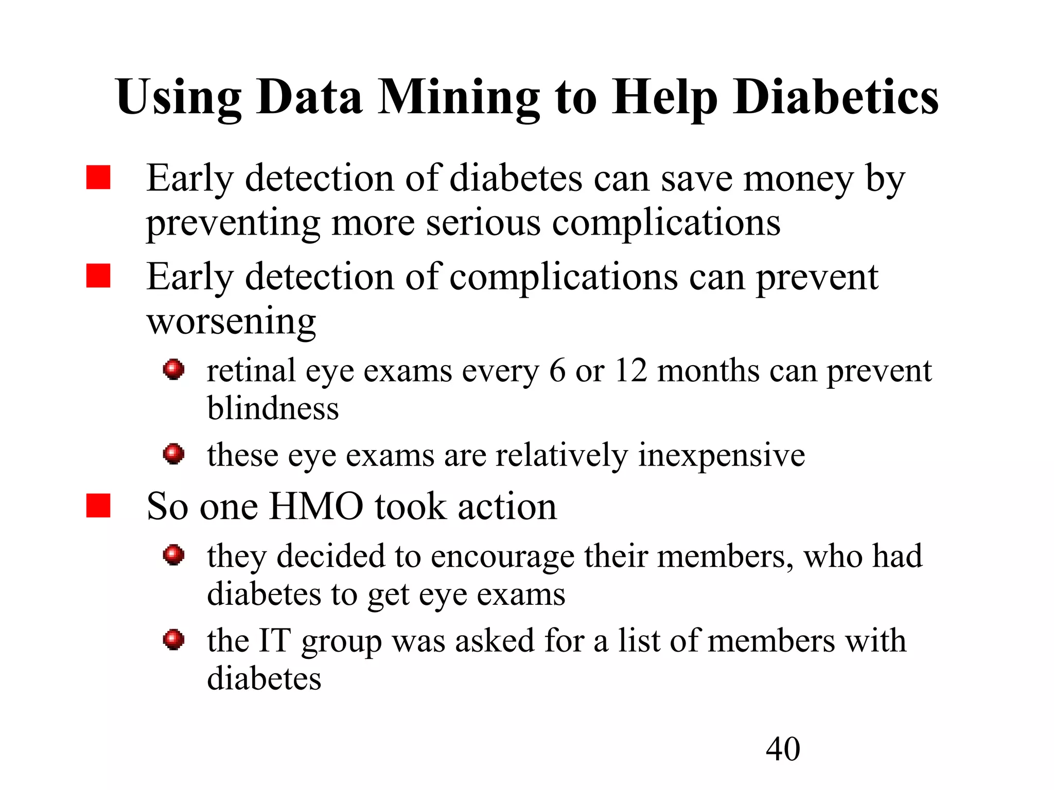
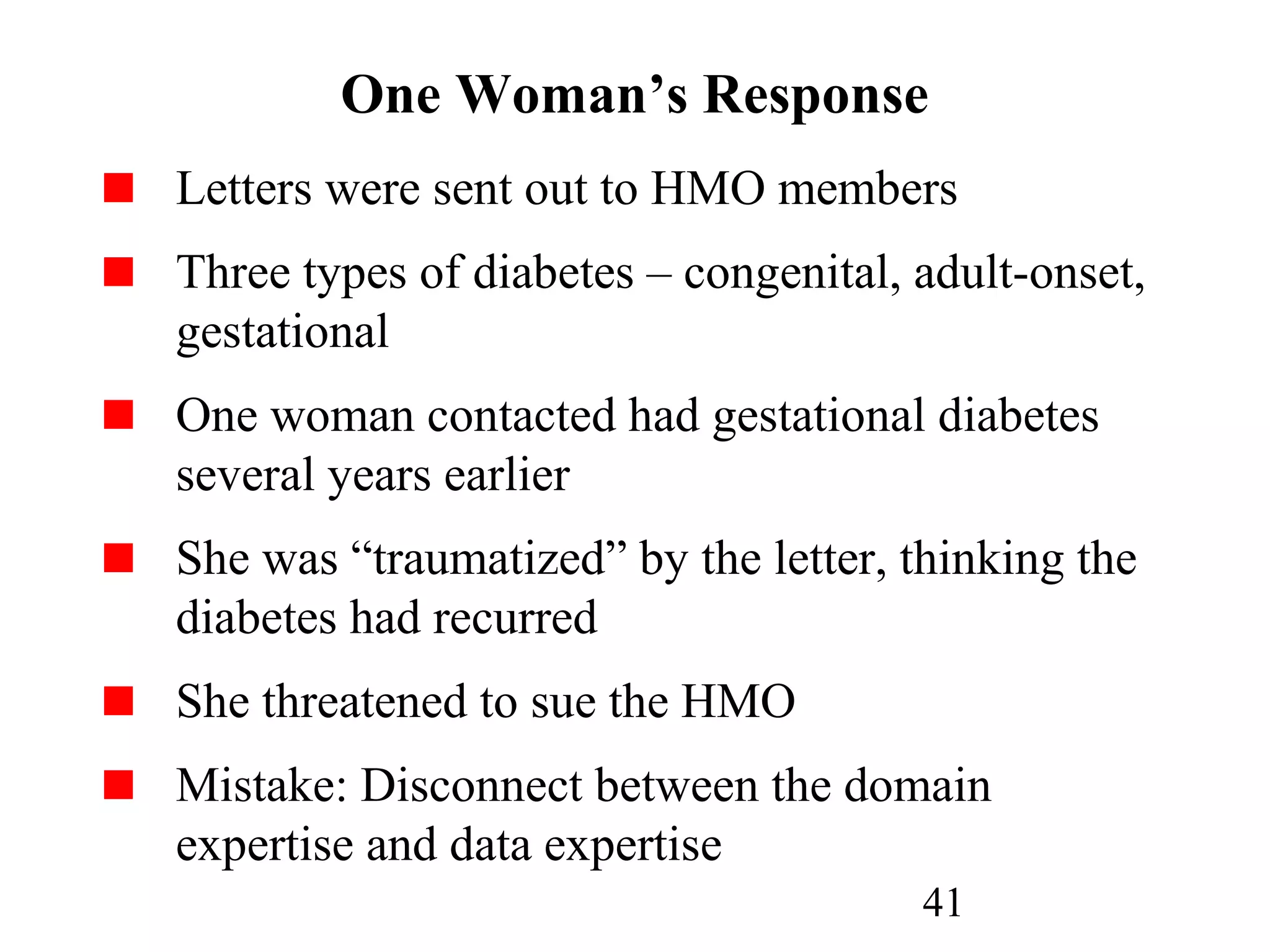
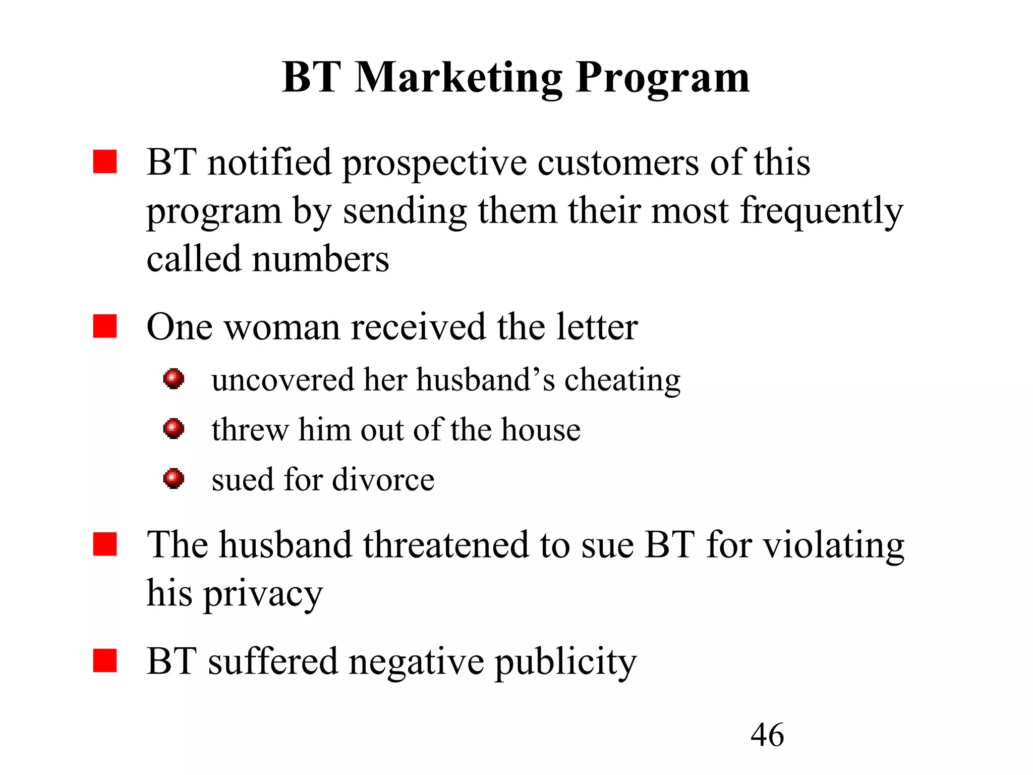
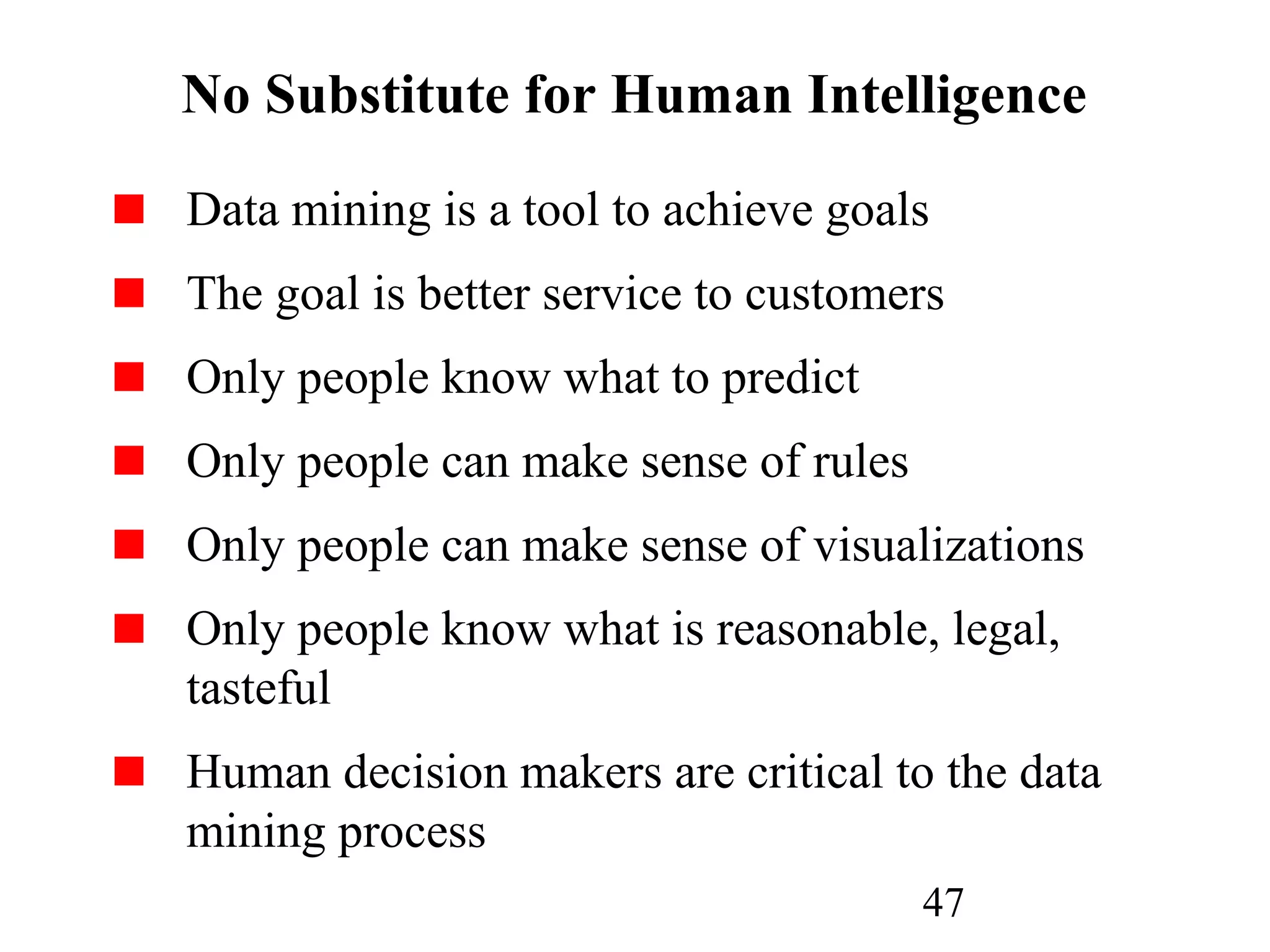
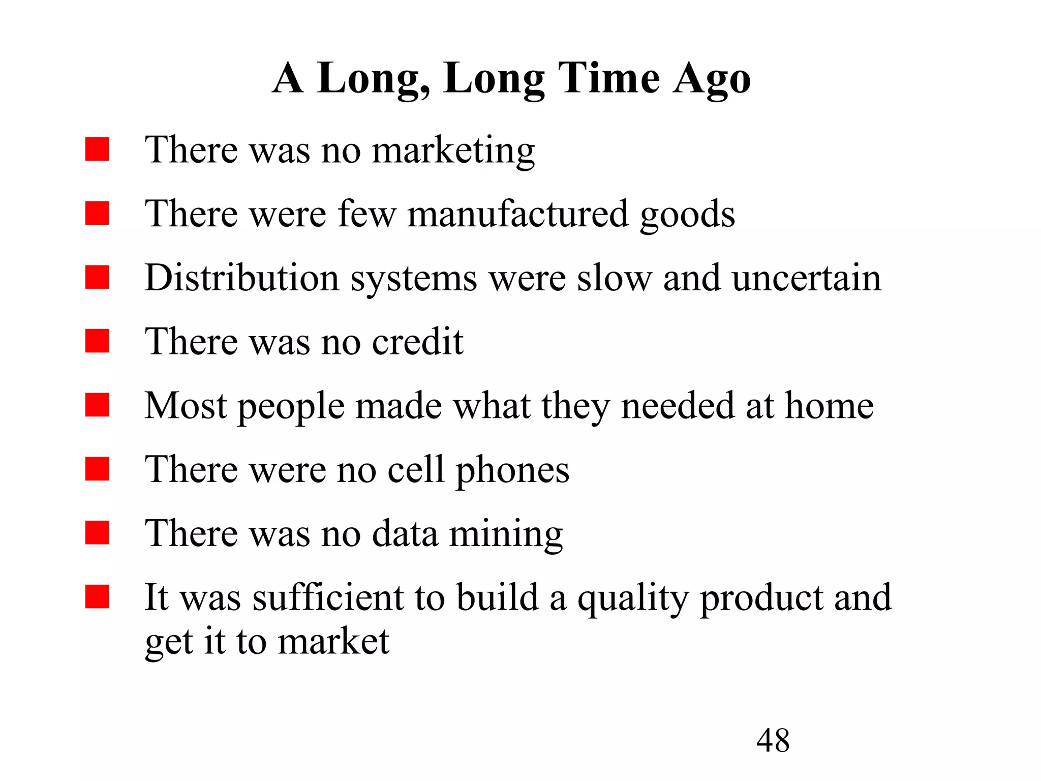
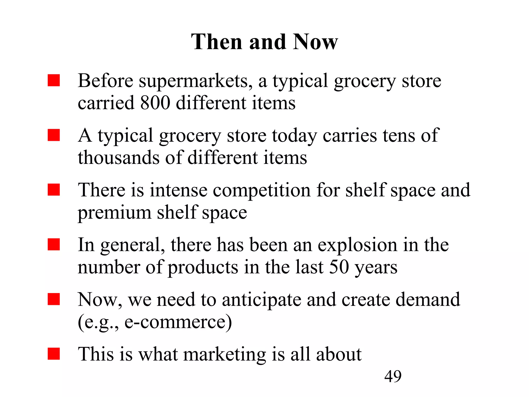
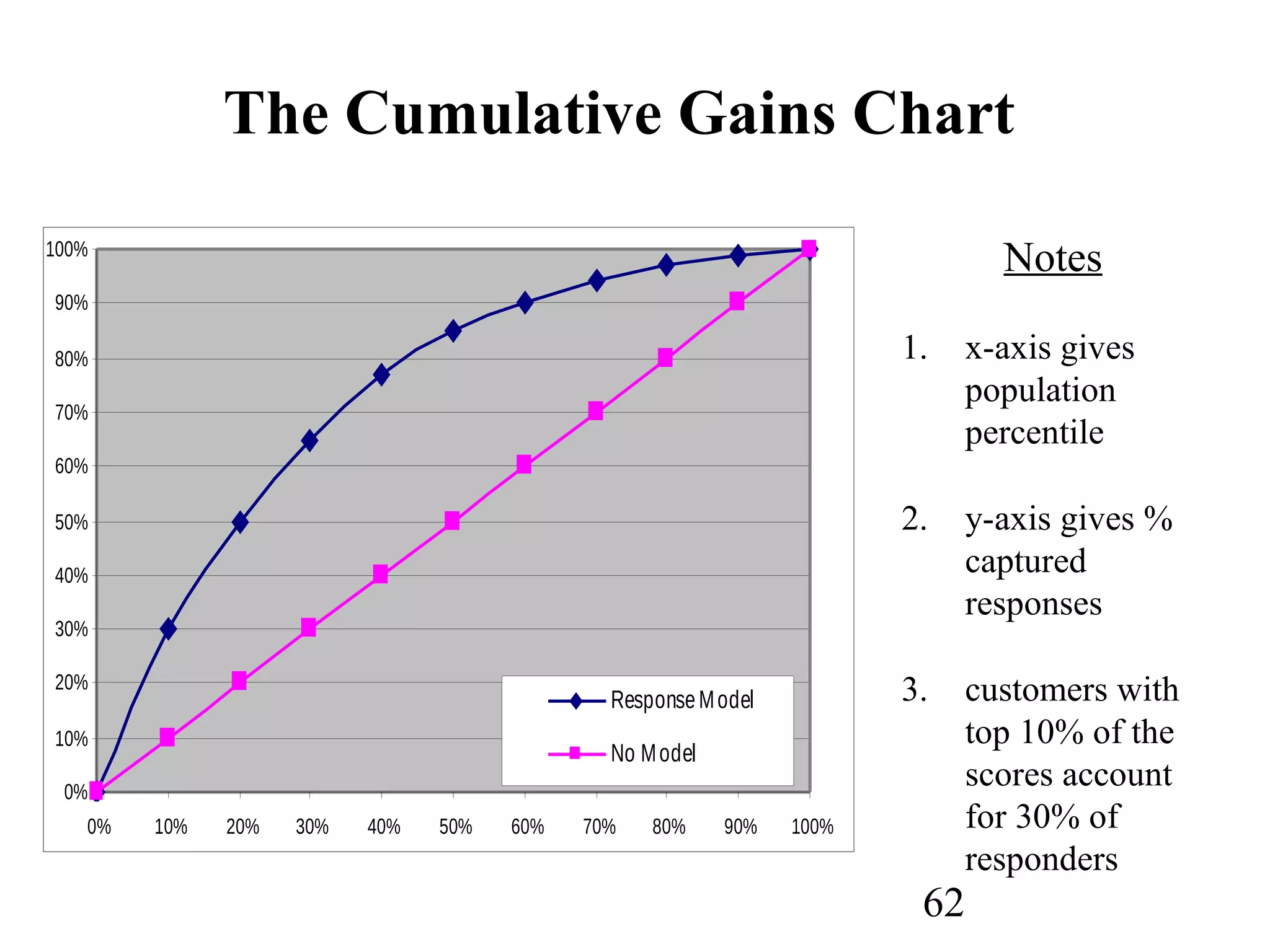
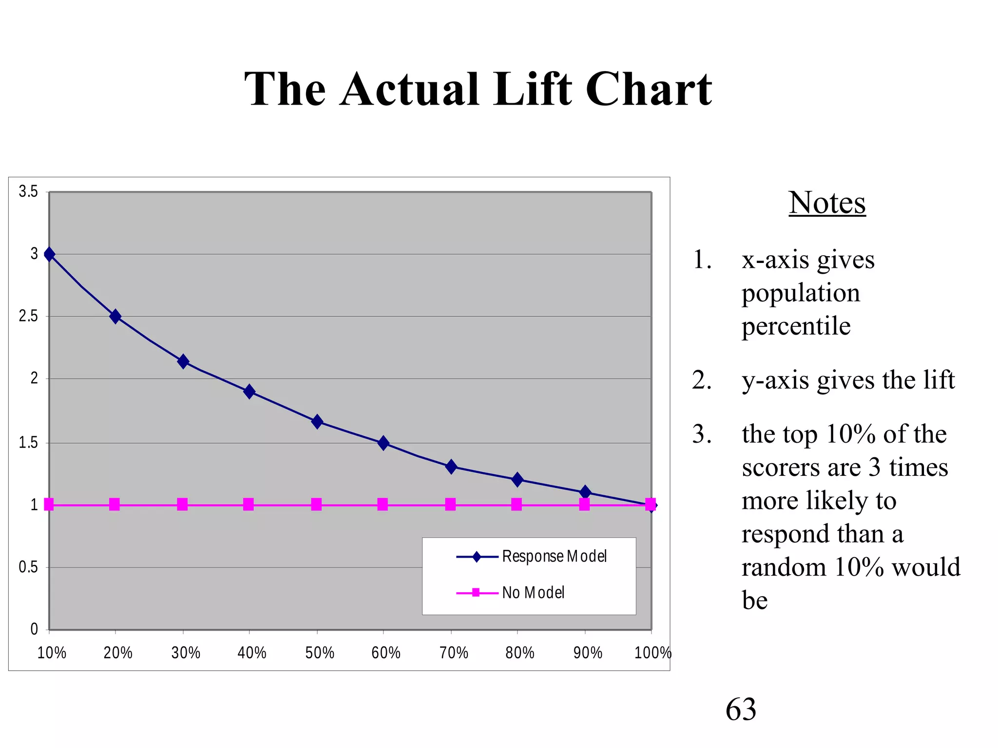
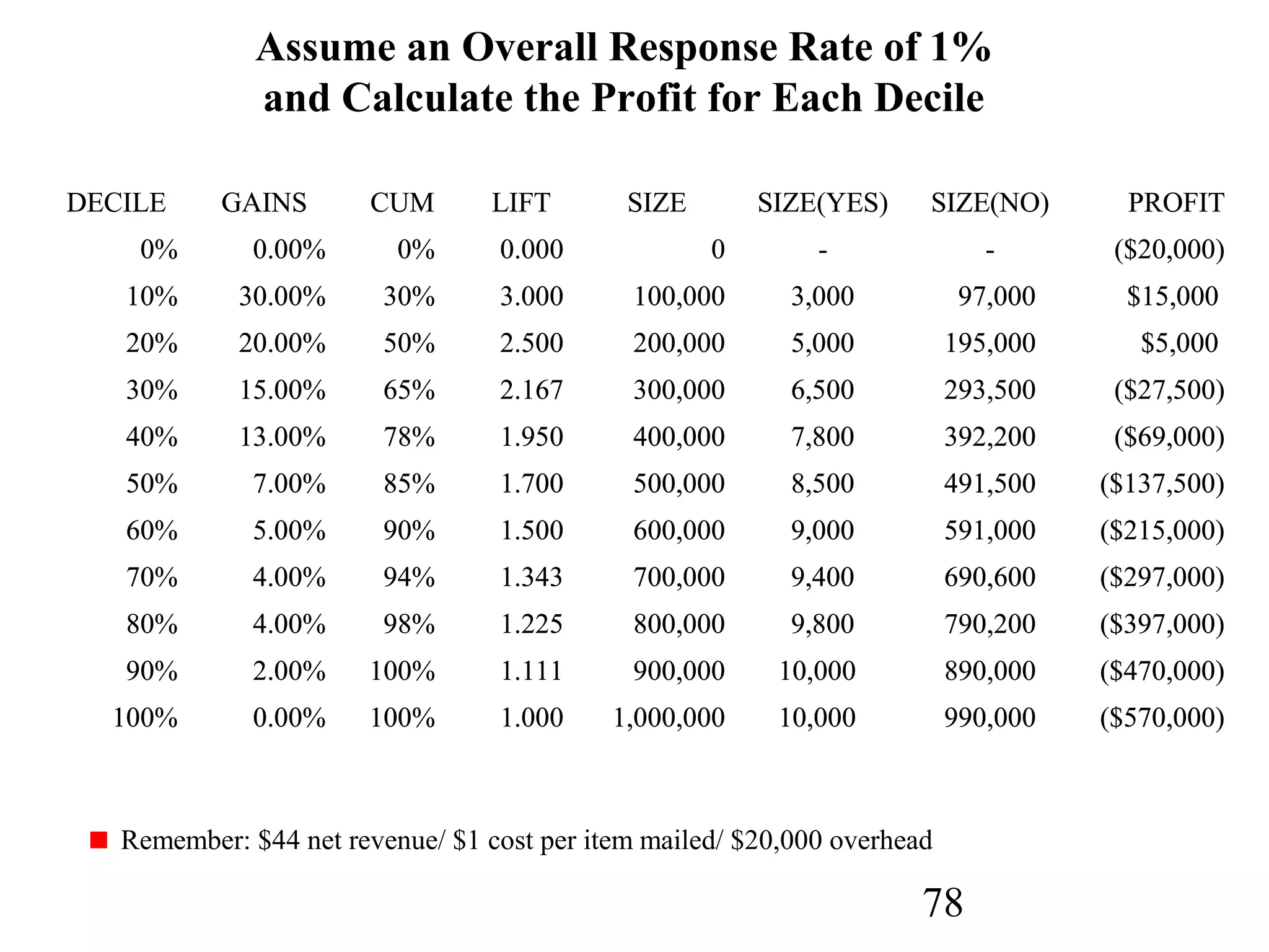
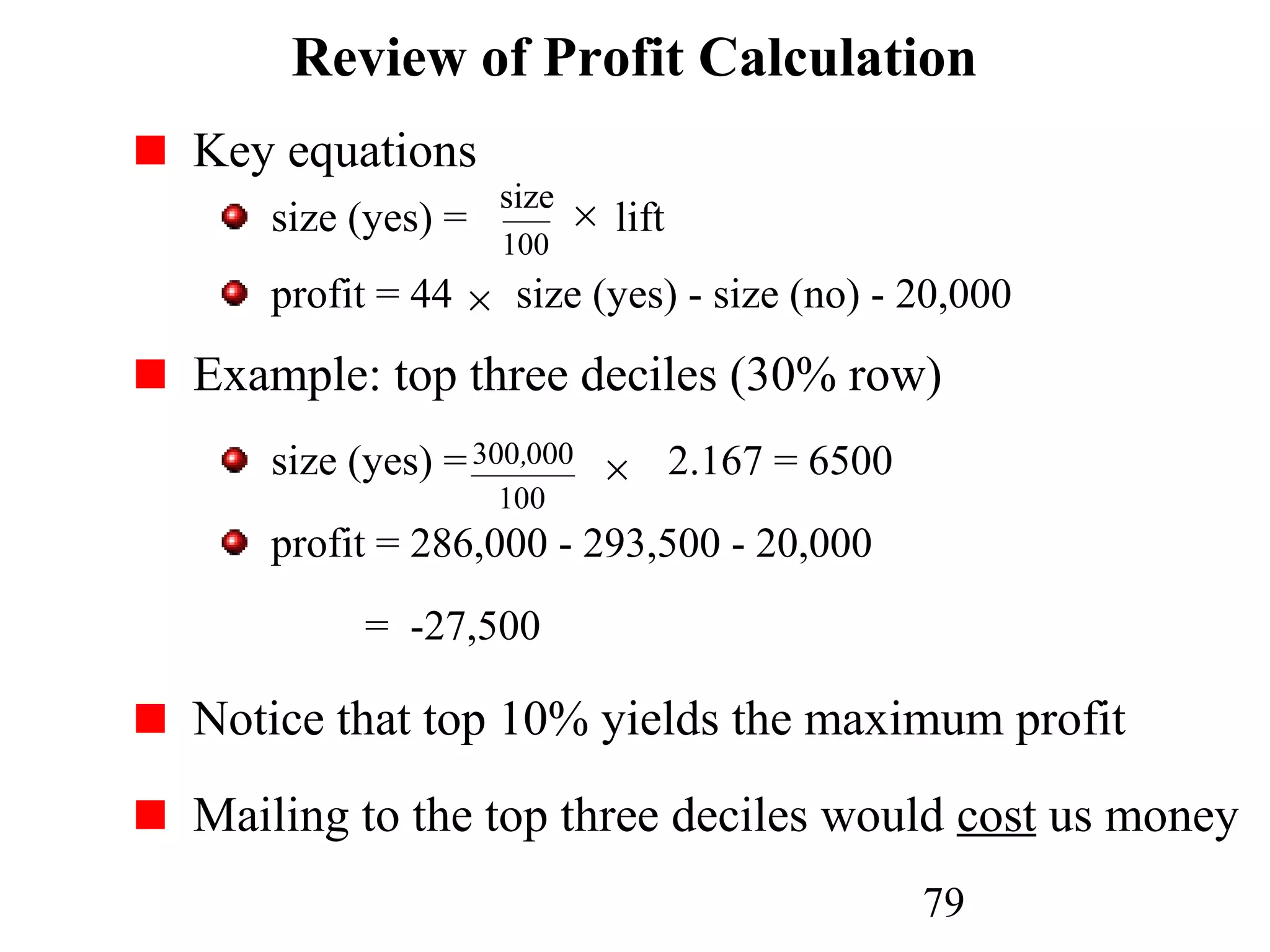
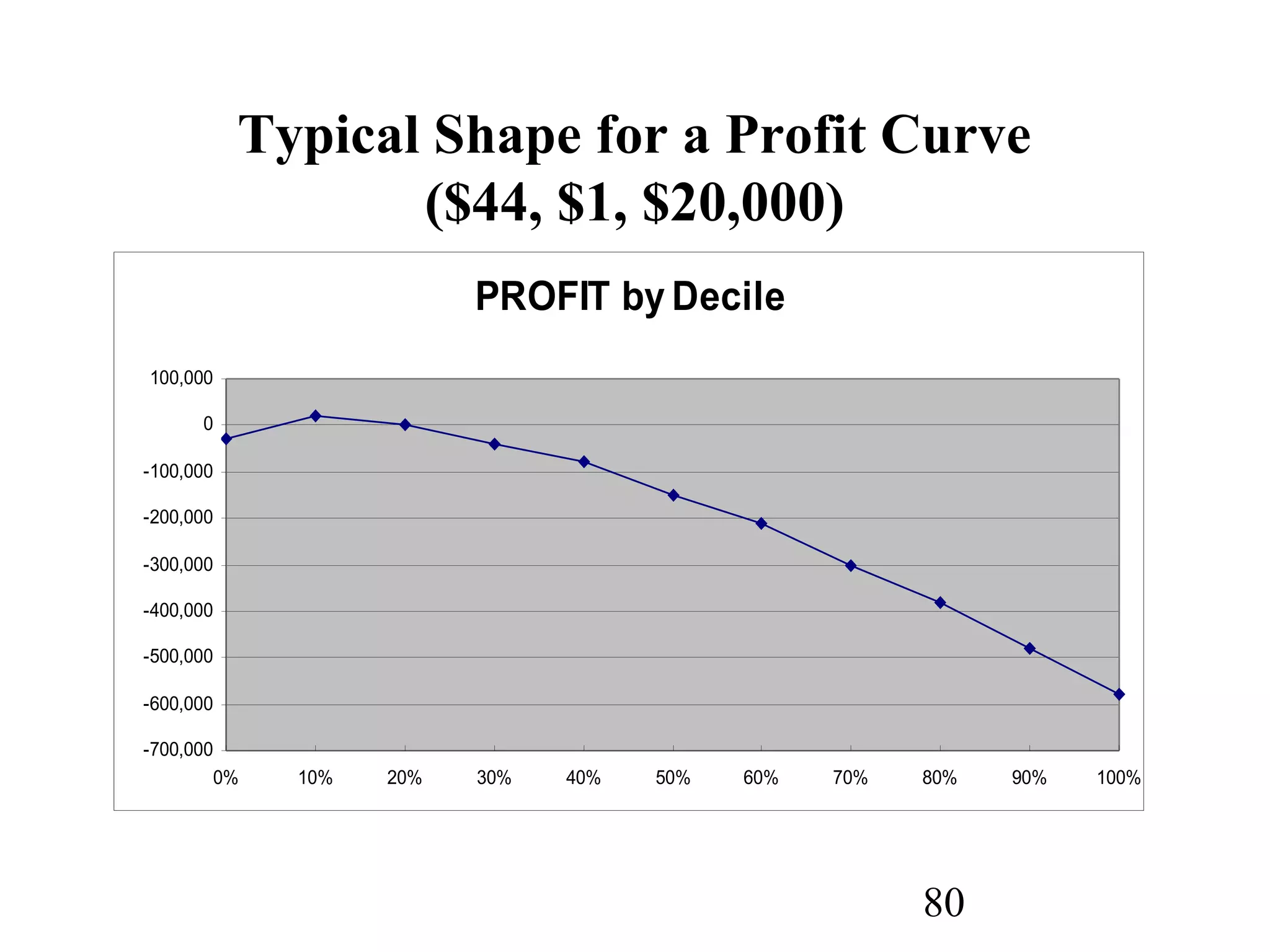
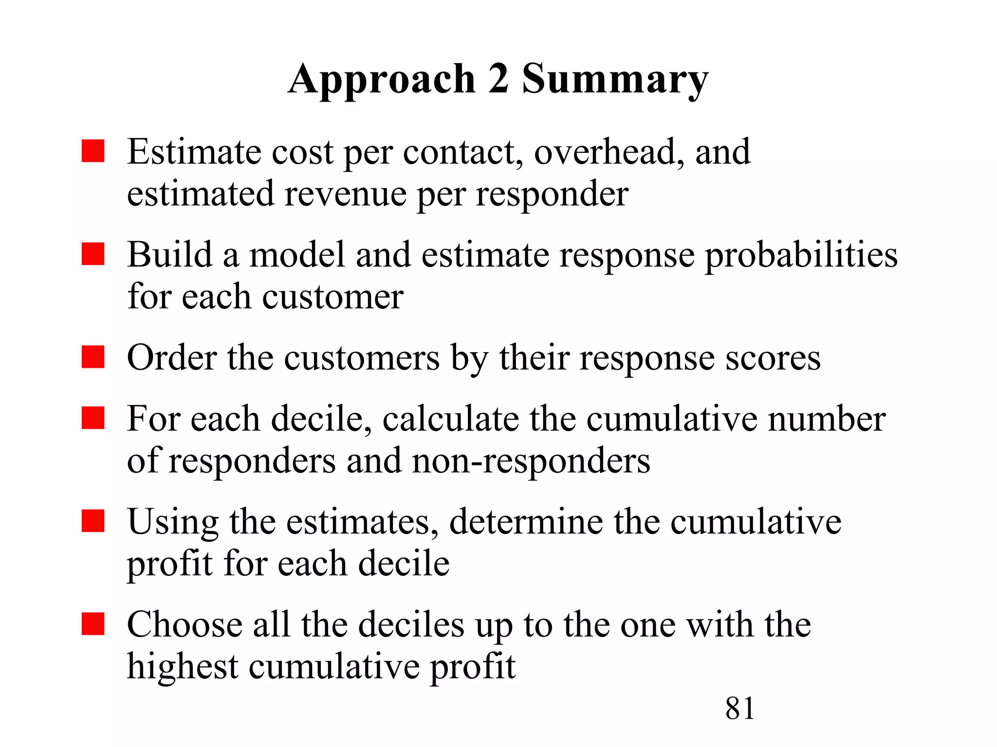
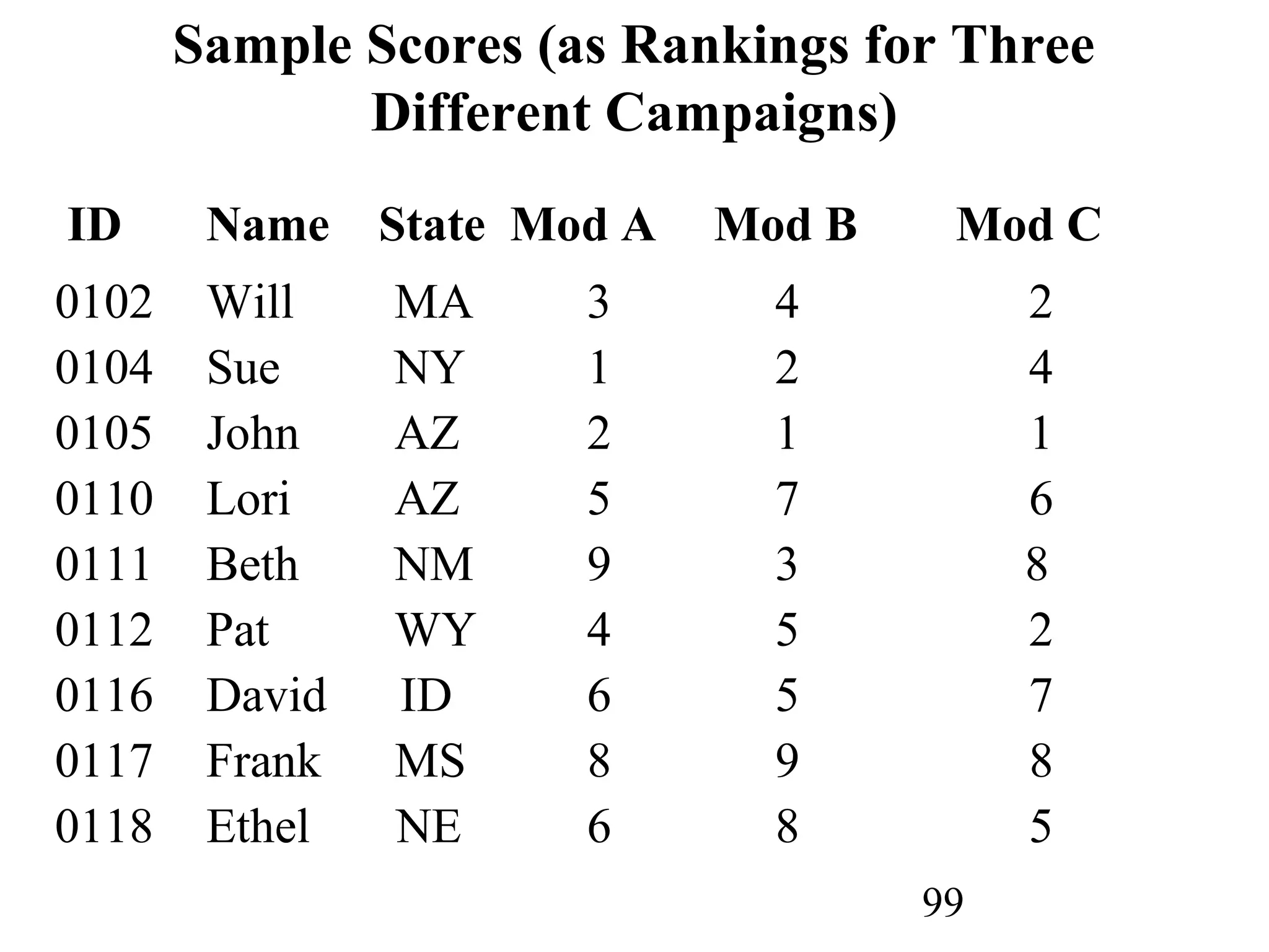
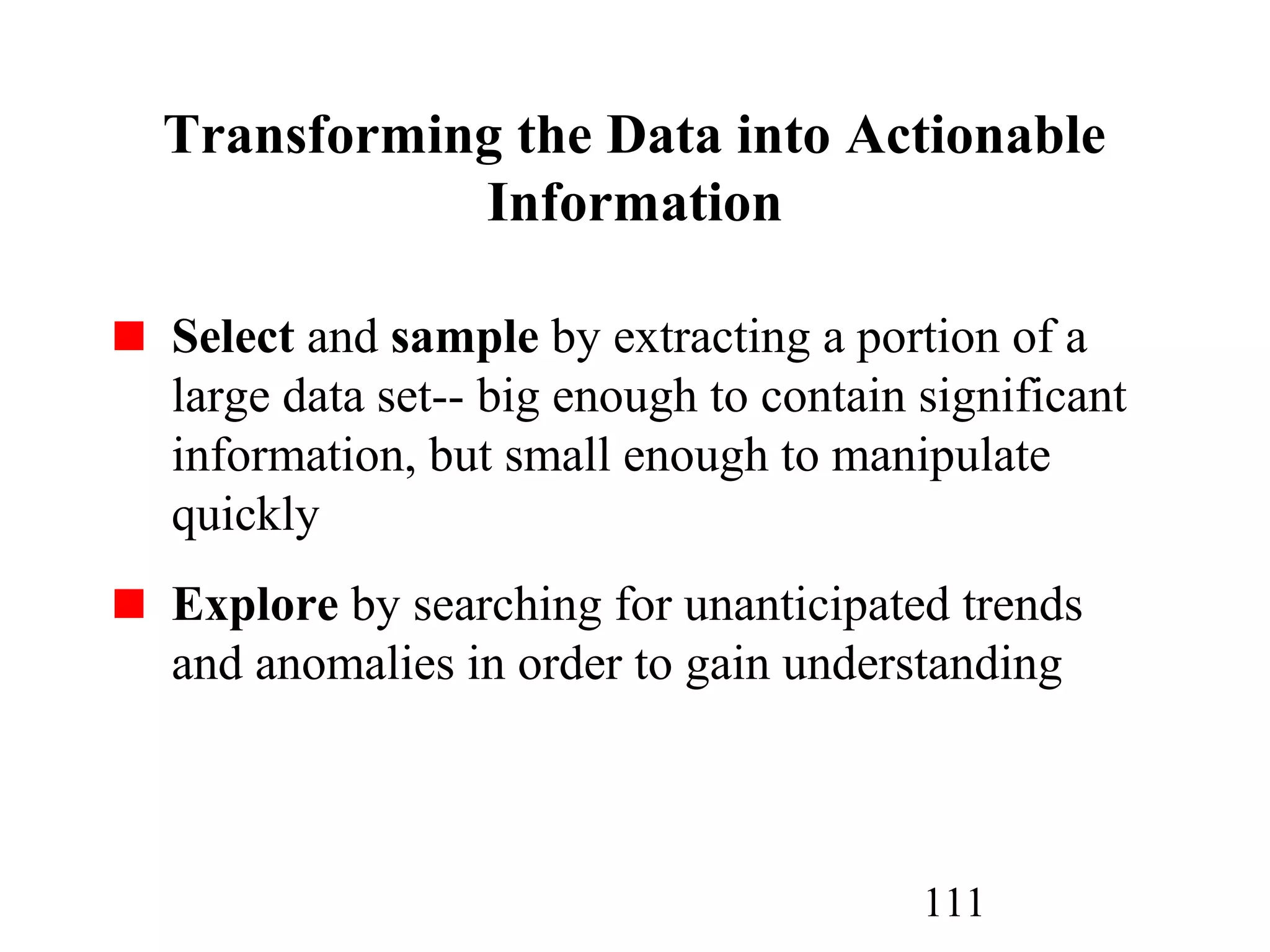
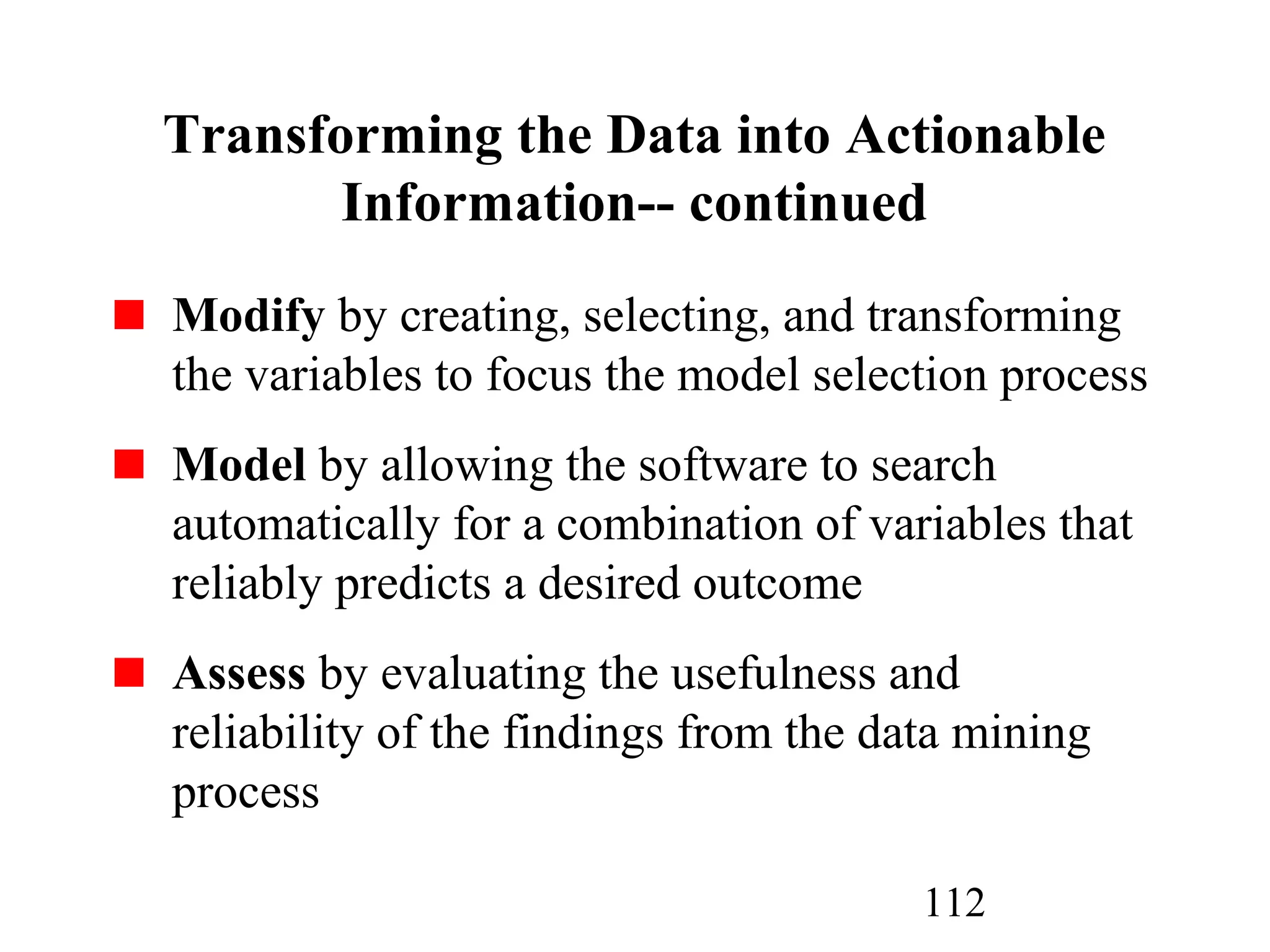
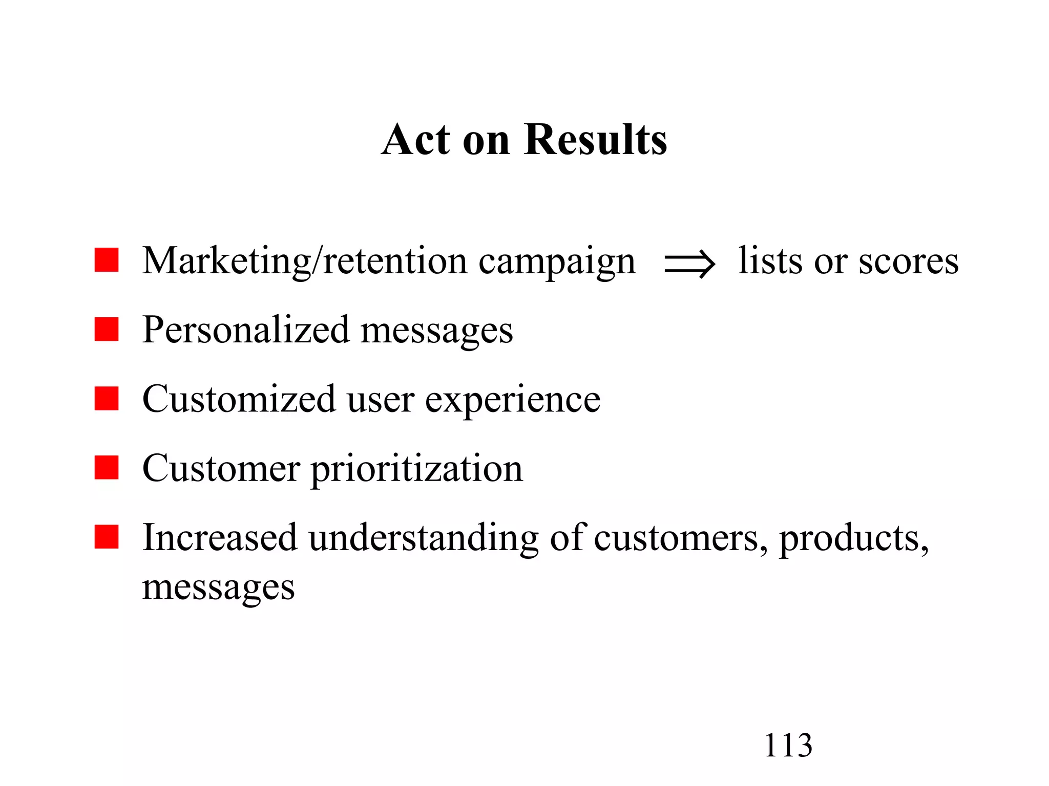
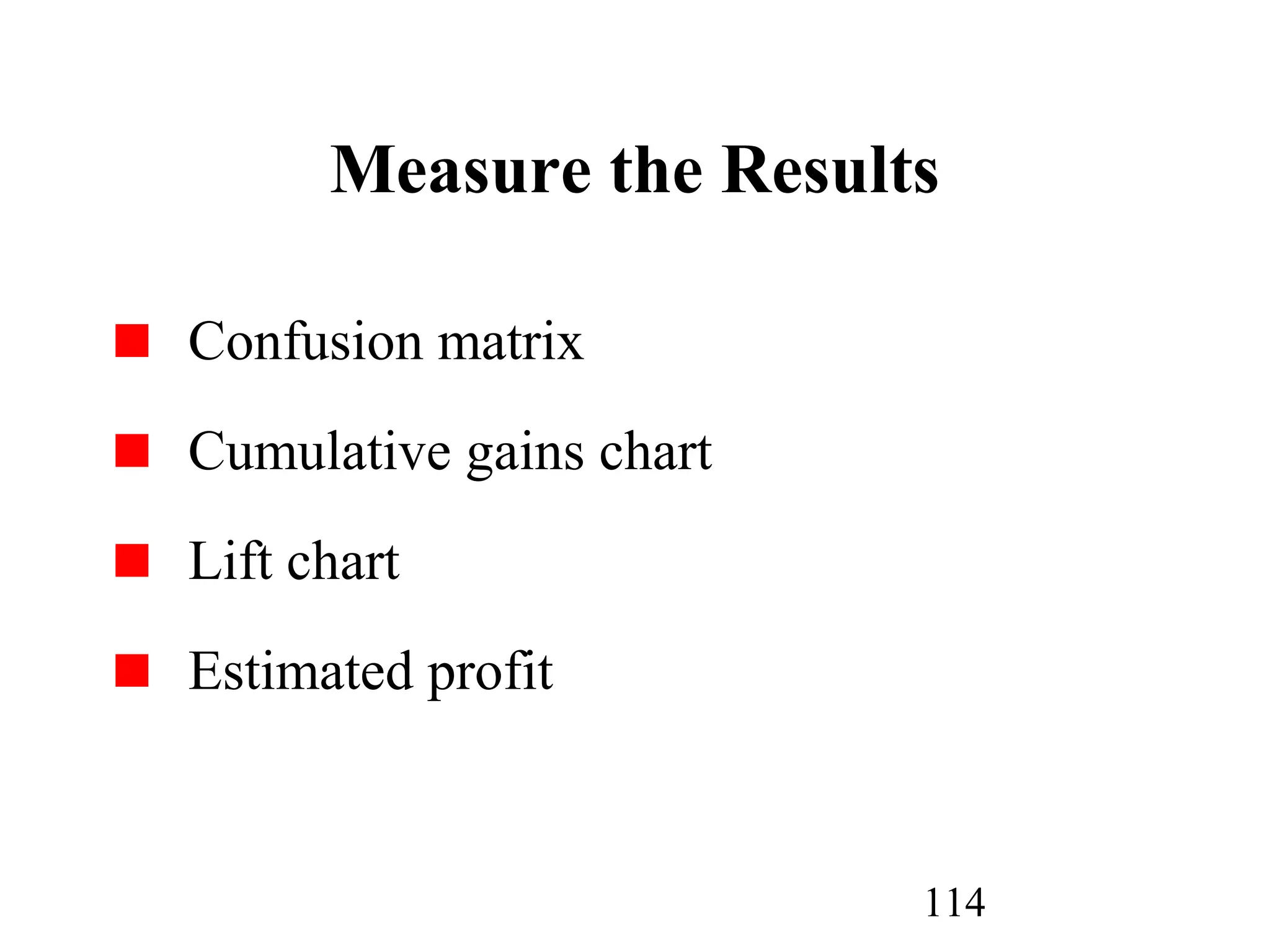
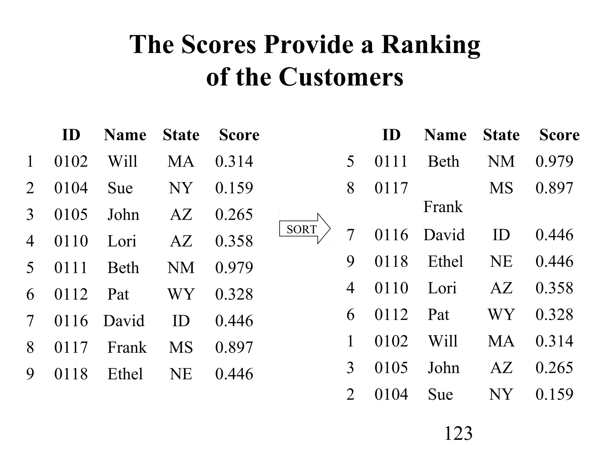
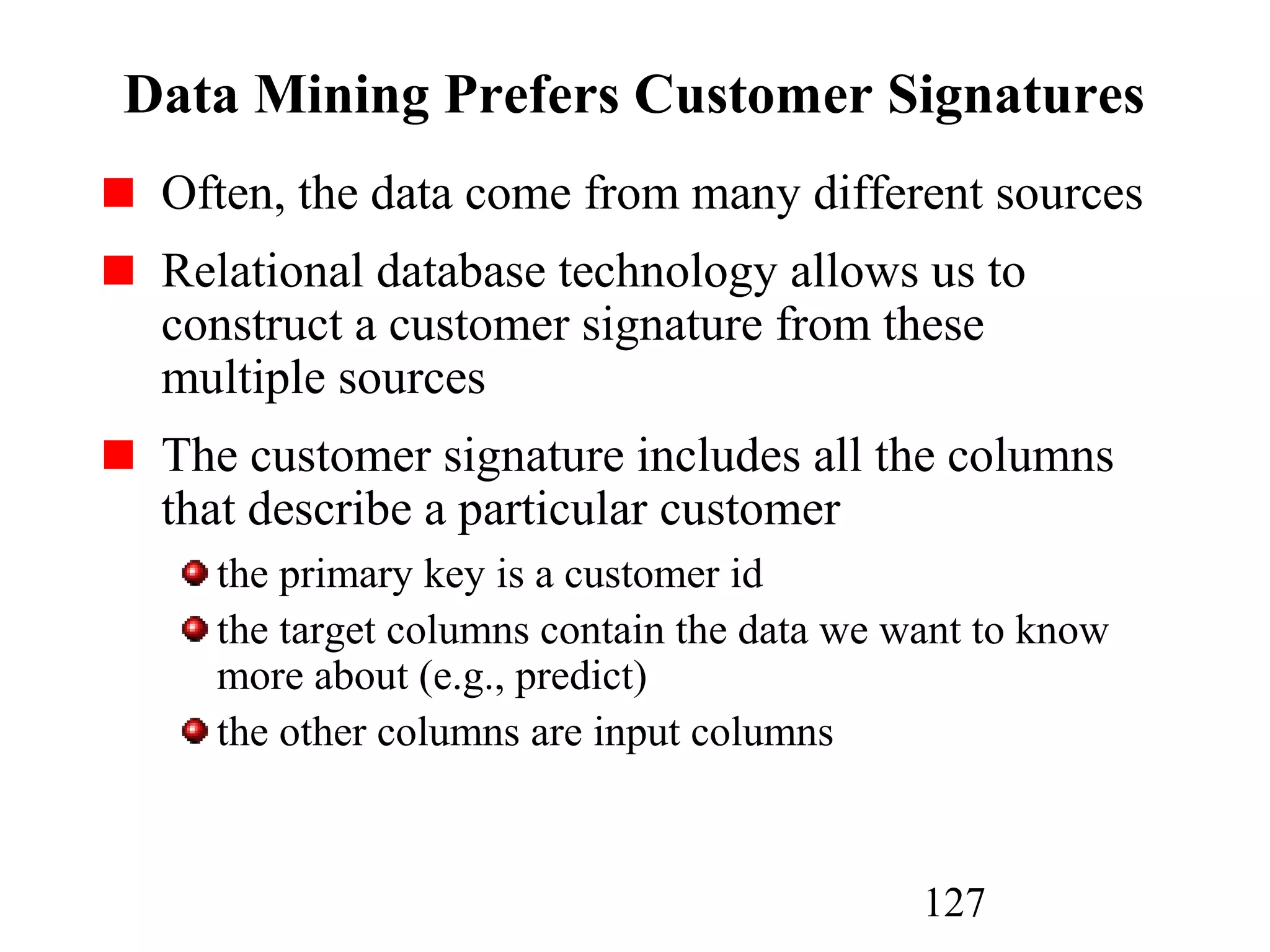
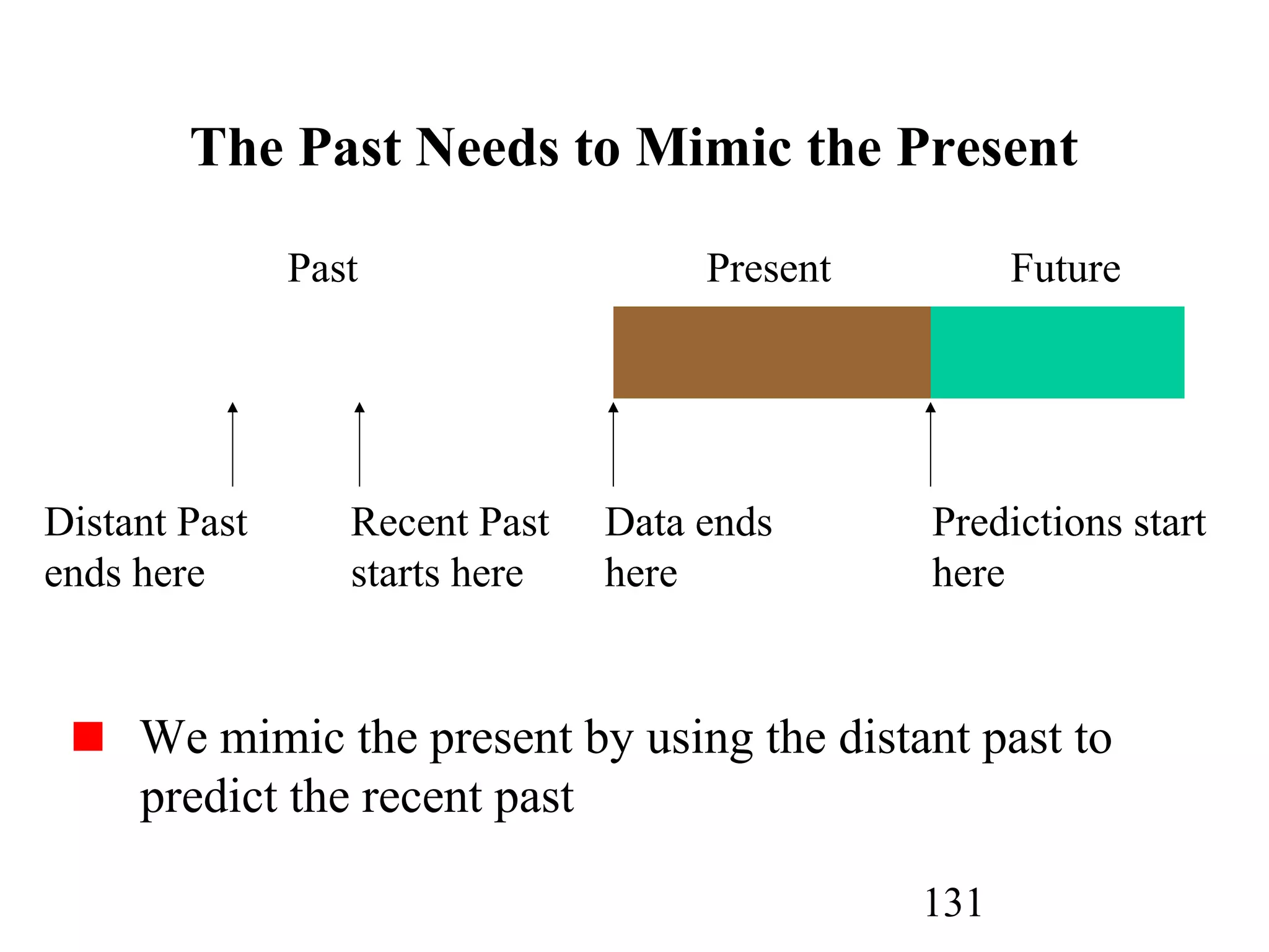
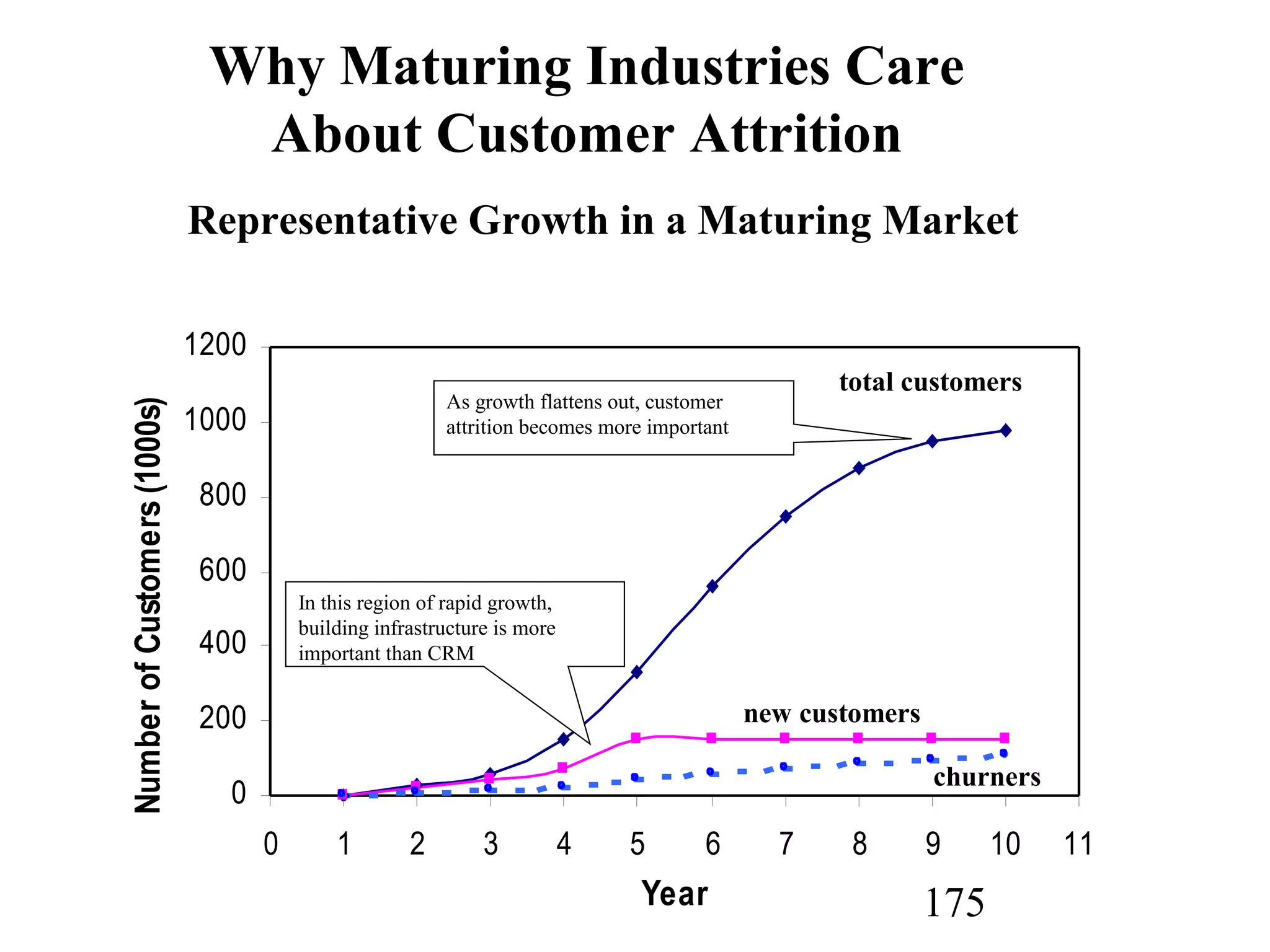
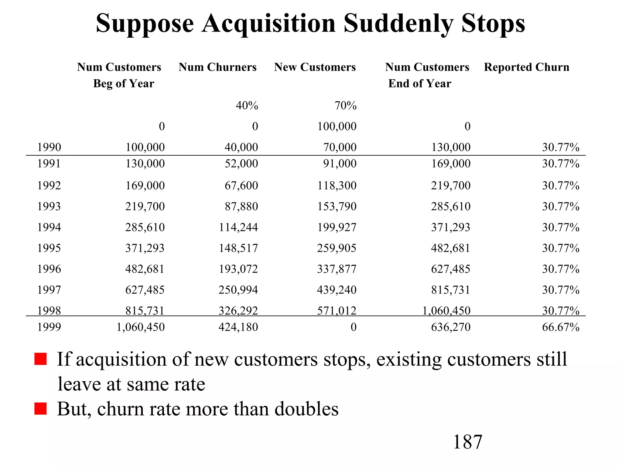
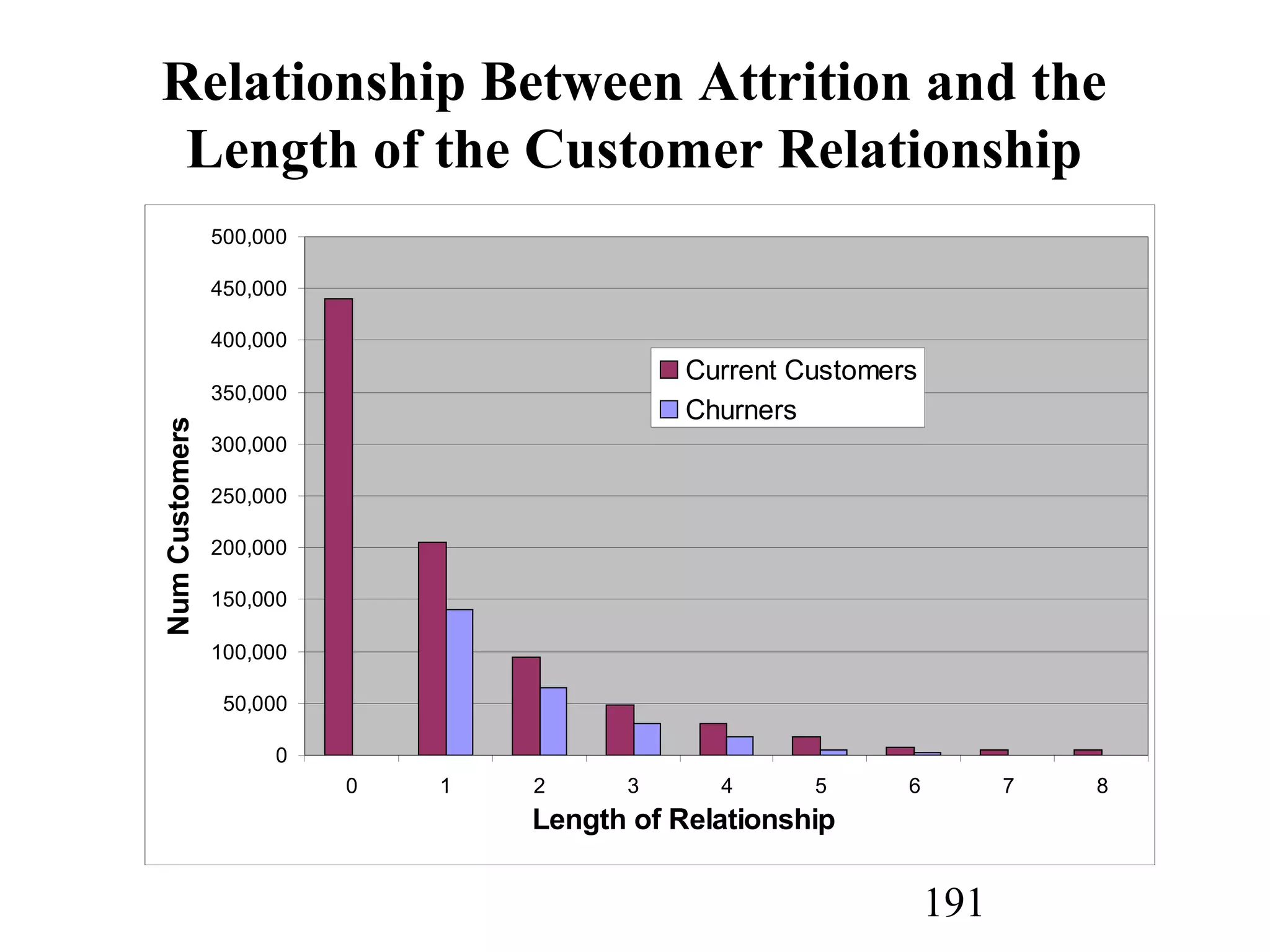
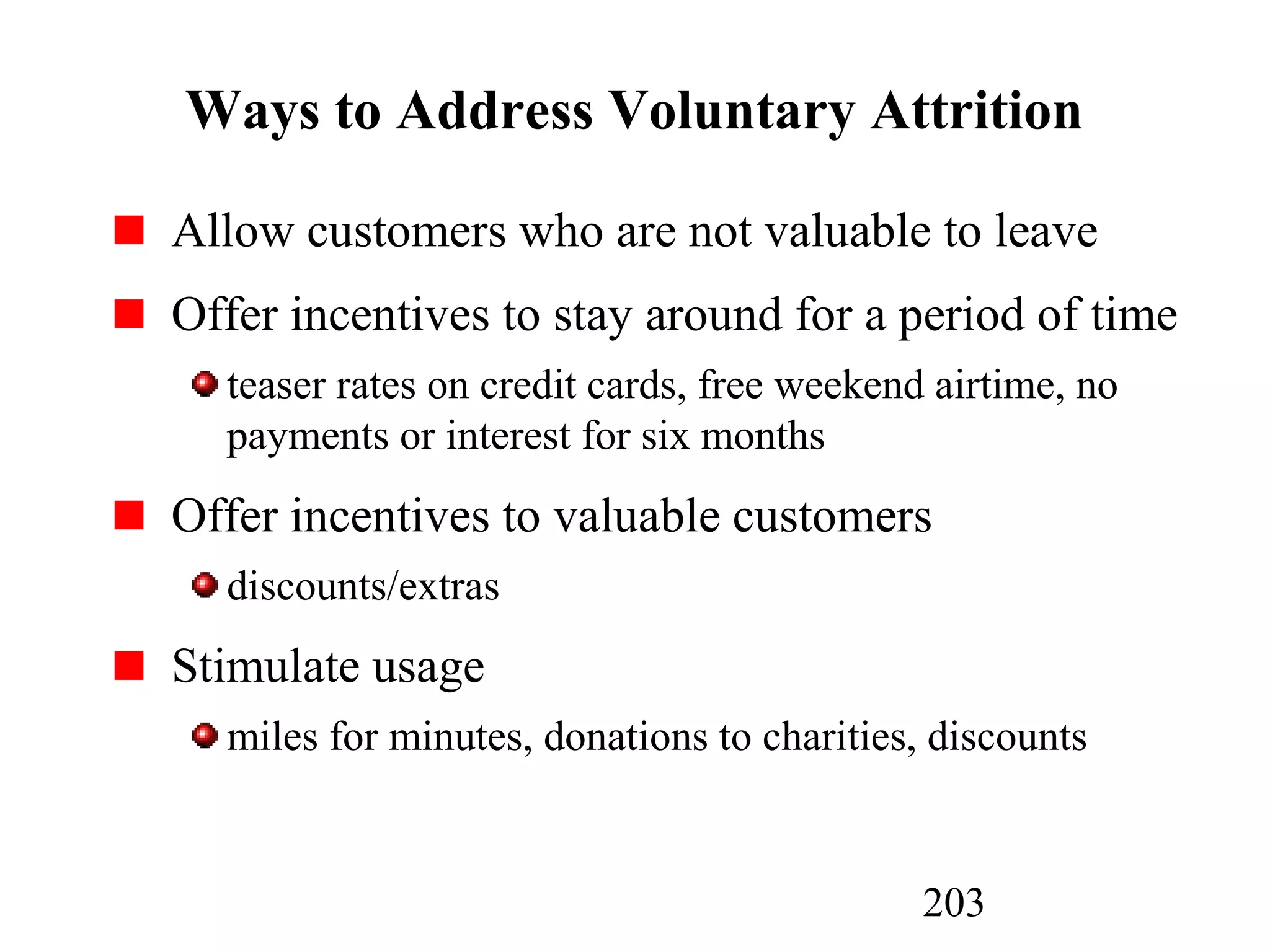
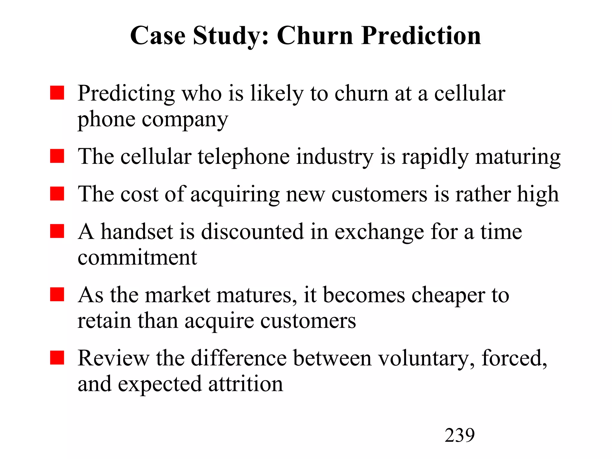
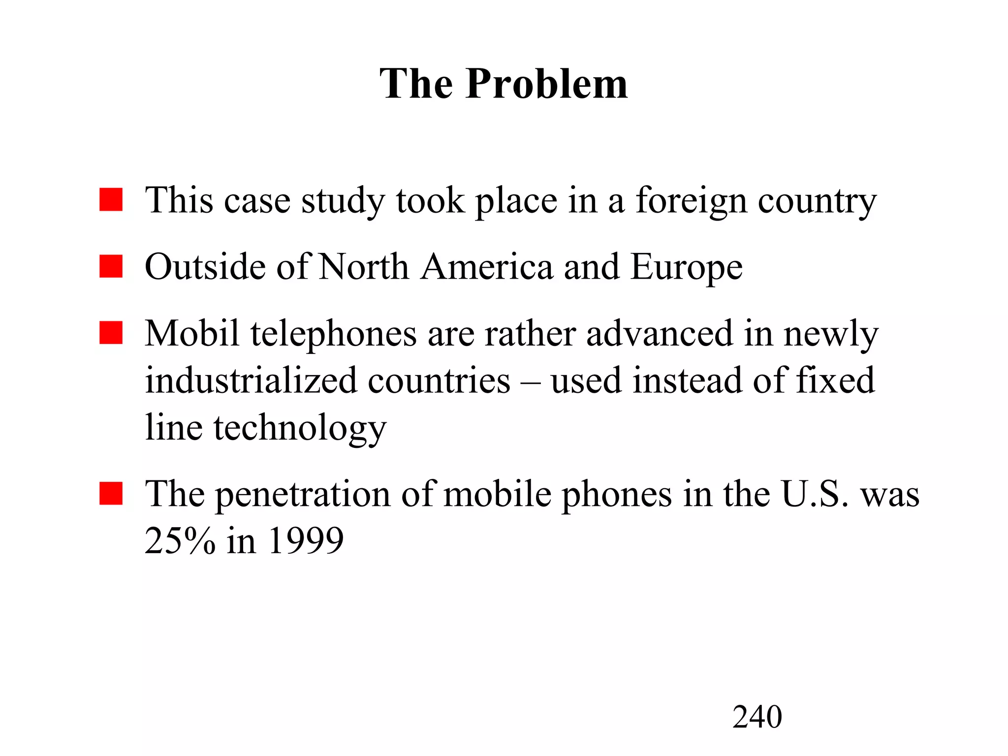
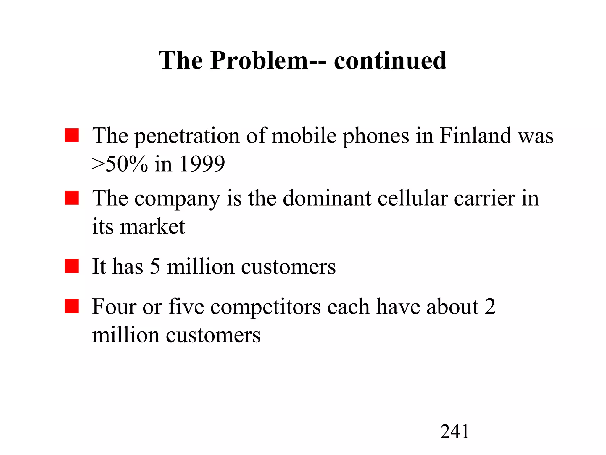
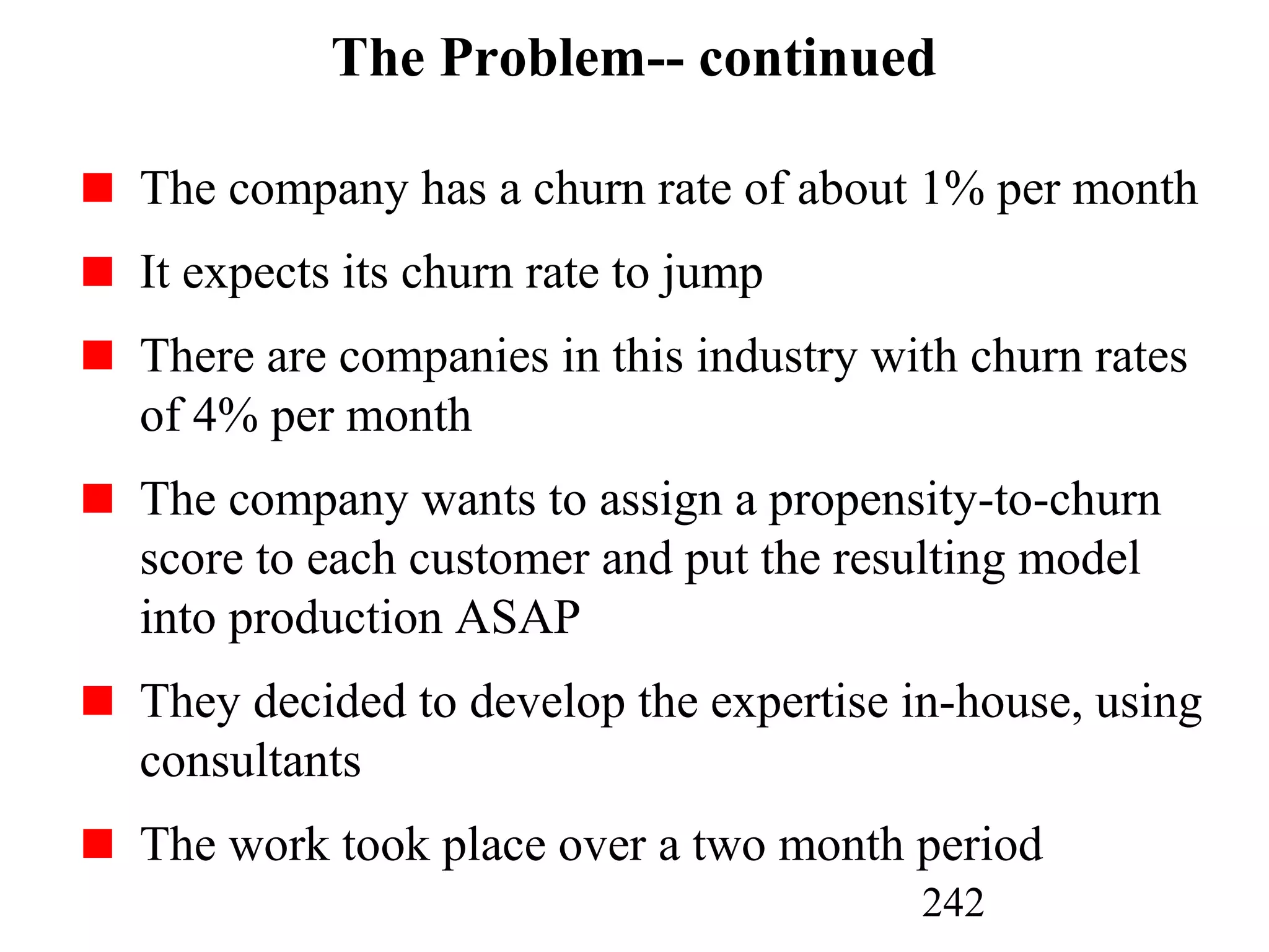
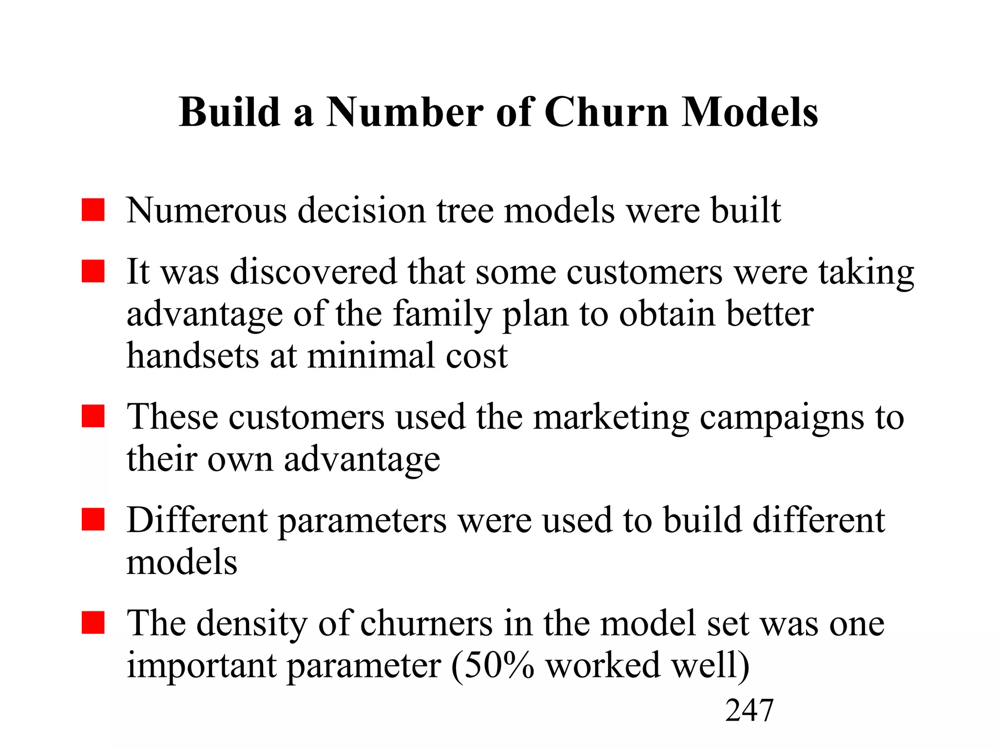
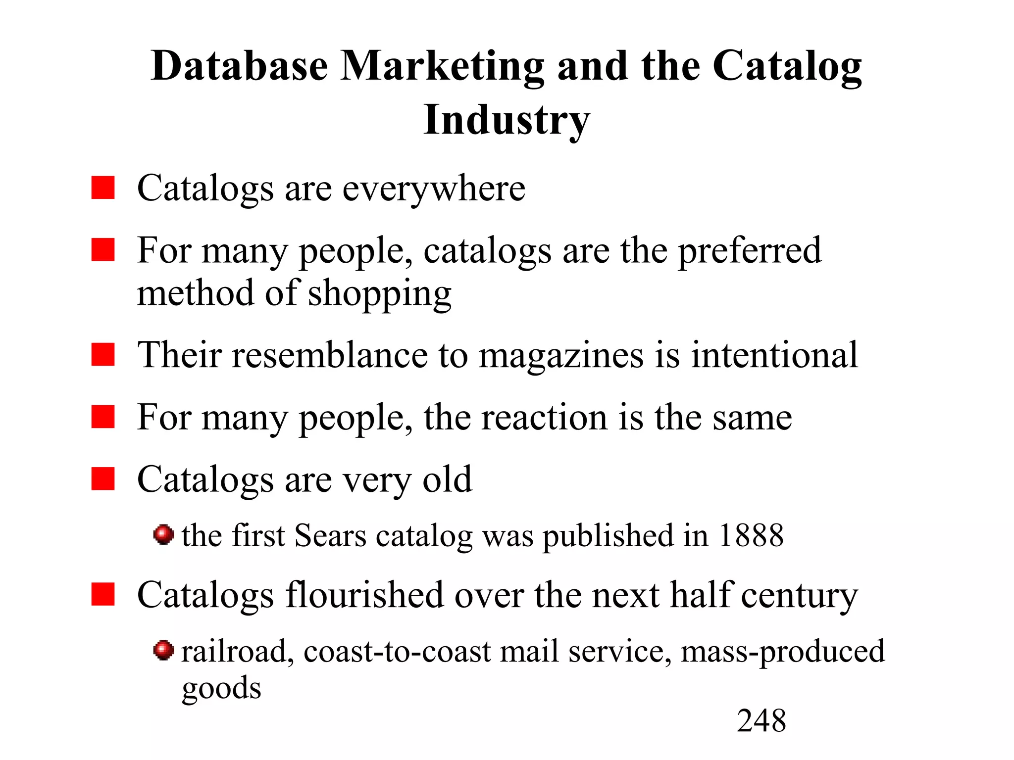
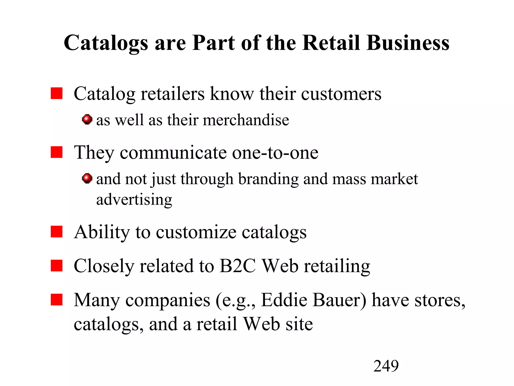
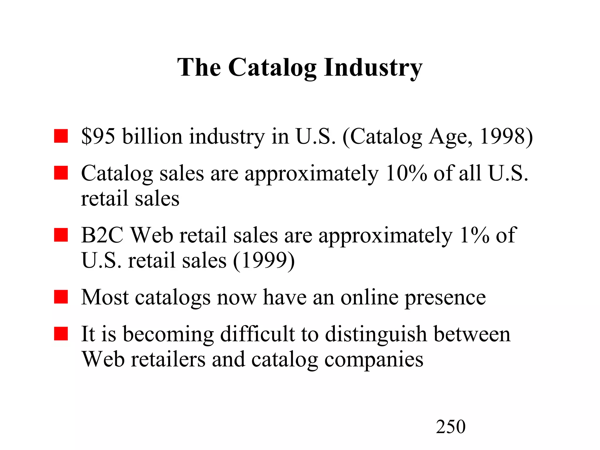
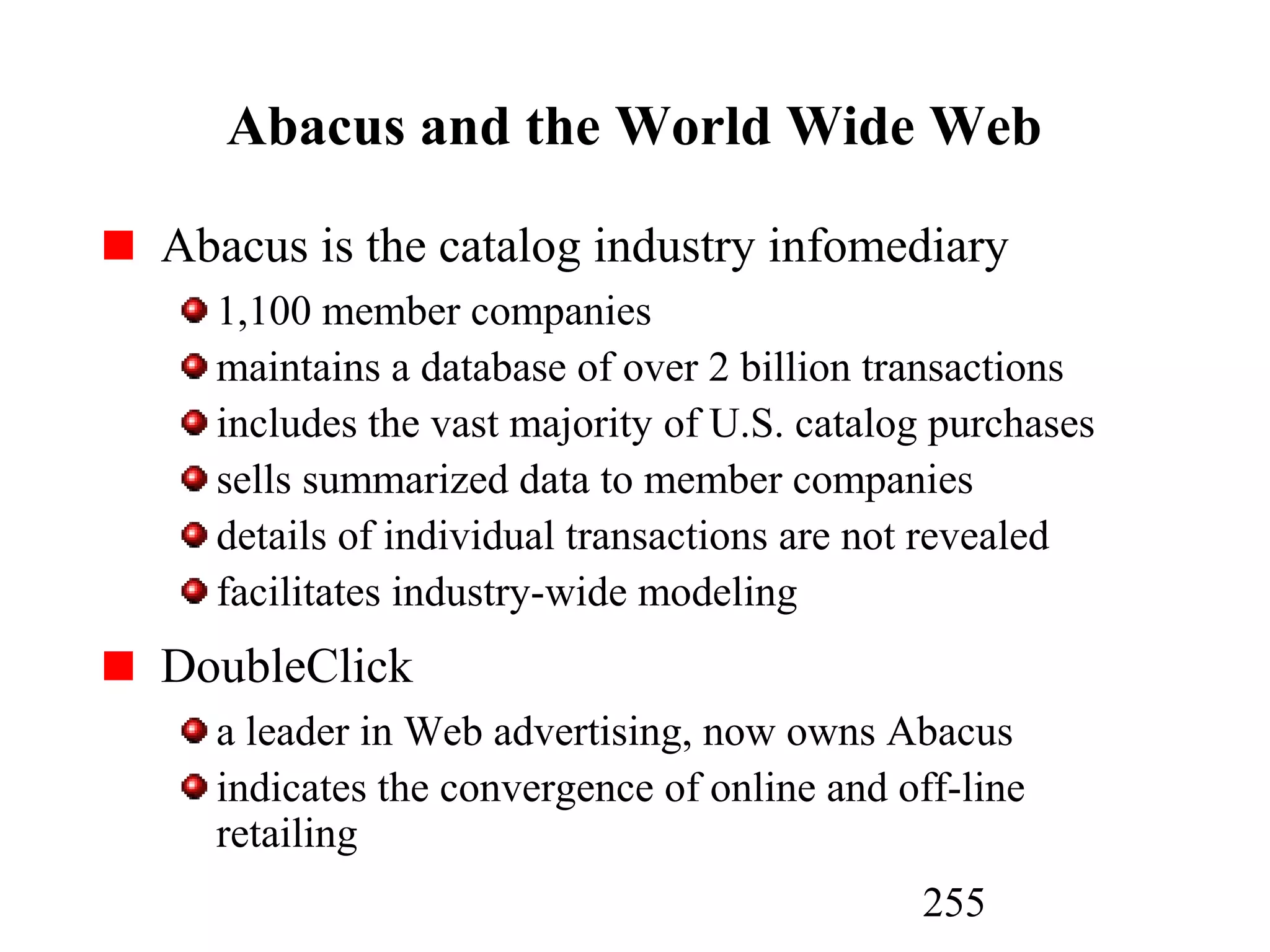
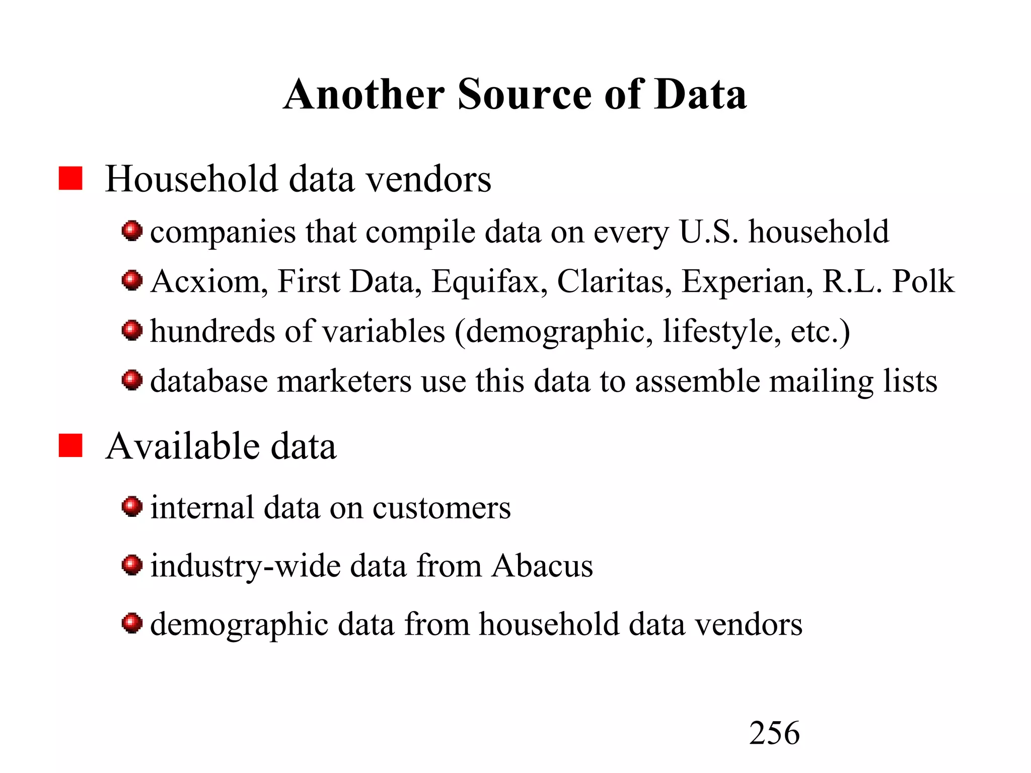
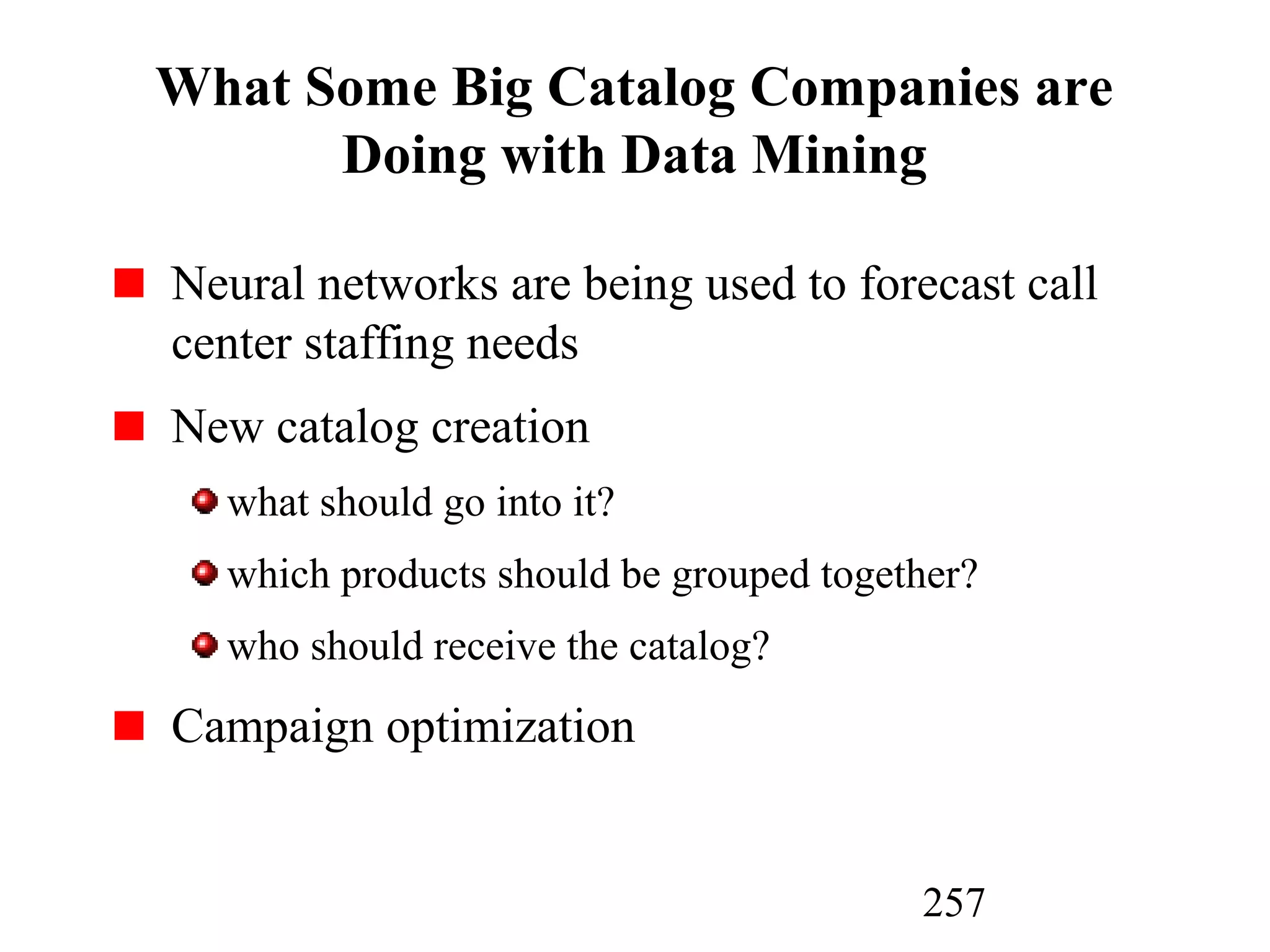
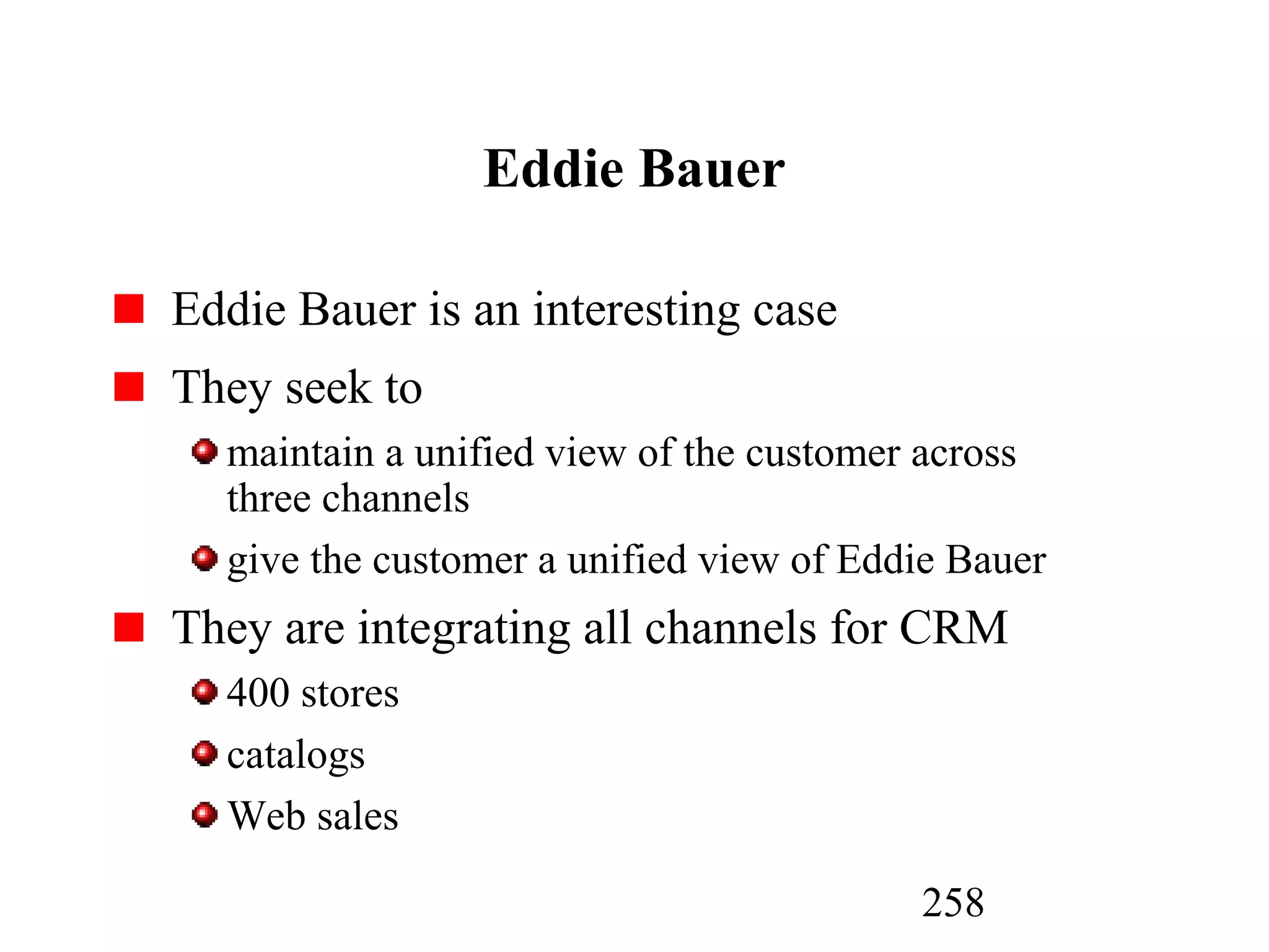
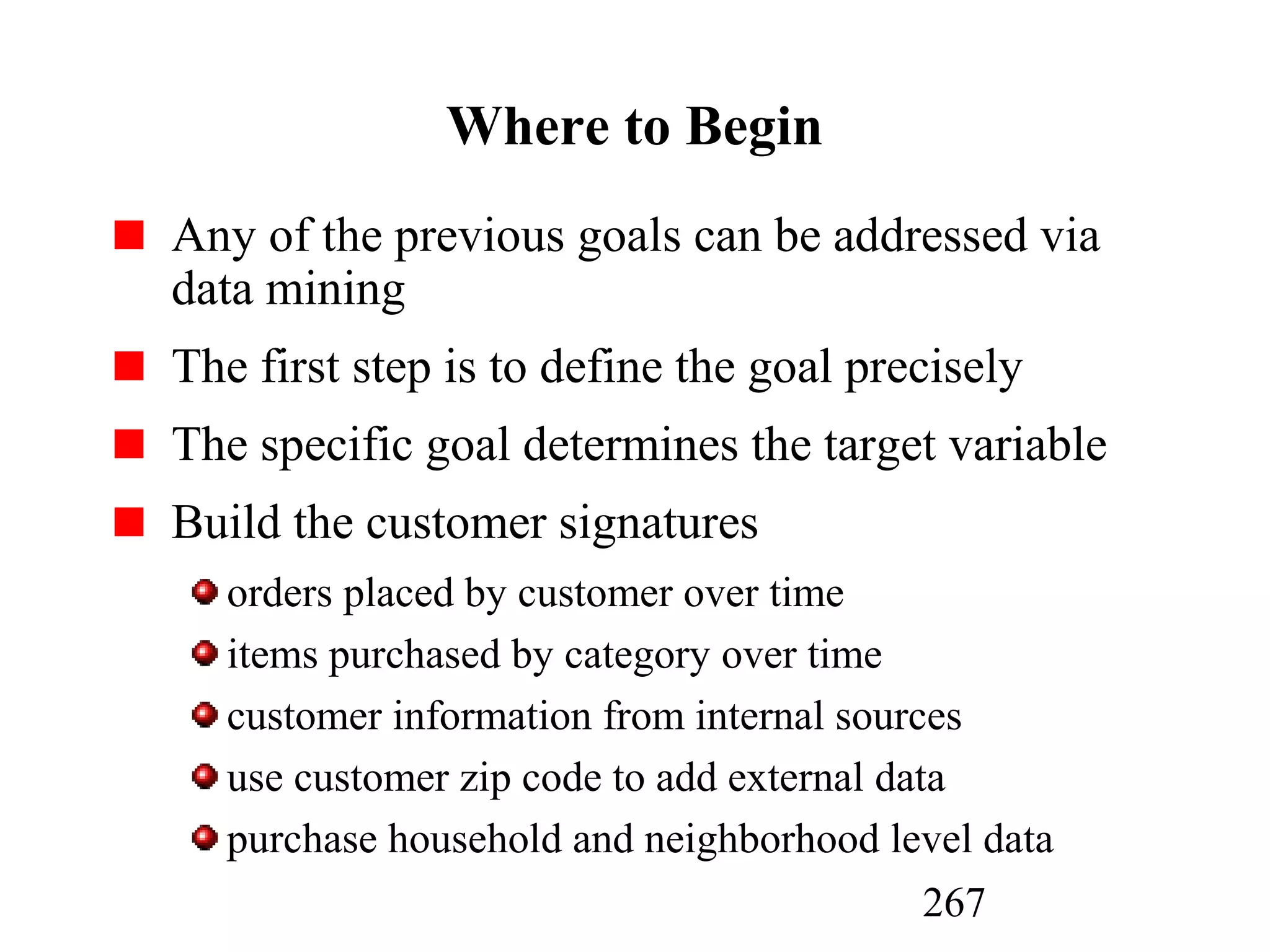
The document discusses customer relationship management (CRM) through data mining. It describes how CRM focuses on viewing customers as a company's primary asset and knowing customers across all business units and channels. CRM aims to learn from customer data generated through interactions over various channels to continuously improve the customer experience and identify opportunities. Data mining plays a key role in CRM by providing insights into customer behavior and needs to help companies better acquire, serve, and retain customers.

1. 1
BUDT 725: Models and Applications
in Operations Research
by
Bruce L. Golden
R.H. Smith School of Business
Volume 1- Customer Relationship Management Through Data Mining

2. 2
Customer Relationship Management
Through Data Mining
Introduction to Customer Relationship Management
(CRM)
Introduction to Data Mining
Data Mining Software
Churn Modeling
Acquisition and Cross Sell Modeling

3. 3
Relationship Marketing
Relationship Marketing is a Process
communicating with your customers
listening to their responses
Companies take actions
marketing campaigns
new products
new channels
new packaging

4. 4
Relationship Marketing -- continued
Customers and prospects respond
most common response is no response
This results in a cycle
data is generated
opportunities to learn from the data and improve the
process emerge

5. 5
The Move Towards Relationship
Management
E-commerce companies want to customize the user
experience
Supermarkets want to be infomediaries
Credit card companies want to recommend good
restaurants and hotels in new cities
Phone companies want to know your friends and family
Bottom line: Companies want to be in the business of
serving customers rather than merely selling products

6. 6
CRM is Revolutionary
Grocery stores have been in the business of stocking
shelves
Banks have been in the business of managing the spread
between money borrowed and money lent
Insurance companies have been in the business of
managing loss ratios
Telecoms have been in the business of completing
telephone calls
Key point: More companies are beginning to view
customers as their primary asset

7. 7
Why Now ?
0
200
400
600
800
1000
1200
0 1 2 3 4 5 6 7 8 9 10 11
Year
NumberofCustomers(1000s)
As growth flattens out, exploiting
existing customers becomes more
important
In this region of rapid growth,
building infrastructure is more
important than CRM
total customers
new customers
churners
Representative Growth in a Maturing Market

8. 8
The Electronic Trail
A customer places a catalog order over the
telephone
At the local telephone company
time of call, number dialed, long distance
company used, …
At the long distance company (for the toll-free
number)
duration of call, route through switching system, …
At the catalog
items ordered, call center, promotion response,
credit card used, inventory update, shipping method
requested, …

9. 9
The Electronic Trail-- continued
At the credit card clearing house
transaction date, amount charged, approval code,
vendor number, …
At the bank
billing record, interest rate, available credit
update, …
At the package carrier
zip code, time stamp at truck, time stamp at
sorting center, …
Bottom line: Companies do keep track of data

10. 10
An Illustration
A few years ago, UPS went on strike
FedEx saw its volume increase
After the strike, its volume fell
FedEx identified those customers whose FedEx
volumes had increased and then decreased
These customers were using UPS again
FedEx made special offers to these customers to
get all of their business

11. 11
The Corporate Memory
Several years ago, Land’s End could not
recognize regular Christmas shoppers
some people generally don’t shop from catalogs
but spend hundreds of dollars every Christmas
if you only store 6 months of history, you will miss
them
Victoria’s Secret builds customer loyalty with a
no-hassle returns policy
some “loyal customers” return several expensive
outfits each month
they are really “loyal renters”

12. 12
CRM Requires Learning and More
Form a learning relationship with your
customers
Notice their needs
On-line Transaction Processing Systems
Remember their preferences
Decision Support Data Warehouse
Learn how to serve them better
Data Mining
Act to make customers more profitable

13. 13
The Importance of Channels
Channels are the way a company interfaces with
its customers
Examples
Direct mail
Email
Banner ads
Telemarketing
Billing inserts
Customer service centers
Messages on receipts
Key data about customers come from channels

14. 14
Channels -- continued
Channels are the source of data
Channels are the interface to customers
Channels enable a company to get a particular
message to a particular customer
Channel management is a challenge in
organizations
CRM is about serving customers through all
channels

15. 15
Where Does Data Mining Fit In?
Hindsight
Foresight
Insight
Analysis and
Reporting (OLAP)
Statistical
Modeling
Data
Mining

16. 16
Our Definition of Data Mining
Exploration and analysis of large quantities of data
By automatic or semi-automatic means
To discover meaningful patterns and rules
These patterns allow a company to
better understand its customers
improve its marketing, sales, and customer support
operations
Source: Berry and Linoff (1997)

17. 17
Data Mining for Insight
Classification
Prediction
Estimation
Automatic Cluster Detection
Affinity Grouping
Description

18. 18
Finding Prospects
A cellular phone company wanted to
introduce a new service
They wanted to know which customers were
the most likely prospects
Data mining identified “sphere of influence”
as a key indicator of likely prospects
Sphere of influence is the number of
different telephone numbers that someone
calls

19. 19
Paying Claims
A major manufacturer of diesel engines must also
service engines under warranty
Warranty claims come in from all around the world
Data mining is used to determine rules for routing
claims
some are automatically approved
others require further research
Result: The manufacturer saves millions of dollars
Data mining also enables insurance companies and
the Fed. Government to save millions of dollars by
not paying fraudulent medical insurance claims

20. 20
Cross Selling
Cross selling is another major application of data
mining
What is the best additional or best next offer
(BNO) to make to each customer?
E.g., a bank wants to be able to sell you
automobile insurance when you get a car loan
The bank may decide to acquire a full-service
insurance agency

21. 21
Holding on to Good Customers
Berry and Linoff used data mining to help a
major cellular company figure out who is at risk
for attrition
And why are they at risk
They built predictive models to generate call
lists for telemarketing
The result was a better focused, more effective
retention campaign

22. 22
Weeding out Bad Customers
Default and personal bankruptcy cost lenders
millions of dollars
Figuring out who are your worst customers can
be just as important as figuring out who are your
best customers
many businesses lose money on most of their
customers

23. 23
They Sometimes get Their Man
The FBI handles numerous, complex cases such
as the Unabomber case
Leads come in from all over the country
The FBI and other law enforcement agencies sift
through thousands of reports from field agents
looking for some connection
Data mining plays a key role in FBI forensics

24. 24
Clustering is an undirected data mining technique
that finds groups of similar items
Based on previous purchase patterns, customers are
placed into groups
Customers in each group are
assumed to have an affinity
for the same types of products
New product recommendations
can be generated automatically
based on new purchases made
by the group
This is sometimes called collaborative filtering
Anticipating Customer Needs

25. 25
CRM Focuses on the Customer
The enterprise has a unified view of each customer
across all business units and across all channels
This is a major systems integration task
The customer has a unified view of the enterprise
for all products and regardless of channel
This requires harmonizing all the channels

26. 26
A Continuum of Customer Relationships
Large accounts have sales managers and
account teams
E.g., Coca-Cola, Disney, and McDonalds
CRM tends to focus on the smaller customer
--the consumer
But, small businesses are also good candidates
for CRM

27. 27
What is a Customer
A transaction?
An account?
An individual?
A household?
The customer as a transaction
purchases made with cash are anonymous
most Web surfing is anonymous
we, therefore, know little about the consumer

28. 28
A Customer is an Account
More often, a customer is an account
Retail banking
checking account, mortgage, auto loan, …
Telecommunications
long distance, local, ISP, mobile, …
Insurance
auto policy, homeowners, life insurance, …
Utilities
The account-level view of a customer also
misses the boat since each customer can have
multiple accounts

29. 29
Customers Play Different Roles
Parents buy back-to-school clothes for teenage
children
children decide what to purchase
parents pay for the clothes
parents “own” the transaction
Parents give college-age children cellular phones or
credit cards
parents may make the purchase decision
children use the product
It is not always easy to identify the customer

30. 30
The Customer’s Lifecycle
Childhood
birth, school, graduation, …
Young Adulthood
choose career, move away from parents, …
Family Life
marriage, buy house, children, divorce, …
Retirement
sell home, travel, hobbies, …
Much marketing effort is directed at each stage
of life

31. 31
The Customer’s Lifecycle is Unpredictable
It is difficult to identify the appropriate events
graduation, retirement may be easy
marriage, parenthood are not so easy
many events are “one-time”
Companies miss or lose track of valuable
information
a man moves
a woman gets married, changes her last name, and
merges her accounts with spouse
It is hard to track your customers so closely, but,
to the extent that you can, many marketing
opportunities arise

32. 32
Customers Evolve Over Time
Customers begin as prospects
Prospects indicate interest
fill out credit card applications
apply for insurance
visit your website
They become new customers
After repeated purchases or usage, they become
established customers
Eventually, they become former customers
either voluntarily or involuntarily

33. 33
Business Processes Organize Around the
Customer Lifecycle
Acquisition Activation Relationship Management Winback
Former
Customer
Prospect Established
Customer
New
Customer
Low
Value
High
Potential
High
Value
Voluntary
Churn
Forced
Churn

34. 34
Different Events Occur
Throughout the Lifecycle
Prospects receive marketing messages
When they respond, they become new customers
They make initial purchases
They become established customers and are
targeted by cross-sell and up-sell campaigns
Some customers are forced to leave (cancel)
Some leave (cancel) voluntarily
Others simply stop using the product (e.g., credit
card)
Winback/collection campaigns

35. 35
Different Data is Available
Throughout the Lifecycle
The purpose of data warehousing is to keep this
data around for decision-support purposes
Charles Schwab wants to handle all of their
customers’ investment dollars
Schwab observed that customers started with
small investments

36. 36
Different Data is Available
Throughout the Lifecycle -- continued
By reviewing the history of many customers,
Schwab discovered that customers who
transferred large amounts into their Schwab
accounts did so soon after joining
After a few months, the marketing cost could not
be justified
Schwab’s marketing strategy changed as a result

37. 37
Different Models are Appropriate
at Different Stages
Prospect acquisition
Prospect product propensity
Best next offer
Forced churn
Voluntary churn
Bottom line: We use data mining to predict
certain events during the customer lifecycle

38. 38
Different Approaches to Data Mining
Outsourcing
let an outside expert do the work
have him/her report the results
Off-the-shelf, turn-key software solutions
packages have generic churn models &
response models
they work pretty well
Master Data Mining
develop expertise in-house
use sophisticated software such as
Clementine or Enterprise Miner

39. 39
Privacy is a Serious Matter
Data mining and CRM raise some privacy
concerns
These concerns relate to the collection of data,
more than the analysis of data
The next few slides illustrate marketing mistakes
that can result from the abundance and availability
of data

40. 40
Using Data Mining to Help Diabetics
Early detection of diabetes can save money by
preventing more serious complications
Early detection of complications can prevent
worsening
retinal eye exams every 6 or 12 months can prevent
blindness
these eye exams are relatively inexpensive
So one HMO took action
they decided to encourage their members, who had
diabetes to get eye exams
the IT group was asked for a list of members with
diabetes

41. 41
One Woman’s Response
Letters were sent out to HMO members
Three types of diabetes – congenital, adult-onset,
gestational
One woman contacted had gestational diabetes
several years earlier
She was “traumatized” by the letter, thinking the
diabetes had recurred
She threatened to sue the HMO
Mistake: Disconnect between the domain
expertise and data expertise

42. 42
Gays in the Military
The “don’t ask; don’t tell” policy allows
discrimination against openly gay men and
lesbians in the military
Identification as gay or lesbian is sufficient
grounds for discharge
This policy is enforced
Approximately 1000 involuntary discharges each
year

43. 43
The Story of Former Senior Chief
Petty Officer Timothy McVeigh
Several years ago, McVeigh used an AOL account,
with an anonymous alias
Under marital status, he listed “gay”
A colleague discovered the account and called AOL
to verify that the owner was McVeigh
AOL gave out the information over the phone
McVeigh was discharged (three years short of his
pension)
The story doesn’t end here

44. 44
Two Serious Privacy Violations
AOL breached its own policy by giving out
confidential user information
AOL paid an undisclosed sum to settle with McVeigh
and suffered bad press as well
The law requires that government agents identify
themselves to get online subscription information
This was not done
McVeigh received an honorable discharge with full
retirement pension

45. 45
Friends, Family, and Others
In the 1990s, MCI promoted the “Friends and
Family” program
They asked existing customers for names of
people they talked with often
If these friends and family signed up with MCI,
then calls to them would be discounted
Did MCI have to ask customers about who they
call regularly?
Early in 1999, BT (formerly British Telecom)
took the idea one step beyond
BT invented a new marketing program
discounts to the most frequently called numbers

46. 46
BT Marketing Program
BT notified prospective customers of this
program by sending them their most frequently
called numbers
One woman received the letter
uncovered her husband’s cheating
threw him out of the house
sued for divorce
The husband threatened to sue BT for violating
his privacy
BT suffered negative publicity

47. 47
No Substitute for Human Intelligence
Data mining is a tool to achieve goals
The goal is better service to customers
Only people know what to predict
Only people can make sense of rules
Only people can make sense of visualizations
Only people know what is reasonable, legal,
tasteful
Human decision makers are critical to the data
mining process

48. 48
A Long, Long Time Ago
There was no marketing
There were few manufactured goods
Distribution systems were slow and uncertain
There was no credit
Most people made what they needed at home
There were no cell phones
There was no data mining
It was sufficient to build a quality product and
get it to market

49. 49
Then and Now
Before supermarkets, a typical grocery store
carried 800 different items
A typical grocery store today carries tens of
thousands of different items
There is intense competition for shelf space and
premium shelf space
In general, there has been an explosion in the
number of products in the last 50 years
Now, we need to anticipate and create demand
(e.g., e-commerce)
This is what marketing is all about

50. 50
Effective Marketing Presupposes
High quality goods and services
Effective distribution of goods and services
Adequate customer service
Marketing promises are kept
Competition
direct (same product)
“wallet-share”
Ability to interact directly with customers

51. 51
The ACME Corporation
Imagine a fictitious corporation that builds widgets
It can sell directly to customers via a catalog or the
Web
maintain control over brand and image
It can sell directly through retail channels
get help with marketing and advertising
It can sell through resellers
outsource marketing and advertising entirely
Let’s assume ACME takes the direct marketing
approach

52. 52
Before Focusing on One-to-One
Marketing
Branding is very important
provides a mark of quality to consumers
old concept – Bordeaux wines, Chinese porcelain,
Bruges cloth
really took off in the 20th
Century
Advertising is hard
media mix problem – print, radio, TV, billboard, Web
difficult to measure effectiveness
“Half of my advertising budget is wasted; I just don’t
know which half.”

53. 53
Different Approaches to Direct Marketing
Naïve Approach
get a list of potential customers
send out a large number of messages and repeat
Wave Approach
send out a large number of messages and test
Staged Approach
send a series of messages over time
Controlled Approach
send out messages over time to control response (e.g.,
get 10,000 responses/week)

54. 54
The World is Speeding Up
Advertising campaigns take months
market research
design and print material
Catalogs are planned seasons in advance
Direct mail campaigns also take months
Telemarketing campaigns take weeks
Web campaigns take days
modification/refocusing is easy

55. 55
How Data Mining Helps in
Marketing Campaigns
Improves profit by limiting campaign to most
likely responders
Reduces costs by excluding individuals least
likely to respond
AARP mails an invitation to those who turn 50
they excluded the bottom 10% of their list
response rate did not suffer

56. 56
How Data Mining Helps in
Marketing Campaigns--continued
Predicts response rates to help staff call centers,
with inventory control, etc.
Identifies most important channel for each
customer
Discovers patterns in customer data

57. 57
Some Background on ACME
They are going to pursue a direct marketing
approach
Direct mail marketing budget is $300,000
Best estimates indicate between 1 and 10 million
customers
ACME wants to target the customer base cost-
effectively
ACME seeks to assign a “score” to each customer
which reflects the relative likelihood of that
customer purchasing the product

58. 58
How Do You Assign Scores
Randomly – everyone gets the same score
Assign relative scores based on ad-hoc business
knowledge
Assign a score to each cell in an RFM (recency,
frequency, monetary) analysis
Profile existing customers and use these profiles
to assign scores to similar, potential customers
Build a predictive model based on similar product
sales in the past

59. 59
ID Name State Score Rank
0102 Will MA 0.314 7
0104 Sue NY 0.159 9
0105 John AZ 0.265 8
0110 Lori AZ 0.358 5
0111 Beth NM 0.979 1
0112 Pat WY 0.328 6
0116 David ID 0.446 4
0117 Frank MS 0.897 2
0118 Ethel NE 0.446 4
Data Mining Models Assign a Score
to Each Customer
Comments
1. Think of score as
likelihood of
responding
2. Some scores
may be the same

60. 60
Approach 1: Budget Optimization
ACME has a budget of $300,000 for a direct mail
campaign
Assumptions
each item being mailed costs $1
this cost assumes a minimum order of 20,000
ACME can afford to contact 300,000 customers
ACME contacts the highest scoring 300,000
customers
Let’s assume ACME is selecting from the top
three deciles

61. 61
The Concept of Lift
If we look at a random 10% of the potential
customers, we expect to get 10% of likely
responders
Can we select 10% of the potential customers and
get more than 10% of likely responders?
If so, we realize “lift”
This is a key goal in data mining

62. 62
Notes
1. x-axis gives
population
percentile
2. y-axis gives %
captured
responses
3. customers with
top 10% of the
scores account
for 30% of
responders
The Cumulative Gains Chart
0%
10%
20%
30%
40%
50%
60%
70%
80%
90%
100%
0% 10% 20% 30% 40% 50% 60% 70% 80% 90% 100%
ResponseModel
No Model

63. 63
Notes
1. x-axis gives
population
percentile
2. y-axis gives the lift
3. the top 10% of the
scorers are 3 times
more likely to
respond than a
random 10% would
be
The Actual Lift Chart
0
0.5
1
1.5
2
2.5
3
3.5
10% 20% 30% 40% 50% 60% 70% 80% 90% 100%
Response Model
No Model

64. 64
How Well Does ACME Do?
ACME selects customers from the top three
deciles
From cumulative gains chart, a response rate of
65% (vs. 30%) results
From lift chart, we see a lift of 65/30 = 2.17
The two charts convey the same information, but
in different ways

65. 65
Can ACME Do Better?
Test marketing campaign
send a mailing to a subset of the customers, say
30,000
take note of the 1 to 2% of those who respond
build predictive models to predict response
use the results from these models
The key is to learn from the test marketing
campaign

66. 66
Optimizing the Budget
Decide on the budget
Based on cost figures, determine the size of the
mailing
Develop a model to score all customers with
respect to their relative likelihood to respond to
the offer
Choose the appropriate number of top scoring
customers

67. 67
Approach 2: Optimizing the Campaign
Lift allows us to contact more of the potential
responders
It is a very useful measure
But, how much better off are we financially?
We seek a profit-and-loss statement for the
campaign
To do this, we need more information than before

68. 68
Is the Campaign Profitable?
Suppose the following
the typical customer will purchase about $100 worth
of merchandise from the next catalog
of the $100, $55 covers the cost of inventory,
warehousing, shipping, and so on
the cost of sending mail to each customer is $1
Then, the net revenue per customer in the
campaign is $100 - $55 - $1 = $44

69. 69
Someone who scores in the top
30%, is predicted to respond
Those predicted to respond
cost $1
those who actually respond
yield a gain of $45
those who don’t respond
yield no gain
Those not predicted to respond cost $0 and yield
no gain
The Profit/Loss Matrix
YES NO
YES $44 -$1
NO $0 $0
ACTUAL
Predicted

70. 70
The Profit/Loss Matrix--continued
The profit/loss matrix is a powerful concept
But, it has its limitations
people who don’t respond become more aware of the
brand/product due to the marketing campaign
they may respond next time
people not contacted might have responded had they
been invited
For now, let’s focus on the profit/loss matrix

71. 71
How Do We Get the P/L Numbers?
Cost numbers are relatively easy
mailing and printing costs can be handled by accounts
payable
call center costs, for incoming orders, are usually fixed
Revenue numbers are rough estimates
based on previous experience, back-of-envelope
calculations, guesswork
based on models of customer buying behavior

72. 72
Is the Campaign Profitable?
Assumptions made so far
$44 net revenue per responder
($1) net revenue per non-responder
300,000 in target group
new assumption: overhead charge of $20,000
Resulting lift is 2.17
We can now estimate profit for different response
rates

73. 73
Net Revenue for the Campaign
The campaign makes money if it achieves a response rate of at least 3%
Resp Rate Overall
Resp Rate
Size
(YES)
Size
(NO) Total Net Revenue
1% 0.46% 3,000 297,000 300,000 $ (185,000)
2% 0.92% 6,000 294,000 300,000 $ (50,000)
3% 1.38% 9,000 291,000 300,000 $ 85,000
4% 1.85% 12,000 288,000 300,000 $ 220,000
5% 2.31% 15,000 285,000 300,000 $ 355,000
6% 2.77% 18,000 282,000 300,000 $ 490,000
7% 3.23% 21,000 279,000 300,000 $ 625,000
8% 3.69% 24,000 276,000 300,000 $ 760,000
9% 4.15% 27,000 273,000 300,000 $ 895,000
10% 4.62% 30,000 270,000 300,000 $ 1,030,000

74. 74
Suppose response rate of 3%
Net revenue = 9000 44 + 291,000 (-1) - 20,000
= $85,000
Lift = response rate for campaign
overall response rate
overall response rate = response rate for campaign
lift
= = 1.38%
Suppose response rate of 6%
Net Revenue Table Explained
172
3
.
%
× ×
⇒

75. 75
Two Ways to Estimate Response Rates
Use a randomly selected hold-out set (the test set)
this data is not used to build the model
the model’s performance on this set estimates the
performance on unseen data
Use a hold-out set on oversampled data
most data mining involves binary outcomes
often, we try to predict a rare event (e.g., fraud)
with oversampling, we overrepresent the rare
outcomes and underrepresent the common outcomes

76. 76
Oversampling Builds Better Models for
Rare Events
Suppose 99% of records involve no fraud
A model that always predicts no fraud will be hard
to beat
But, such a model is not useful
Stratified sampling with two outcomes is called
oversampling
⇒

77. 77
Return to Earlier Model
0%
10%
20%
30%
40%
50%
60%
70%
80%
90%
100%
0% 10% 20% 30% 40% 50% 60% 70% 80% 90% 100%
Response Model
No Model
DECILE GAINS CUM LIFT
0% 0% 0% 0.000
10% 30% 30% 3.000
20% 20% 50% 2.500
30% 15% 65% 2.167
40% 13% 78% 1.950
50% 7% 85% 1.700
60% 5% 90% 1.500
70% 4% 94% 1.343
80% 4% 98% 1.225
90% 2% 100% 1.111
100% 0% 100% 1.000

78. 78
Assume an Overall Response Rate of 1%
and Calculate the Profit for Each Decile
DECILE GAINS CUM LIFT SIZE SIZE(YES) SIZE(NO) PROFIT
0% 0.00% 0% 0.000 0 - - ($20,000)
10% 30.00% 30% 3.000 100,000 3,000 97,000 $15,000
20% 20.00% 50% 2.500 200,000 5,000 195,000 $5,000
30% 15.00% 65% 2.167 300,000 6,500 293,500 ($27,500)
40% 13.00% 78% 1.950 400,000 7,800 392,200 ($69,000)
50% 7.00% 85% 1.700 500,000 8,500 491,500 ($137,500)
60% 5.00% 90% 1.500 600,000 9,000 591,000 ($215,000)
70% 4.00% 94% 1.343 700,000 9,400 690,600 ($297,000)
80% 4.00% 98% 1.225 800,000 9,800 790,200 ($397,000)
90% 2.00% 100% 1.111 900,000 10,000 890,000 ($470,000)
100% 0.00% 100% 1.000 1,000,000 10,000 990,000 ($570,000)
Remember: $44 net revenue/ $1 cost per item mailed/ $20,000 overhead
DECILE GAINS CUM LIFT SIZE SIZE(YES) SIZE(NO) PROFIT
0% 0.00% 0% 0.000 0 - - ($20,000)
10% 30.00% 30% 3.000 100,000 3,000 97,000 $15,000
20% 20.00% 50% 2.500 200,000 5,000 195,000 $5,000
30% 15.00% 65% 2.167 300,000 6,500 293,500 ($27,500)
40% 13.00% 78% 1.950 400,000 7,800 392,200 ($69,000)
50% 7.00% 85% 1.700 500,000 8,500 491,500 ($137,500)
60% 5.00% 90% 1.500 600,000 9,000 591,000 ($215,000)
70% 4.00% 94% 1.343 700,000 9,400 690,600 ($297,000)
80% 4.00% 98% 1.225 800,000 9,800 790,200 ($397,000)
90% 2.00% 100% 1.111 900,000 10,000 890,000 ($470,000)
100% 0.00% 100% 1.000 1,000,000 10,000 990,000 ($570,000)

79. 79
Key equations
size (yes) = lift
profit = 44 size (yes) - size (no) - 20,000
Example: top three deciles (30% row)
size (yes) = 2.167 = 6500
profit = 286,000 - 293,500 - 20,000
= -27,500
Notice that top 10% yields the maximum profit
Mailing to the top three deciles would cost us money
Review of Profit Calculation
×
×
100
000300,
×
100
size

80. 80
Typical Shape for a Profit Curve
($44, $1, $20,000)
PROFIT by Decile
-700,000
-600,000
-500,000
-400,000
-300,000
-200,000
-100,000
0
100,000
0% 10% 20% 30% 40% 50% 60% 70% 80% 90% 100%

81. 81
Approach 2 Summary
Estimate cost per contact, overhead, and
estimated revenue per responder
Build a model and estimate response probabilities
for each customer
Order the customers by their response scores
For each decile, calculate the cumulative number
of responders and non-responders
Using the estimates, determine the cumulative
profit for each decile
Choose all the deciles up to the one with the
highest cumulative profit

82. 82
The Problem with Campaign Optimization
Campaign optimization is very sensitive to the
underlying assumptions
Suppose the response rate is 2% rather than 1%?
Suppose the cost of contacting a customer is
$1.20 rather than $1?
Sensitivity is a serious problem

83. 83
Assume an Overall Response Rate of 1.2%
and Calculate the Profit for Each Decile
DECILE GAINS CUM LIFT SIZE SIZE(YES) SIZE(NO) PROFIT
0% 0.00% 0% 0.000 0 - - ($20,000)
10% 30.00% 30% 3.000 100,000 3,600 96,400 $42,000
20% 20.00% 50% 2.500 200,000 6,000 194,000 $50,000
30% 15.00% 65% 2.167 300,000 7,801 292,199 $31,054
40% 13.00% 78% 1.950 400,000 9,360 390,640 $1,200
50% 7.00% 85% 1.700 500,000 10,200 489,800 ($61,000)
60% 5.00% 90% 1.500 600,000 10,800 589,200 ($134,000)
70% 4.00% 94% 1.343 700,000 11,281 688,719 ($212,346)
80% 4.00% 98% 1.225 800,000 11,760 788,240 ($290,800)
90% 2.00% 100% 1.111 900,000 11,999 888,001 ($380,054)
100% 0.00% 100% 1.000 1,000,000 12,000 988,000 ($480,000)
Remember: $44 net revenue/ $1 cost per item mailed/ $20,000 overhead

84. 84
DECILE GAINS CUM LIFT SIZE SIZE(YES) SIZE(NO) PROFIT
0% 0.00% 0% 0.000 0 - - ($20,000)
10% 30.00% 30% 3.000 100,000 2,400 97,600 ($12,000)
20% 20.00% 50% 2.500 200,000 4,000 196,000 ($40,000)
30% 15.00% 65% 2.167 300,000 5,201 294,799 ($85,964)
40% 13.00% 78% 1.950 400,000 6,240 393,760 ($139,200)
50% 7.00% 85% 1.700 500,000 6,800 493,200 ($214,000)
60% 5.00% 90% 1.500 600,000 7,200 592,800 ($296,000)
70% 4.00% 94% 1.343 700,000 7,521 692,479 ($381,564)
80% 4.00% 98% 1.225 800,000 7,840 792,160 ($467,200)
90% 2.00% 100% 1.111 900,000 7,999 892,001 ($560,036)
100% 0.00% 100% 1.000 1,000,000 8,000 992,000 ($660,000)
Remember: $44 net revenue/ $1 cost per item mailed/ $20,000 overhead
Assume an Overall Response Rate of 0.8%
and Calculate the Profit for Each Decile

85. 85
DECILE GAINS CUM LIFT SIZE SIZE(YES) SIZE(NO) PROFIT
0% 0.00% 0% 0.000 0 - - ($20,000)
10% 30.00% 30% 3.000 100,000 6,000 94,000 $150,000
20% 20.00% 50% 2.500 200,000 10,000 190,000 $230,000
30% 15.00% 65% 2.167 300,000 13,002 286,998 $265,090
40% 13.00% 78% 1.950 400,000 15,600 384,400 $282,000
50% 7.00% 85% 1.700 500,000 17,000 483,000 $245,000
60% 5.00% 90% 1.500 600,000 18,000 582,000 $190,000
70% 4.00% 94% 1.343 700,000 18,802 681,198 $126,090
80% 4.00% 98% 1.225 800,000 19,600 780,400 $62,000
90% 2.00% 100% 1.111 900,000 19,998 880,002 ($20,090)
100% 0.00% 100% 1.000 1,000,000 20,000 980,000 ($120,000)
Remember: $44 net revenue/ $1 cost per item mailed/ $20,000 overhead
Assume an Overall Response Rate of 2%
and Calculate the Profit for Each Decile

86. 86
Dependence on Response Rate
($44, $1, $20,000)
($800,000)
($600,000)
($400,000)
($200,000)
$0
$200,000
$400,000
0% 10% 20% 30% 40% 50% 60% 70% 80% 90% 100%
PROF (1.00%)
PROF (1.20%)
PROF (0.80%)
PROF (2.00%)

87. 87
Assume an Overall Response Rate of 1%
and Calculate the Profit for Each Decile
Remember: $44 net revenue/ $1.2 cost per item mailed/ $20,000 overhead
DECILE GAINS CUM LIFT SIZE SIZE(YES) SIZE(NO) PROFIT
0% 0.00% 0% 0.000 0 - - ($20,000)
10% 30.00% 30% 3.000 100,000 3,000 97,000 ($4,400)
20% 20.00% 50% 2.500 200,000 5,000 195,000 ($34,000)
30% 15.00% 65% 2.167 300,000 6,500 293,500 ($86,200)
40% 13.00% 78% 1.950 400,000 7,800 392,200 ($147,440)
50% 7.00% 85% 1.700 500,000 8,500 491,500 ($235,800)
60% 5.00% 90% 1.500 600,000 9,000 591,000 ($333,200)
70% 4.00% 94% 1.343 700,000 9,400 690,600 ($435,120)
80% 4.00% 98% 1.225 800,000 9,800 790,200 ($537,040)
90% 2.00% 100% 1.111 900,000 10,000 890,000 ($648,000)
100% 0.00% 100% 1.000 1,000,000 10,000 990,000 ($768,000)

88. 88
Assume an Overall Response Rate of 1%
and Calculate the Profit for Each Decile
Remember: $44 net revenue/ $0.8 cost per item mailed/ $20,000 overhead
DECILE GAINS CUM LIFT SIZE SIZE(YES) SIZE(NO) PROFIT
0% 0.00% 0% 0.000 0 - - ($20,000)
10% 30.00% 30% 3.000 100,000 3,000 97,000 $34,400
20% 20.00% 50% 2.500 200,000 5,000 195,000 $44,000
30% 15.00% 65% 2.167 300,000 6,500 293,500 $31,200
40% 13.00% 78% 1.950 400,000 7,800 392,200 $9,440
50% 7.00% 85% 1.700 500,000 8,500 491,500 ($39,200)
60% 5.00% 90% 1.500 600,000 9,000 591,000 ($96,800)
70% 4.00% 94% 1.343 700,000 9,400 690,600 ($158,880)
80% 4.00% 98% 1.225 800,000 9,800 790,200 ($220,000)
90% 2.00% 100% 1.111 900,000 10,000 890,000 ($292,000)
100% 0.00% 100% 1.000 1,000,000 10,000 990,000 ($372,000)

89. 89
Assume an Overall Response Rate of 1%
and Calculate the Profit for Each Decile
Remember: $44 net revenue/ $2 cost per item mailed/ $20,000 overhead
DECIL
E
GAINS CUM LIFT SIZE SIZE(YES) SIZE(NO) PROFIT
0% 0.00% 0% 0.000 0 - - ($20,000)
10% 30.00% 30% 3.000 100,000 3,000 97,000 ($82,000)
20% 20.00% 50% 2.500 200,000 5,000 195,000 ($190,000)
30% 15.00% 65% 2.167 300,000 6,500 293,500 ($321,000)
40% 13.00% 78% 1.950 400,000 7,800 392,200 ($461,200)
50% 7.00% 85% 1.700 500,000 8,500 491,500 ($629,000)
60% 5.00% 90% 1.500 600,000 9,000 591,000 ($806,000)
70% 4.00% 94% 1.343 700,000 9,400 690,600 ($987,600)
80% 4.00% 98% 1.225 800,000 9,800 790,200 ($1,169,200)
90% 2.00% 100% 1.111 900,000 10,000 890,000 ($1,360,000)
100% 0.00% 100% 1.000 1,000,000 10,000 990,000 ($1,560,000)

90. 90
($1,800,000)
($1,600,000)
($1,400,000)
($1,200,000)
($1,000,000)
($800,000)
($600,000)
($400,000)
($200,000)
$0
$200,000
0% 10% 20% 30% 40% 50% 60% 70% 80% 90% 100%
PROF ($1)
PROF ($1.20)
PROF ($0.80)
PROF ($2.00)
Dependence on Costs

91. 91
Assume an Overall Response Rate of 1%
and Calculate the Profit for Each Decile
Remember: $35.2 net revenue/ $1 cost per item mailed/ $20,000 overhead
DECILE GAINS CUM LIFT SIZE SIZE(YES) SIZE(NO) PROFIT
0% 0.00% 0% 0.000 0 - - ($20,000)
10% 30.00% 30% 3.000 100,000 3,000 97,000 ($11,400)
20% 20.00% 50% 2.500 200,000 5,000 195,000 ($39,000)
30% 15.00% 65% 2.167 300,000 6,500 293,500 ($84,700)
40% 13.00% 78% 1.950 400,000 7,800 392,200 ($137,640)
50% 7.00% 85% 1.700 500,000 8,500 491,500 ($212,300)
60% 5.00% 90% 1.500 600,000 9,000 591,000 ($294,200)
70% 4.00% 94% 1.343 700,000 9,400 690,600 ($379,720)
80% 4.00% 98% 1.225 800,000 9,800 790,200 ($465,240)
90% 2.00% 100% 1.111 900,000 10,000 890,000 ($558,000)
100% 0.00% 100% 1.000 1,000,000 10,000 990,000 ($658,000)

92. 92
Assume an Overall Response Rate of 1%
and Calculate the Profit for Each Decile
Remember: $52.8 net revenue/ $1 cost per item mailed/ $20,000 overhead
DECILE GAINS CUM LIFT SIZE SIZE(YES) SIZE(NO) PROFIT
0% 0.00% 0% 0.000 0 - - ($20,000)
10% 30.00% 30% 3.000 100,000 3,000 97,000 $41,400
20% 20.00% 50% 2.500 200,000 5,000 195,000 $49,000
30% 15.00% 65% 2.167 300,000 6,500 293,500 $29,700
40% 13.00% 78% 1.950 400,000 7,800 392,200 ($360)
50% 7.00% 85% 1.700 500,000 8,500 491,500 ($62,700)
60% 5.00% 90% 1.500 600,000 9,000 591,000 ($135,800)
70% 4.00% 94% 1.343 700,000 9,400 690,600 ($214,280)
80% 4.00% 98% 1.225 800,000 9,800 790,200 ($292,760)
90% 2.00% 100% 1.111 900,000 10,000 890,000 ($382,000)
100% 0.00% 100% 1.000 1,000,000 10,000 990,000 ($482,000)

93. 93
Assume an Overall Response Rate of 1%
and Calculate the Profit for Each Decile
Remember: $88 net revenue/ $1 cost per item mailed/ $20,000 overhead
DECILE GAINS CUM LIFT SIZE SIZE(YES) SIZE(NO) PROFIT
0% 0.00% 0% 0.000 0 - - ($20,000)
10% 30.00% 30% 3.000 100,000 3,000 97,000 $147,000
20% 20.00% 50% 2.500 200,000 5,000 195,000 $225,000
30% 15.00% 65% 2.167 300,000 6,500 293,500 $258,500
40% 13.00% 78% 1.950 400,000 7,800 392,200 $274,200
50% 7.00% 85% 1.700 500,000 8,500 491,500 $236,500
60% 5.00% 90% 1.500 600,000 9,000 591,000 $181,000
70% 4.00% 94% 1.343 700,000 9,400 690,600 $116,600
80% 4.00% 98% 1.225 800,000 9,800 790,200 $52,200
90% 2.00% 100% 1.111 900,000 10,000 890,000 ($30,000)
100% 0.00% 100% 1.000 1,000,000 10,000 990,000 ($130,000)

94. 94
($800,000)
($600,000)
($400,000)
($200,000)
$0
$200,000
$400,000
0% 10% 20% 30% 40% 50% 60% 70% 80% 90% 100%
PROF ($44)
PROF ($35.20)
PROF ($52.80)
PROF ($88)
Dependence on Revenue

95. 95
Campaign Optimization Drawbacks
Profitability depends on response rates, cost
estimates, and revenue potential
Each one impacts profitability
The numbers we use are just estimates
If we are off by a little here and a little there, our
profit estimates could be off by a lot
In addition, the same group of customers is
chosen for multiple campaigns

96. 96
Approach 3: Customer Optimization
Campaign optimization makes a lot of sense
But, campaign profitability is difficult to estimate
Is there a better way?
Do what is best for each customer
Focus on customers, rather than campaigns

97. 97
Real-World Campaigns
Companies usually have several products that
they want to sell
telecom: local, long distance, mobile, ISP, etc.
banking: CDs, mortgages, credit cards, etc.
insurance: home, car, personal liability, etc.
retail: different product lines
There are also upsell and customer retention
programs
These campaigns compete for customers

98. 98
Each Campaign May Have a Separate Model
These models produce scores
The score tells us how likely a given customer is to
respond to that specific campaign
0, if the customer already has the product
0, if the product and customer are incompatible
1, if the customer has asked about the product
Each campaign is relevant for a subset of all the
customers
Imagine three marketing campaigns, each with a
separate data mining model

99. 99
Sample Scores (as Rankings for Three
Different Campaigns)
ID Name State Mod A Mod B Mod C
0102 Will MA 3 4 2
0104 Sue NY 1 2 4
0105 John AZ 2 1 1
0110 Lori AZ 5 7 6
0111 Beth NM 9 3 8
0112 Pat WY 4 5 2
0116 David ID 6 5 7
0117 Frank MS 8 9 8
0118 Ethel NE 6 8 5

100. 100
Choose the Best Customers for Each Campaign
ID Name State Mod A Mod B Mod C
0102 Will MA 3 4 2
0104 Sue NY 1 2 4
0105 John AZ 2 1 1
0110 Lori AZ 5 7 6
0111 Beth NM 9 3 8
0112 Pat WY 4 5 2
0116 David ID 6 5 7
0117 Frank MS 8 9 8
0118 Ethel NE 6 8 5

101. 101
A Common Situation
“Good” customers are typically targeted by many
campaigns
Many other customers are not chosen for any
campaigns
Good customers who become inundated with
contacts become less likely to respond at all
Let the campaigns compete for customers

102. 102
Choose the Best Campaign for Each Customer
ID Name State Mod A Mod B Mod C
0102 Will MA 3 4 2
0104 Sue NY 1 2 4
0105 John AZ 2 1 1
0110 Lori AZ 5 7 6
0111 Beth NM 9 3 8
0112 Pat WY 4 5 2
0116 David ID 6 5 7
0117 Frank MS 8 9 8
0118 Ethel NE 6 8 5

103. 103
Focus on the Customer
Determine the propensity of each customer to
respond to each campaign
Estimate the net revenue for each customer from
each campaign
Incorporate profitability into the customer-
optimization strategy
Not all campaigns will apply to all customers

104. 104
First, Determine Response Rate for
Each Campaign
ID Name State Mod A Mod B Mod C
102 Will MA 2.0% 0.9% 0.0%
104 Sue NY 8.0% 1.4% 3.7%
105 John AZ 3.8% 2.3% 11.0%
110 Lori AZ 0.9% 7.0% 1.3%
111 Beth NM 0.1% 1.2% 0.8%
112 Pat WY 2.0% 0.8% 4.6%
116 David ID 0.8% 0.8% 1.1%
117 Frank MS 0.2% 0.2% 0.8%
118 Ethel NE 0.8% 0.2% 0.0%
Customers who are not candidates are given a rate of zero

105. 105
Second, Add in Product Profitability
ID Name State Mod A Mod B Mod C Prof A Prof B Prof C
102 Will MA 2.0% 0.9% 0.0% $56 $72 $20
104 Sue NY 8.0% 1.4% 3.7% $56 $72 $20
105 John AZ 3.8% 2.3% 11.0% $56 $72 $20
110 Lori AZ 0.9% 7.0% 1.3% $56 $72 $20
111 Beth NM 0.1% 1.2% 0.8% $56 $72 $20
112 Pat WY 2.0% 0.8% 4.6% $56 $72 $20
116 David ID 0.8% 0.8% 1.1% $56 $72 $20
117 Frank MS 0.2% 0.2% 0.8% $56 $72 $20
118 Ethel NE 0.8% 0.2% 0.0% $56 $72 $20
As a more sophisticated alternative, profit could be estimated
for each customer/product combination

106. 106
Finally, Determine the Campaign with the
Highest Value
ID Name State EP (A) EP (B) EP (C) Campaign
102 Will MA $1.12 $0.65 $0.00 A
104 Sue NY $4.48 $1.01 $0.74 A
105 John AZ $2.13 $1.66 $2.20 C
110 Lori AZ $0.50 $5.04 $0.26 B
111 Beth NM $0.06 $0.86 $0.16 B
112 Pat WY $1.12 $0.58 $0.92 A
116 David ID $0.45 $ 0.58 $0.22 B
117 Frank MS $0.11 $0.14 $0.16 C
118 Ethel NE $0.45 $0.14 $0.00 A
EP (k) = the expected profit of product k
For each customer, choose the highest expected profit campaign

107. 107
Conflict Resolution with Multiple
Campaigns
Managing many campaigns at the same time is
complex
for technical and political reasons
Who owns the customer?
Handling constraints
each campaign is appropriate for a subset of customers
each campaign has a minimum and maximum number
of contacts
each campaign seeks a target response rate
new campaigns emerge over time

108. 108
Marketing Campaigns and CRM
The simplest approach is to optimize the budget
using the rankings that models produce
Campaign optimization determines the most
profitable subset of customers for a given
campaign, but it is sensitive to assumptions
Customer optimization is more sophisticated
It chooses the most profitable campaign for each
customer

109. 109
The Data Mining Process
What role does data mining play within an
organization?
How does one do data mining correctly?
The SEMMA Process
select and sample
explore
modify
model
assess

110. 110
Identify the Right Business Problem
Involve the business users
Have them provide business expertise, not
technical expertise
Define the problem clearly
“predict the likelihood of churn in the next month for
our 10% most valuable customers”
Define the solution clearly
is this a one-time job, an on-going monthly batch job,
or a real-time response (call centers and web)?
What would the ideal result look like?
how would it be used?

111. 111
Transforming the Data into Actionable
Information
Select and sample by extracting a portion of a
large data set-- big enough to contain significant
information, but small enough to manipulate
quickly
Explore by searching for unanticipated trends
and anomalies in order to gain understanding

112. 112
Modify by creating, selecting, and transforming
the variables to focus the model selection process
Model by allowing the software to search
automatically for a combination of variables that
reliably predicts a desired outcome
Assess by evaluating the usefulness and
reliability of the findings from the data mining
process
Transforming the Data into Actionable
Information-- continued

113. 113
Act on Results
Marketing/retention campaign lists or scores
Personalized messages
Customized user experience
Customer prioritization
Increased understanding of customers, products,
messages
⇒

114. 114
Measure the Results
Confusion matrix
Cumulative gains chart
Lift chart
Estimated profit

115. 115
Data Mining Uses Data from the Past
to Effect Future Action
“Those who do not remember the past are
condemned to repeat it.” – George Santayana
Analyze available data (from the past)
Discover patterns, facts, and associations
Apply this knowledge to future actions

116. 116
Examples
Prediction uses data from the past to make
predictions about future events (“likelihoods” and
“probabilities”)
Profiling characterizes past events and assumes
that the future is similar to the past (“similarities”)
Description and visualization find patterns in past
data and assume that the future is similar to the past

117. 117
We Want a Stable Model
A stable model works (nearly) as well on unseen
data as on the data used to build it
Stability is more important than raw performance
for most applications
we want a car that performs well on real roads, not just
on test tracks
Stability is a constant challenge

118. 118
Is the Past Relevant?
Does past data contain the important business
drivers?
e.g., demographic data
Is the business environment from the past
relevant to the future?
in the ecommerce era, what we know about the past
may not be relevant to tomorrow
users of the web have changed since late 1990s
Are the data mining models created from past
data relevant to the future?
have critical assumptions changed?

119. 119
Data Mining is about Creating Models
A model takes a number of inputs, which often
come from databases, and it produces one or
more outputs
Sometimes, the purpose is to build the best model
The best model yields the most accurate output
Such a model may be viewed as a black box
Sometimes, the purpose is to better understand
what is happening
This model is more like a gray box

120. 120
Models
Past Present Future
Data ends
here
Actions take
place here
Building models takes place in the present using data from the
past
outcomes are already known
Applying (or scoring) models takes place in the present
Acting on the results takes place in the future
outcomes are not known

121. 121
Often, the Purpose is to Assign a Score
to Each Customer
ID Name State Score
1 0102 Will MA 0.314
2 0104 Sue NY 0.159
3 0105 John AZ 0.265
4 0110 Lori AZ 0.358
5 0111 Beth NM 0.979
6 0112 Pat WY 0.328
7 0116 David ID 0.446
8 0117 Frank MS 0.897
9 0118 Ethel NE 0.446
Comments
1. Scores are assigned to
rows using models
2. Some scores may be
the same
3. The scores may
represent the probability
of some outcome

122. 122
Common Examples of What a Score
Could Mean
Likelihood to respond to an offer
Which product to offer next
Estimate of customer lifetime
Likelihood of voluntary churn
Likelihood of forced churn
Which segment a customer belongs to
Similarity to some customer profile
Which channel is the best way to reach the customer

123. 123
The Scores Provide a Ranking
of the Customers
ID Name State Score
1 0102 Will MA 0.314
2 0104 Sue NY 0.159
3 0105 John AZ 0.265
4 0110 Lori AZ 0.358
5 0111 Beth NM 0.979
6 0112 Pat WY 0.328
7 0116 David ID 0.446
8 0117 Frank MS 0.897
9 0118 Ethel NE 0.446
ID Name State Score
5 0111 Beth NM 0.979
8 0117
Frank
MS 0.897
7 0116 David ID 0.446
9 0118 Ethel NE 0.446
4 0110 Lori AZ 0.358
6 0112 Pat WY 0.328
1 0102 Will MA 0.314
3 0105 John AZ 0.265
2 0104 Sue NY 0.159
SORT

124. 124
This Ranking give Rise to Quantiles
(terciles, quintiles, deciles, etc.)
ID Name State Score
5 0111 Beth NM 0.979
8 0117 Frank MS 0.897
7 0116 David ID 0.446
9 0118 Ethel NE 0.446
4 0110 Lori AZ 0.358
6 0112 Pat WY 0.328
1 0102 Will MA 0.314
3 0105 John AZ 0.265
2 0104 Sue NY 0.159
}
}
}
high
medium
low

125. 125
Layers of Data Abstraction
SEMMA starts with data
There are many different levels of data within an
organization
Think of a pyramid
The most abundant source is operational data
every transaction, bill, payment, etc.
at bottom of pyramid
Business rules tell us what we’ve learned from the data
at top of pyramid
Other layers in between

126. 126
SEMMA: Select and Sample
What data is available?
Where does it come from?
How often is it updated?
When is it available?
How recent is it?
Is internal data sufficient?
How much history is needed?

127. 127
Data Mining Prefers Customer Signatures
Often, the data come from many different sources
Relational database technology allows us to
construct a customer signature from these
multiple sources
The customer signature includes all the columns
that describe a particular customer
the primary key is a customer id
the target columns contain the data we want to know
more about (e.g., predict)
the other columns are input columns

128. 128
Profiling is a Powerful Tool
Profiling involves finding patterns from the past
and assuming they will remain valid
The most common approach is via surveys
Surveys tell us what our customers and prospects
look like
Typical profiling question: What do churners
look like?
Profiling is frequently based on demographic
variables
e.g., location, gender, age

129. 129
Profiling has its Limitations
Even at its best, profiling tells us about the past
Connection between cause and effect is
sometimes unclear
people with brokerage accounts have a minimal
balance in their savings account
customers who churn are those who have not used
their telephones (credit cards) for the past month
customers who use voicemail make a lot of short calls
to the same number
More appropriate for advertising than one-to-one
marketing

130. 130
Two Ways to Aim for the Target
Profiling: What do churners look like?
data in input columns can be from the same time
period (the past) as the target
Prediction: Build a model that predicts who will
churn next month
data from input columns must happen before the target
data comes from the past
the present is when new data are scored

131. 131
The Past Needs to Mimic the Present
Past Present Future
Distant Past
ends here
Recent Past
starts here
Data ends
here
Predictions start
here
We mimic the present by using the distant past to
predict the recent past

132. 132
How Data from Different Time Periods are Used
4 3 2 1 +1
Jan Feb Mar Apr May Jun Jul Aug Sep
4 3 2 1 +1
Model Set
Score Set
The model set is used to build the model
The score set is used to make predictions
It is now August
X marks the month of latency
Numbers to left of X are months in the past

133. 133
Multiple Time Windows Help the Models
Do Well in Predicting the Future
4 3 2 1 +1
4 3 2 1 +1
Jan Feb Mar Apr May Jun Jul Aug Sep
Model
Set
Score Set 4 3 2 1 +1
Multiple time windows capture a wider variety of past
behavior
They prevent us from memorizing a particular season

134. 134
Rules for Building a Model Set for
a Prediction
All input columns must come strictly before the
target
There should be a period of “latency”
corresponding to the time needed to gather the
data
The model set should contain multiple time
windows of data

135. 135
More about the Model and Score Sets
The model set can be partitioned into three subsets
the model is trained using pre-classified data called the
training set
the model is refined, in order to prevent memorization,
using the test set
the performance of models can be compared using a
third subset called the evaluation or validation set
The model is applied to the score set to predict the
(unknown) future

136. 136
Stability Challenge: Memorizing
the Training Set
Training Data
Error
Rate
Model Complexity
Decision trees and neural networks can memorize nearly
any pattern in the training set

137. 137
Danger: OverfittingDanger: Overfitting
The model has overfit
the training data
As model complexity
grows, performance
deteriorates on test
data
Model Complexity
Training Data
Test Data
This is the model
we wantError
Rate

138. 138
Building the Model from Data
Both the training set and the test set are used to
create the model
Algorithms find all the patterns in the training set
some patterns are global (should be true on unseen data)
some patterns are local (only found in the training set)
We use the test set to distinguish between the
global patterns and the local patterns
Finally, the validation set is needed to evaluate the
model’s performance

139. 139
SEMMA: Explore the Data
Look at the range and distribution of all the
variables
Identify outliers and most common values
Use histograms, scatter plots, and subsets
Use algorithms such as clustering and
market basket analysis
Clementine does some of this for you when
you load the data

140. 140
SEMMA: Modify
Add derived variables
total, percentages, normalized ranges, and so on
extract features from strings and codes
Add derived summary variables
median income in ZIP code
Remove unique, highly skewed, and correlated
variables
often replacing them with derived variables
Modify the model set

141. 141
The Density Problem
The model set contains a target variable
“fraud” vs. “not fraud”
“churn” vs. “still a customer”
Often binary, but not always
The density is the proportion of records with the
given property (often quite low)
fraud ≈ 1%
churn ≈ 5%
Predicting the common outcome is accurate, but
not helpful

142. 142
Back to Oversampling
Original data has 45 white and 5 dark (10% density)
The model set has 10 white and 5 dark (33% density )
For every 9 white (majority) records in the original data,
two are in the oversampled model set
Oversampling rate is 9/2 = 4.5
1
1
1
2
1
3
1
4
1
2
1
2
2
2
3
2
4
2
3
1
3
2
3
3
3
4
3
4
1
4
2
4
3
4
4
4
5
1
5
2
5
3
5
4
5
6
1
6
2
6
3
6
4
6
7
1
7
2
7
3
7
4
7
8
1
8
2
8
3
7
4
8
9
1
9
2
9
3
9
4
9
1
0
2
0
3
0
4
0
5
0
1
0
2
0
3
0
4
0
5
0
2 6
1
2
1
7
2
3
2
9
3
1
3
4
4
5
4
8

143. 143
Two Approaches to Oversampling
Build a new model set of the desired density
fewer rows
takes less time to build models
more time for experimentation
in practice, aim for at least 10,000 rows
Use frequencies to reduce the importance of some
rows
uses all of the data
Use a density of approx. 50% for binary
outcomes

144. 144
Oversampling by Taking a Subset of
the Model Set
ID Name State Flag
1 0102 Will MA F
2 0104 Sue NY F
3 0105 John AZ F
4 0110 Lori AZ F
5 0111 Beth NM T
6 0112 Pat WY F
7 0116 David ID F
8 0117 Frank MS T
9 0118 Ethel NE F
ID Name State Flag
1 0102 Will MA F
3 0105 John AZ F
5 0111 Beth NM T
6 0112 Pat WY F
8 0117 Frank MS T
9 0118 Ethel NE F
The original data has 2 Ts and 7 Fs (22% density)
Take all the Ts and 4 of the Fs (33% density)
The oversampling rate is 7/4 = 1.75

145. 145
Oversampling via Frequencies
ID Name State Flag
1 0102 Will MA F
2 0104 Sue NY F
3 0105 John AZ F
4 0110 Lori AZ F
5 0111 Beth NM T
6 0112 Pat WY F
7 0116 David ID F
8 0117 Frank MS T
9 0118 Ethel NE F
ID Name State Flag Frq
1 0102 Will MA F 0.5
2 0104 Sue NY F 0.5
3 0105 John AZ F 0.5
4 0110 Lori AZ F 0.5
5 0111 Beth NM T 1.0
6 0112 Pat WY F 0.5
7 0116 David ID F 0.5
8 0117 Frank MS T 1.0
9 0118 Ethel NE F 0.5
Add a frequency or weight column
for each F, Frq = 0.5
for each T, Frq = 1.0
The model set has density of 2/(2 + 0.5 7) = 36.4%
The oversampling rate is 7/3.5 = 2
×

146. 146
SEMMA: Model
Choose an appropriate technique
decision trees
neural networks
regression
combination of above
Set parameters
Combine models

147. 147
Regression
Tries to fit data points to a known curve
(often a straight line)
Standard (well-understood) statistical technique
Not a universal approximator (form of the
regression needs to be specified in advance)

148. 148
Neural Networks
Based loosely on computer models of how brains
work
Consist of neurons (nodes) and arcs, linked
together
Each neuron applies a nonlinear function to its
inputs to produce an output
Particularly good at producing numeric outputs
No explanation of result is provided

149. 149
Decision Trees
Looks like a game of “Twenty Questions”
At each node, we fork based on variables
e.g., is household income less than $40,000?
These nodes and forks form a tree
Decision trees are useful for classification
problems
especially with two outcomes
Decision trees explain their result
the most important variables are revealed

150. 150
Experiment to Find the Best Model
for Your Data
Try different modeling techniques
Try oversampling at different rates
Tweak the parameters
Add derived variables
Remember to focus on the business problem

151. 151
It is Often Worthwhile to Combine
the Results from Multiple Models
ID Name State Mod 1 Mod 2 Mod 3
1 0102 Will MA 0.111 0.314 0.925
2 0104 Sue NY 0.121 0.159 0.491
3 0105 John AZ 0.133 0.265 0.211
4 0110 Lori AZ 0.146 0.358 0.692
5 0111 Beth NM 0.411 0.979 0.893
6 0112 Pat WY 0.510 0.323 0.615
7 0116 David ID 0.105 0.879 0.298
8 0117 Frank MS 0.116 0.502 0.419
9 0118 Ethel NE 0.152 0.446 0.611

152. 152
Multiple-Model Voting
Multiple models are built using the same input
data
Then a vote, often a simple majority or plurality
rules vote, is used for the final classification
Requires that models be compatible
Tends to be robust and can return better results

153. 153
Segmented Input Models
Segment the input data
by customer segment
by recency
Build a separate model for each segment
Requires that model results be compatible
Allows different models to focus and different
models to use richer data

154. 154
Combining Models
What is response to a mailing from a non-profit
raising money (1998 data set)
Exploring the data revealed
the more often, the less money one contributes each
time
so, best customers are not always most frequent
Thus, two models were developed
who will respond?
how much will they give?

155. 155
Compatible Model Results
In general, the score refers to a probability
for decision trees, the score may be the actual density
of a leaf node
for a neural network, the score may be interpreted as
the probability of an outcome
However, the probability depends on the density
of the model set
The density of the model set depends on the
oversampling rate

156. 156
An Example
The original data has 10% density
The model set has 33% density
Each white in model set represents 4.5 white in original data
Each dark represents one dark
The oversampling rate is 4.5

157. 157
A Score Represents a Portion of the
Model Set
Suppose an algorithm identifies the
group at right as most likely to churn
The score would be 4/6 = 67%,
versus the density of 33% for the
entire model set
This score represents the probability
on the oversampled data
This group has a lift of 67/33 = 2

158. 158
Determining the Score on the Original
Data
The corresponding group in the original data has 4
dark and 9 white, for a score of 4 / (4 + 9) = 30.7%
The original data has a density of 10%
The lift is now 30.7/10 = 3.07

159. 159
Determining the Score -- continued
The original group accounted for 6/15 = 40% of the
model set
In the original data, it corresponds to 13/50 = 26%
Bottom line: before comparing the scores that
different models produce, make sure that these
scores are adjusted for the oversampling rate
The final part of the SEMMA process is to assess
the results

160. 160
Confusion Matrix (or Correct
Classification Matrix)
When the model predicts No, it is right
100/150 = 67% of the time
The density of the model set is 150/1000 = 15%
There are 1000 records in the
model set
When the model predicts Yes,
it is right 800/850 = 94% of
the time
Yes No
800 50
50 100
Yes
No
Predicted
Actual

161. 161
Confusion Matrix-- continued
The model is correct 800 times in predicting Yes
The model is correct 100 times in predicting No
The model is wrong 100 times in total
The overall prediction accuracy is
900/1000 = 90%

162. 162
From Data to the Confusion Matrix
T F
2 2
1 4
T
F
Predicted
ID Name State Score Act Pred
1 0102 Will MA 0.314 F F
2 0104 Sue NY 0.159 F F
3 0105 John AZ 0.265 F F
4 0110 Lori AZ 0.358 T F
5 0111 Beth NM 0.979 T T
6 0112 Pat WY 0.328 F F
7 0116 David ID 0.446 F T
8 0117 Frank MS 0.897 T T
9 0118 Ethel NE 0.446 F T
Actual
We hold back a portion of the data so we have scores and
actual values
The top tercile is given a predicted value of T
Because of tie, we have 4 Ts predicted

163. 163
How Oversampling Affects the Results
The model set has a density of 15% No
Suppose we achieve this density with an oversampling
rate of 10
So, for every Yes in the model set there are 10 Yes’s in
the original data
Yes No
800 50
50 100
Yes
No
Predicted
Actual
Yes No
8000 50
500 100
Yes
No
Predicted
Actual
Model set Original data

164. 164
How Oversampling Affects the Results--
continued
Original data has a density of 150/8650 = 1.734%
We expect the model to predict No correctly
100/600 = 16.7% of the time
The accuracy has gone down from 67% to 16.7%
The results will vary based upon the degree of
oversampling

165. 165
Lift Measures How Well the Model is Doing
The lift is 66.7/33.3 = 2
The model is doing twice as well as choosing
circles at random
The density of dark in the model
set is 33.3%
The density of dark in the subset
chosen by the model is 66.7%

166. 166
Lift on a Small Data Set
Tercile 1 has a density of 66.7%
The lift is 66.7/33.3 = 2
ID Name State Score Act Pred Tercile
1 0102 Will MA 0.314 F F 3
2 0104 Sue NY 0.159 F F 3
3 0105 John AZ 0.265 F F 3
4 0110 Lori AZ 0.358 T F 2
5 0111 Beth NM 0.979 T T 1
6 0112 Pat WY 0.328 F F 2
7 0116 David ID 0.446 F T 1
8 0117 Frank MS 0.897 T T 1
9 0118 Ethel NE 0.446 F T 2
Note: we break tie
arbitrarily
Model set density of
T is 33.3%
Tercile 1 has two T
and one F

167. 167
The Lift Chart for the Small Data Set
We always look at lift in a cumulative sense
1 2 3
Tercile 1 has a lift
of 66.7/33.3 = 2
Terciles 1 and 2
have a density of
3/6 = 50% and a lift
of 50/33.3 = 1.5
Since terciles 1, 2,
and 3 comprise the
entire model set, the
lift is 1
2.5
2.0
1.5
1.0
0.5
Tercile

168. 168
Cumulative Gains Chart
The cumulative gains chart and the lift chart are related
100%
67%
33%
33% 67% 100%
with model
random
m
odel
Cumulative gains chart
shows the proportion of
responders (churners) in
each tercile (decile)
Horizontal axis shows the
tercile (decile)
Vertical axis gives the
proportion of responders
that model yields
*
* *
*
*

169. 169
More on Lift and the Cumulative Gains Chart
The lift curve is the ratio of the cumulative gains
of the model to the cumulative gains of the
random model
The cumulative gains chart has several
advantages
it always goes up and to the right
can be used diagnostically
Reporting the lift or cumulative gains on the
training set is cheating
Reporting the lift or cumulative gains without the
oversampling rate is also cheating

170. 170
Summary of Data Mining Process
Cycle of Data Mining
identify the right business problem
transform data into actionable information
act on the information
measure the effect
SEMMA
select/sample data to create the model set
explore the data
modify data as necessary
model to produce results
assess effectiveness of the models

171. 171
The Data in Data Mining
Data comes in many forms
internal and external sources
Different sources of data have different
peculiarities
Data mining algorithms rely on a customer
signature
one row per customer
multiple columns
See Chapter 6 in Mastering Data Mining for
details

172. 172
Preventing Customer Attrition
We use the noun churn as a synonym for attrition
We use the verb churn as a synonym for leave
Why study attrition?
it is a well-defined problem
it has a clear business value
we know our customers and which ones are valuable
we can rely on internal data
the problem is well-suited to predictive modeling

173. 173
When You Know Who is Likely to Leave,
You Can …
Focus on keeping high-value customers
Focus on keeping high-potential customers
Allow low-potential customers to leave,
especially if they are costing money
Don’t intervene in every case
Topic should be called “managing customer
attrition”

174. 174
The Challenge of Defining Customer Value
We know how customers behaved in the past
We know how similar customers behaved in the past
Customers have control over revenues, but much less
control over costs
we may prefer to focus on net revenue rather than profit
We can use all of this information to estimate
customer worth
These estimates make sense for the near future

175. 175
Representative Growth in a Maturing Market
Why Maturing Industries Care
About Customer Attrition
0
200
400
600
800
1000
1200
0 1 2 3 4 5 6 7 8 9 10 11
Year
NumberofCustomers(1000s)
As growth flattens out, customer
attrition becomes more important
In this region of rapid growth,
building infrastructure is more
important than CRM
total customers
new customers
churners

176. 176
Another View of Customer Attrition
0
10
20
30
40
50
60
70
80
90
100
1 2 3 4 5 6 7 8 9 10 11 12 13 14 15
Time Period
NumberofChurnersper100
NewCustomers
In a fast growth
market, almost all
customers are new
customers
In a maturing
market, customer
attrition and customer
profitability become
issues
In a mature market, the amount of attrition almost equals the
number of new customers

177. 177
Why Attrition is Important
When markets are growing rapidly, attrition is
usually not important
customer acquisition is more important
Eventually, every new customer is simply
replacing one who left
Before this point, it is cheaper to prevent attrition
than to spend money on customer acquisition
One reason is that, as a market becomes
saturated, acquisition costs go up

178. 178
$0
$50
$100
$150
$200
$250
0.00% 1.00% 2.00% 3.00% 4.00% 5.00% 6.00%
Response Rate
CostperResponse
In Maturing Markets, Acquisition Response
Rates Decrease and Costs Increase
Assumption: $1 per contact,
$20 offer
220
120
70
53.3
45 40

179. 179
$0
$50
$100
$150
$200
$250
0.00% 1.00% 2.00% 3.00% 4.00% 5.00% 6.00%
Response Rate
CostperResponse Acquisition versus Retention
Assumption: $1 per contact,
$20 offer
220
120
70
53.3
45 40

180. 180
Acquisition versus Retention-- continued
As response rate drops, suppose we spend $140
to obtain a new customer
Alternatively, we could spend $140 to retain an
existing customer
Assume the two customers have the same
potential value
Some possible options
decrease the costs of the acquisition campaign
implement a customer retention campaign
combination of both

181. 181
Retention and Acquisition are Different
Economics of acquisition campaigns
customers are unlikely to purchase unless
contacted/invited
cost of acquisition is the campaign cost divided by the
number acquired during the campaign
Economics of retention campaigns
customers are targeted for retention, but some would
have remained customers anyway
cost of retention is the campaign cost divided by the
net increase in retained customers

182. 182
Cost per Retention: How Many
Responders Would Have Left?
For a retention campaign, we need to distinguish
between customers who merely respond and
those who respond and would have left
If the overall group has an attrition rate of 25%,
you can assume that one quarter of the responders
are saved
Since people like to receive something for
nothing, response rates tend to be high
As before, assume $1 per contact and $20 per
response
We need to specify response rate and attrition rate

183. 183
Cost Per Retention by Attrition Rate
$0
$200
$400
$600
$800
$1,000
$1,200
$1,400
$1,600
0.0% 2.0% 4.0% 6.0% 8.0% 10.0% 12.0% 14.0% 16.0% 18.0% 20.0% 22.0%
Response Rate of Compaign
CostPerRetention
5.00%
10.00%
15.00%
20.00%
25.00%
35.00%

184. 184
A Sample Calculation
Given: $1 per contact, $20 per response
What is the cost per retention with response rate
of 20% and attrition rate of 10%?
Suppose 100 people are contacted
20 people respond
20 10% = 2 would have left, but are retained
campaign cost = $100 + $20 20 = $500
cost per retention = $500/2 = $250
×
×

185. 185
Typical Customer Retention Data
Num Customers
Beg of Year
Num Churners New Customers Num Customers
End of Year
40% 70%
0 0 100,000
1990
1991
100,000
130,000
40,000
52,000
70,000
91,000
130,000
169,000
1992 169,000 67,600 118,300 219,700
1993 219,700 87,880 153,790 285,610
1994 285,610 114,244 199,927 371,293
1995 371,293 148,517 259,905 482,681
1996 482,681 193,072 337,877 627,485
1997 627,485 250,994 439,240 815,731
1998 815,731 326,292 571,012 1,060,450
Each year, 40% of existing customers leave
Each year, 70% new customers are added
At year end, the number of customers is the number at the end of the
previous year minus the number who left plus the number
of new customers

186. 186
How to Lie with Statistics
Num Customers
Beg of Year
Num Churners New
Customers
Num Customers
End of Year
Reported Churn
40% 70%
0 0 100,000 0
1990
1991
100,000
130,000
40,000
52,000
70,000
91,000
130,000
169,000
30.77%
30.77%
1992 169,000 67,600 118,300 219,700 30.77%
1993 219,700 87,880 153,790 285,610 30.77%
1994 285,610 114,244 199,927 371,293 30.77%
1995 371,293 148,517 259,905 482,681 30.77%
1996 482,681 193,072 337,877 627,485 30.77%
1997 627,485 250,994 439,240 815,731 30.77%
1998 815,731 326,292 571,012 1,060,450 30.77%
When we divide by end-of-year customers, we reduce
the
attrition rate to about 31% per year
This may look better, but it is cheating

187. 187
Suppose Acquisition Suddenly Stops
Num Customers
Beg of Year
Num Churners New Customers Num Customers
End of Year
Reported Churn
40% 70%
0 0 100,000 0
1990
1991
100,000
130,000
40,000
52,000
70,000
91,000
130,000
169,000
30.77%
30.77%
1992 169,000 67,600 118,300 219,700 30.77%
1993 219,700 87,880 153,790 285,610 30.77%
1994 285,610 114,244 199,927 371,293 30.77%
1995 371,293 148,517 259,905 482,681 30.77%
1996 482,681 193,072 337,877 627,485 30.77%
1997 627,485 250,994 439,240 815,731 30.77%
1998
1999
815,731
1,060,450
326,292
424,180
571,012
0
1,060,450
636,270
30.77%
66.67%
If acquisition of new customers stops, existing customers still
leave at same rate
But, churn rate more than doubles

188. 188
Measuring Attrition the Right Way
is Difficult
The “right way” gives a value of 40% instead of
30.77%
who wants to increase their attrition rate?
this happens when the number of customers is
increasing
For our small example, we assume that new
customers do not leave during their first year
the real world is more complicated
we might look at the number of customers on a
monthly basis

189. 189
-$5,000,000
$0
$5,000,000
$10,000,000
$15,000,000
$20,000,000
$25,000,000
90 91 92 93 94 95 96 97 98
Ne w Cu st o m e r Re v e n u e
Ex ist in g Cu st o m e r Re v e n ue
Lo ss Du e t o At t r it io n
Assumption: $20 for existing customers;
$10 for new customers
Revenue
Time
Effect of Attrition on Revenue
Effect of Attrition on Revenue

190. 190
Effect of Attrition on Revenues --
continued
From previous page, the loss due to attrition is
about the same as the new customers revenue
The loss due to attrition has a cumulative impact
If we could retain some of these customers each
year, they would generate revenue well into the
future
It is useful to examine the relationship between
attrition and the length of the customer
relationship
Often, attrition is greater for longer-duration
customers

191. 191
Relationship Between Attrition and the
Length of the Customer Relationship
0
50,000
100,000
150,000
200,000
250,000
300,000
350,000
400,000
450,000
500,000
0 1 2 3 4 5 6 7 8
Length of Relationship
NumCustomers
Current Customers
Churners

192. 192
What is a Customer Attrition Score?
When building an attrition model, we seek a
score for each customer
This adds a new column to the data
Two common approaches
a relative score or ranking of who is going to leave
an estimate of the likelihood of leaving in the next
time period

193. 193
Attrition Scores are an Important
Part of the Solution
Having an idea about which customers will leave
does not address key business issues
why are they leaving?
where are they going?
is brand strength weakening?
are the products still competitive?
However, it does allow for more targeted
marketing to customers
it is often possible to gain understanding and combat
attrition while using attrition models

194. 194
Requirements of Effective Attrition
Management
Keeping track of the attrition rate over time
Understanding how different methods of
acquisition impact attrition
Looking at some measure of customer value, to
determine which customers to let leave
Implementing attrition retention efforts for
high-value customers
Knowing who might leave in the near future

195. 195
Three Types of Attrition
Voluntary attrition
when the customer goes to a competitor
our primary focus is on voluntary attrition models
Forced attrition
when the company decides that it no longer wants the
customer and cancels the account
often due to non-payment
our secondary focus is on forced attrition models
Expected attrition
when the customer changes lifestyle and no longer
needs your product or service

196. 196
What is Attrition?
In the telecommunications industry it is very clear
customers pay each month for service
customers must explicitly cancel service
the customer relationship is primarily built around a single
product
It is not so clear in other industries
retail banking
credit cards
retail
e-commerce

197. 197
Consider Retail Banking
Customers may have a variety of accounts
deposit and checking accounts
savings and investment
mortgages
loans
credit cards
business accounts
What defines attrition?
closing one account?
closing all accounts?
something else?

198. 198
Retail Banking--Continued
One large bank uses checking account balance to
define churn
What if a customer (e.g., credit card or mortgage
customer) does not have a checking account with
the bank?
Another example from retail banking involves
forced attrition
Consider the bank loan timeline on the next page

199. 199
The Path to Forced Attrition
Forced Attrition:
the bank sells the
loan to a collection
agency
Good Customer
90 Days Late
Missed Payment
30 Days Late
60 Days Late

200. 200
Credit Cards
Credit cards, in the U.S., typically don’t have an
annual fee
there is no incentive for a cardholder to tell you when she
no longer plans on using the card
Cardholders typically use the card several times each
month
Customers who stop using the card and are not
carrying a balance are considered to be silent churners
The definition of silent churn varies among issuers
customers who have not used the card for six months
customers who have not used the card for three months and
for nine of the last twelve months

201. 201
The Catalog Industry
Like credit cards, catalogs are free
therefore, customers have little incentive to cancel
them
Unlike credit cards, purchases from catalogs are
more sporadic
so defining silent churn is more difficult
Purchases from catalogs are often seasonal
so silent churn is measured over the course of years,
rather than months

202. 202
E-commerce
Attrition in e-commerce is hardest of all to define
consider Amazon
Web sites are free, so there is no incentive to
announce intention to churn
Customers often visit many times before making
a purchase
Some customers buy frequently and others don’t
how can Amazon decrease time between purchases?
The e-commerce world is still growing rapidly, so
customer retention is not a major issue
But it will become a major issue soon

203. 203
Ways to Address Voluntary Attrition
Allow customers who are not valuable to leave
Offer incentives to stay around for a period of time
teaser rates on credit cards, free weekend airtime, no
payments or interest for six months
Offer incentives to valuable customers
discounts/extras
Stimulate usage
miles for minutes, donations to charities, discounts

204. 204
Predicting Voluntary Attrition
Can Be Dangerous
Voluntary attrition sometimes looks like expected
or forced attrition
Confusing voluntary and expected attrition results
in the waste of marketing dollars
Confusing voluntary and forced attrition means
you lose twice
by, again, wasting marketing dollars
by incurring customer non-payment

205. 205
Ways to Address Forced Attrition
Stop marketing to the customer
no more catalogs, billing inserts, or other usage
stimulation
Reduce credit lines
Increase minimum payments
Accelerate cancellation timeline
Increase interest rates to increase customer value
while he is still paying

206. 206
Predicting Forced Attrition
Can Be Dangerous
Forced attrition sometimes looks at good
customers
they have high balances
they are habitually late
Confusing forced attrition with good customers
may encourage them to leave
Confusing forced with voluntary attrition may
hamper winback prospects

207. 207
Attrition Scores are Designed for the
Near Future
The chance that someone will leave tomorrow is
essentially 0%
The chance that someone will leave in the next
100 years is essentially 100%
A good attrition score is valid for one to three
months in the future
Attrition modeling can take place at any point in
the customer lifecycle

208. 208
A Related Problem: Estimating the
Customer Lifetime
We also want to estimate the length of a customer’s
lifetime
If we know how long someone will remain a
customer, we know when he will churn
This can help us obtain an estimate of customer
profitability
Customers with a high lifetime value (profitability)
are the ones we want to prioritize for retention
efforts

209. 209
Suppose Customers Have a 10% Chance of
Leaving in the Next Month
Probability the customer leaves in next month = .1
⇒ 10% of customers have a lifetime of 1 month
(round up)
Probability the customer leaves in 2 months =
.9 ×.1= .09 ⇒ 9% have a lifetime of 2 months
(round up)
Probability the customer leaves in 3 months = .9 ×.9
×.1= .081 ⇒ 8.1% have a lifetime of 3 months
(round up)
Probability that customer leaves in x months = (.9)x−1
×.1

210. 210
Average Customer Lifetime
In statistics, we refer to this as a geometric distribution
If the churn rate per month is x%, the average lifetime
is 1/x% months
In this example, the average lifetime is 1/.1= 10
months
An ideal attrition model says
all customers leaving in the next month get a score of 1 or
100%
all other customers get a score of 0 or 0%

211. 211
Attrition Modeling Summary
It is very important to manage attrition, especially in
maturing industries
Slowing attrition may be the cheapest way to
maintain a critical mass of customers
There are different types of attrition
voluntary, forced, expected
Related to attrition is the customer lifetime
useful in calculating lifetime customer value

212. 212
CRM Sources
The vast majority of these CRM slides has been
borrowed, adapted, or reworked from one of the
two sources below
1. Michael Berry and Gordon Linoff, Customer
Relationship Management Through Data Mining, SAS
Institute, 2000
2. Michael Berry and Gordon Linoff, Mastering Data
Mining, John Wiley & Sons, 2000
I have also consulted Data Mining Techniques
(Wiley, 1997) by Berry and Linoff, in preparing
these slides

213. 213
Decision Trees and Churn Modeling
Learn about decision trees
what are they?
how are they built?
advantages versus disadvantages
Case study from the cellular telephone industry
problem definition
looking at the results
other techniques for modeling churn

214. 214
Data Mining with Decision Trees
A decision tree is a set of
rules represented in a tree
structure
Easy to understand how
predictions are made
Easy to build and visualize
Can be used for binary or
multiple outcomes
Roots, nodes, leaves, and
splits

215. 215
Data Mining with Decision Trees--continued
We build the decision tree using the training and
test sets
The decision tree allows us to
make predictions
understand why certain predictions make sense
understand which variables are most important
spot unexpected patterns
There is one path from the root to any leaf
A given data record is associated with a single
leaf

216. 216
A Path Through the Decision Tree
At each node, a decision is
made--which variable to split
These variables are the most
important
Each leaf should be as pure
as possible (e.g., nearly all
churns)
All records landing at the
same leaf get the same
prediction
A small example follows

217. 217
A Decision Tree for Widget Buyers
1 yes
6 no
10 yes
3 no
11 yes
9 no
2 yes
3 no
8 yes
Res NY≠
Res = NY
Age > 35
Age <= 35
Rule 1. If residence not NY,
then not a widget buyer
Rule 2. If residence NY and
age > 35, then not a widget buyer
Rule 3. If residence NY and
age <= 35, then a widget buyer
Adapted from (Dhar & Stein, 1997)
No
No
Yes
# correctly classified
Accuracy =
total #
= 850
20
836
.=
++

218. 218
Building a Decision Tree
We start at the root node with all records in the
training set
Consider every split on every variable
Choose the one that maximizes a measure of
purity
ideally, all churners on left and non-churners on right
For each child of the root node, we again search
for the best split
i.e., we seek to maximize purity
Eventually, the process stops
no good split available or leaves are pure

219. 219
Building a Decision Tree--continued
The above process is sometimes called recursive
partitioning
To avoid overfitting, we prune the tree using the
test set
to prune is to simplify
After the tree has been built, each leaf node has a
score
A leaf score may be the likelihood that the more
common class arises
in training and test sets

220. 220
The Leaves Contain the Scores
Overall, the most common class
is No
11,112 records (including Sam’s)
are associated with this leaf
96.5% are not fraudulent
Sam gets a score of .965Yes 3.5%
No 96.5%
Size 11,112
⇒

221. 221
Scoring Using a Decision Tree
This example shows the relationship between records in a
table and decision tree leaves
Remember, each record will fall in exactly one leaf
ID Name State Score
1 0102 Will MA 0.428
2 0112 Pat WY 0.283
3 0116 David ID 0.957
4 0117 Frank MS 0.892
5 0118 Ethel NE 0.957

222. 222
A Real Life Example: Predicting Churn
Churn data from the cellular industry
Begin at the root node
The training set is twice as large as the test set
Both have approximately the same percentage of
churners (13.5%)
The tree will be built using training set data only
Training Test
13.5% 13.8%
86.5% 86.2%
39,628 19,814

223. 223
The First Split
13.5% 13.8%
86.5% 86.2%
39,628 19,812
Training set on left,
test set on right
3.5% 3.0%
96.5% 97.0%
11,112 5,678
14.9% 15.6%
85.1% 84.4%
23,361 11,529
28.7% 29.3%
71.3% 70.7%
5,155 2,607
< 0.7%
Handset Churn Rate
< 3.8%
≥ 3.8%

224. 224
The First Split--continued
The first split is made on the variable “Handset
Churn Rate”
Handsets drive churn in the cellular industry
So, first split is no surprise
The algorithm splits the root node into three groups
low, medium, and high churn rates
If we look at the child on the far right, we see that
the churn rate has more than doubled
Far-right child has a lift of 29.3/13.8 = 2.12

225. 225
25.9% 44.4%
74.1% 55.6%
54 27
As the Tree Grows Bigger, Nodes
and Leaves Are Added
13.5% 13.8%
86.5% 86.2%
39,628 19,814
3.5% 3.0%
96.5% 97.0%
11,112 5,678
14.9% 15.6%
85.1% 84.4%
23,361 11,529
28.7% 29.3%
71.3% 70.7%
5,155 2,607
< 0.7% Handset Churn Rate
< 3.8%
≥ 3.8%
58.0% 56.6%
42.0% 43.4%
219 99
39.2% 40.4%
60.8% 59.6%
148 57
27.0% 27.9%
73.0% 72.1%
440 218
CALL0/CALL3< 0.0056 < 0.18 >= 0.18
Total Amt Overdue
67.3% 66.0%
32.7% 34.0%
110 47
70.9% 52.0%
29.1% 48.0%
55 25
< 4855 < 88455 >= 88455

226. 226
As the Tree Grows--continued
CALL0 = calls in the most recent month
CALL3 = calls four months ago
CALL0/ CALL3 is a derived variable
The number of calls has been decreasing
Total Amt Overdue = total amount of money
overdue on account
When a large amount of money is due, the
voluntary churn rate goes down
It is easy to turn the decision tree into rules

227. 227
Three of the Best Rules
If Handset Churn Rate 3.8%
AND CALL0/CALL3 < 0.0056
AND Total Amt Overdue < 88455
THEN churn likelihood is 52.0% (on test set)
If Handset Churn Rate 3.8%
AND CALL0/CALL3 < 0.0056
AND Total Amt Overdue < 4855
THEN churn likelihood is 66.0% (on test set)
If Handset Churn Rate 3.8%
AND CALL0/CALL3 < 0.18
THEN churn likelihood is 40.4% (on test set)
≥
≥
≥

228. 228
From Trees to Boxes
Another useful visualization tool is a box chart
The lines in the box chart represent specific rules
The size of the box corresponds to the amount of
data at a leaf
The darkness of a box can indicate the number of
churners at a leaf (not used here)
We use HCR and C03 as abbreviations for
Handset Churn Rate and CALL0/CALL3
Fill in three boxes in top right on page 228

229. 229
From Trees to Boxes--continued
HCR 3.8%
C03 < 0.18
C03 0.0056≤
≥
≥
HCR 3.8%
C03 0.18%
≥
≥
HCR < 0.7%
0.7% HCR < 3.8%

230. 230
Finding a Good Split at a
Decision Tree Node
There are many ways to find a good split
But, they have two things in common
splits are preferred where the children are similar in
size
splits are preferred where each child is as pure as
possible
Most algorithms seek to maximize the purity of
each of the children
This can be expressed mathematically, but it is
not our focus here

231. 231
Synonymous Splits
There are many ways to determine that the
number of calls is decreasing
low amount paid for calls
small number of local calls
small amount paid for international calls
Different variables may be highly correlated or
essentially synonymous
Decision trees choose one of a set of synonymous
variables to split the data
These variables may become input variables to
neural network models

232. 232
Lurking Inside Big Complex Decision
Trees Are Simpler, Better Ones

233. 233
Problem: Overfitting the Data
Amt Overdue
< 88455
Handset Churn Rate
3.8%≥
13.5% 13.8%
86.5% 86.2%
39,628 19,814
28.7% 29.3%
71.3% 70.7%
5,155 2,607
58.0% 56.6%
42.0% 43.4%
219 99
70.9% 52.0%
29.1% 48.0%
55 25
CALL0/CALL3
< 0.0056
Total
 Good! The training set and
test set are about the same
 Good! The training set and
test set are about the same
 Good! The training set and
test set are about the same
X Ouch! The tree has memorized the
training set, but not generalized

234. 234
Sometimes Overfitting is Evident by
Looking at the Accuracy of the Tree
0.69
0.70
0.71
0.72
0.73
0.74
0.75
0.76
0 5 10 15 20 25 30 35 40 45 50 55 60 65 70
TRAIN
TEST
Proportion Correctly Classified
Number of Leaves

235. 235
Prune here
This is a good model
Error rate is minimized
on unseen data
Pruning the Tree
Error
Rate
Number of Leaves
Test data
Training data

236. 236
Connecting Decision Trees and Lift
A decision tree relating to fraud within the insurance
industry is presented next
Assume the analysis is based on test set data
The cumulative gains chart consists of a series of
line segments
Each segment corresponds to a leaf of the tree
The slope of each line corresponds to the lift at that
leaf
The length of each segment corresponds to the
number of records at the leaf

237. 237
Relationship Between a Cumulative Gains
Chart and a Decision Tree
No (3692) 80.0%
Yes (923) 20.0%
No (1029) 69.5%
Yes (452) 30.5%
No (1405) 76.4%
Yes (435) 23.6%
No (1258) 97.2%
Yes (36) 2.8%
Base Policy
All Perils (1481) Collision (1840) Liability (1294)
Fault
No (606) 58.2%
Yes (436) 41.8%
No (423) 96.4%
Yes (16) 3.6%
Policy Holder (1042) Third Party(439)
Accident Area
No (56) 45.9%
Yes (66) 54.1%
No (550) 59.8%
Yes (370) 40.2%
Rural (122) Urban (920)
Adapted from Berry & Linoff (2000)
0.0%
10.0%
20.0%
30.0%
40.0%
50.0%
60.0%
70.0%
80.0%
90.0%
100.0%
0.0% 10.0% 20.0% 30.0% 40.0% 50.0% 60.0% 70.0% 80.0% 90.0% 100.0%
%Claims
%Fraud
Decision Tree
Baseline

238. 238
Decision Trees: A Summary
It is easy to understand results
Can be applied to categorical and ordered inputs
Finds inputs (factors) that have the biggest impact
on the output
Works best for binary outputs
Powerful software is available
Care must be taken to avoid overfitting

239. 239
Case Study: Churn Prediction
Predicting who is likely to churn at a cellular
phone company
The cellular telephone industry is rapidly maturing
The cost of acquiring new customers is rather high
A handset is discounted in exchange for a time
commitment
As the market matures, it becomes cheaper to
retain than acquire customers
Review the difference between voluntary, forced,
and expected attrition

240. 240
The Problem
This case study took place in a foreign country
Outside of North America and Europe
Mobil telephones are rather advanced in newly
industrialized countries – used instead of fixed
line technology
The penetration of mobile phones in the U.S. was
25% in 1999

241. 241
The Problem-- continued
The penetration of mobile phones in Finland was
>50% in 1999
The company is the dominant cellular carrier in
its market
It has 5 million customers
Four or five competitors each have about 2
million customers

242. 242
The Problem-- continued
The company has a churn rate of about 1% per month
It expects its churn rate to jump
There are companies in this industry with churn rates
of 4% per month
The company wants to assign a propensity-to-churn
score to each customer and put the resulting model
into production ASAP
They decided to develop the expertise in-house, using
consultants
The work took place over a two month period

243. 243
Customer Base
Segment # Customers % of Customers Churn Rate
Elite 1,500,000 30 1.3%
Non Elite 3,500,000 70 0.9%
Total 5,000,000 100 1.1%
Elite customers exceeded some threshold of
spending in the previous year
They have been around at least one year
Why is their churn rate higher?

244. 244
Data Inputs
Customer information file – telephone number,
billing plan, zip code, additional services, Elite
Club grade, service activation date, etc.
Handset information – type, manufacturer, weight,
etc.
Dealer information – marketing region and size
Billing history
Historical churn rate information by demographics
and handset type

245. 245
The Model Set Uses Overlapping
Time Windows
Jan Feb Mar Apr May Jun Jul Aug Sep Oct Nov
Model Set 6 5 4 3 2 1 +1
Model Set 6 5 4 3 2 1 +1
Score Set 6 5 4 3 2 1 +1
For the model set, August and September churners
are used
We want to use the model to make predictions for
November

246. 246
Solving the Right Business Problem
Initial problem: assign a churn score to all customers
Complicating issues
new customers have little call history
telephones? individuals? families?
voluntary churn versus involuntary churn
how will the results be used?
Revised problem: by Sept. 20th
, provide a list of the
10,000 Elite customers who are most likely to churn
in October
The revised problem invites action

247. 247
Build a Number of Churn Models
Numerous decision tree models were built
It was discovered that some customers were taking
advantage of the family plan to obtain better
handsets at minimal cost
These customers used the marketing campaigns to
their own advantage
Different parameters were used to build different
models
The density of churners in the model set was one
important parameter (50% worked well)

248. 248
Database Marketing and the Catalog
Industry
Catalogs are everywhere
For many people, catalogs are the preferred
method of shopping
Their resemblance to magazines is intentional
For many people, the reaction is the same
Catalogs are very old
the first Sears catalog was published in 1888
Catalogs flourished over the next half century
railroad, coast-to-coast mail service, mass-produced
goods

249. 249
Catalogs are Part of the Retail Business
Catalog retailers know their customers
as well as their merchandise
They communicate one-to-one
and not just through branding and mass market
advertising
Ability to customize catalogs
Closely related to B2C Web retailing
Many companies (e.g., Eddie Bauer) have stores,
catalogs, and a retail Web site

250. 250
The Catalog Industry
$95 billion industry in U.S. (Catalog Age, 1998)
Catalog sales are approximately 10% of all U.S.
retail sales
B2C Web retail sales are approximately 1% of
U.S. retail sales (1999)
Most catalogs now have an online presence
It is becoming difficult to distinguish between
Web retailers and catalog companies

251. 251
What do Catalogers Care About?
Merchandising
how to display and promote the sale of goods and
services?
Layout
where to place items in the catalog?
which models to use?
Response
closer to the subject of this course
personalization, customization, recommendation
which of several pre-assembled catalogs should be
sent to a specific customer based on an estimate of his
response to each?

252. 252
Example of a Big Catalog: Fingerhut
Manny Fingerhut started database marketing in
1948 in Minneapolis
sold seat covers on credit to new car buyers
Fingerhut and specialty catalogs emerged over time
As of the late 1990s
$2 billion in annual sales
400 million catalogs/year (> 1 million/day)
terabytes of transaction history
customer and prospect file with 1,400 fields describing
30 million households

253. 253
Different Catalogers Have Different
Approaches
Fingerhut aims for a less affluent audience
“4 easy payments of $19.95” is a way to hide higher interest
rates
the most profitable customers don’t have to be the wealthiest
Victoria’s Secret sees its catalog as part of its branding
every mailbox should have one
Eddie Bauer has a multi-channel strategy
catalog, retail stores, and Web are equal partners
Many are aimed at a very narrow audience

254. 254
The Luxury of Pooled Data
Unlike other industries, the catalog industry
promotes the sharing of data through a company
called Abacus
U.S. Air doesn’t know about my travels on TWA
or Northwest Airlines
But a catalog company (e.g., Eddie Bauer) can
decide to send you a catalog because of a
purchase you made from a competing catalog
(e.g., L.L. Bean)
As a consumer, you may have observed that a
purchase from catalog A sometimes triggers the
arrival of catalog B

255. 255
Abacus and the World Wide Web
Abacus is the catalog industry infomediary
1,100 member companies
maintains a database of over 2 billion transactions
includes the vast majority of U.S. catalog purchases
sells summarized data to member companies
details of individual transactions are not revealed
facilitates industry-wide modeling
DoubleClick
a leader in Web advertising, now owns Abacus
indicates the convergence of online and off-line
retailing

256. 256
Another Source of Data
Household data vendors
companies that compile data on every U.S. household
Acxiom, First Data, Equifax, Claritas, Experian, R.L. Polk
hundreds of variables (demographic, lifestyle, etc.)
database marketers use this data to assemble mailing lists
Available data
internal data on customers
industry-wide data from Abacus
demographic data from household data vendors

257. 257
What Some Big Catalog Companies are
Doing with Data Mining
Neural networks are being used to forecast call
center staffing needs
New catalog creation
what should go into it?
which products should be grouped together?
who should receive the catalog?
Campaign optimization

258. 258
Eddie Bauer
Eddie Bauer is an interesting case
They seek to
maintain a unified view of the customer across
three channels
give the customer a unified view of Eddie Bauer
They are integrating all channels for CRM
400 stores
catalogs
Web sales

259. 259
Vermont Country Store (VCS)
Eddie Bauer and other large companies use CRM
extensively
What about smaller companies?
VCS is a successful family-owned business
VCS is a $60 million catalog retailer (late 1990s)
VCS first used CRM to improve the targeting of
their catalog to increase the response rate
They used SAS Enterprise Miner to achieve a
dramatic return on investment

260. 260
Early Company History
Founded by V. Orton in 1945, after he returned
from WWII
As a child, he had helped his father and grandfather
run a Vermont country store
His first catalog went out in 1945 or 1946
36 items
12 pages
mailed to 1000 friends and acquaintances
contained articles and editorials
had the feel of a magazine

261. 261
The Next Generation
Son Lyman Orton took over in the 1970s
he remains as owner and chairman
the CEO is not a family member
Lyman focused on the catalog side of the business
VCS grew by about 50% per year during the 1980s
without data mining
The catalog industry, as a whole, expanded rapidly
during the 1980s

262. 262
The Industry Matures
As the catalog industry prospered, it attracted new
entrants
Catalogs began to fill every mailbox
Response rates declined
Growth rates declined
The cost of paper and postage increased rapidly
By 1995, more than one-third of catalog firms were
operating in the red
VCS was still profitable, but concerned

263. 263
Vermont Country Store Today
They seek to “sell merchandise that doesn’t come
back -- to people who do”
$60 million in annual sales
350 employees
Use Enterprise Miner to build response (predictive)
models
VCS sells the notion of a simple and wholesome
(old-fashioned) New England lifestyle

264. 264
Business Problem: Find the Right
Customers
The VCS vision does not appeal to everyone
Historical data on responders and non-responders is
used to predict who will respond to the next catalog
Focus on existing customers
upside: we need to select a subset of a pre-determined set
of customers
downside: we are unable to identify outstanding new
prospects
The goal of response modeling is to find the right
customers

265. 265
Possible Objectives or Goals
Increase response rate
Increase revenue
Decrease mailing costs
Increase profit
Increase reactivation rate for dormant customers
Increase order values
Decrease product returns

266. 266
RFM: Common Sense in Retailing
Recency: customers who have recently made a
purchase are likely to purchase again
Frequency: customers who make frequent purchases
are likely to purchase again
Monetary: customers who have spent a lot of money
in the past are likely to spend more money now
Each one of these variables is positively correlated
with response to an offer
RFM combines all three variables

267. 267
Where to Begin
Any of the previous goals can be addressed via
data mining
The first step is to define the goal precisely
The specific goal determines the target variable
Build the customer signatures
orders placed by customer over time
items purchased by category over time
customer information from internal sources
use customer zip code to add external data
purchase household and neighborhood level data

268. 268
RFM and Beyond
RFM uses recency/frequency/
monetary cells to determine
who receives a catalog
On left is the U.S. population
(as of Nov. 1999) by age and
gender
In this section, we compare
RFM and more sophisticated
approaches
FEMALE MALE
Under 5 years 9,246,000 9,663,000
5 to 9 years 9,723,000 10,190,000
10 to 14 years 9,591,000 10,070,000
15 to 19 years 9,644,000 10,201,000
20 to 24 years 8,925,000 9,263,000
25 to 29 years 9,134,000 9,025,000
30 to 34 years 9,906,000 9,715,000
35 to 39 years 11,321,000 11,202,000
40 to 44 years 11,277,000 11,095,000
45 to 49 years 9,965,000 9,616,000
50 to 54 years 8,593,000 8,137,000
55 to 59 years 6,800,000 6,231,000
60 to 64 years 5,573,000 4,993,000
65 to 69 years 5,115,000 4,341,000
70 to 74 years 4,900,000 3,872,000
75 to 79 years 4,300,000 3,085,000
80 to 84 years 3,021,000 1,836,000
85 to 89 years 1,800,000 864,000
90 to 94 years 851,000 313,000
95 to 99 years 276,000 79,000
100 years &
over
51,000 11,000

269. 269
The Cells of the Table
Below are Interesting
More boys than girls
until age 25
More females than
males after age 25
75 – 79 year old men
fought in WWII
FEMALE MALE
Under 5 years 48.90% 51.10%
5 to 9 years 48.83% 51.17%
10 to 14 years 48.78% 51.22%
15 to 19 years 48.60% 51.40%
20 to 24 years 49.07% 50.93%
25 to 29 years 50.30% 49.70%
30 to 34 years 50.49% 49.51%
35 to 39 years 50.26% 49.74%
40 to 44 years 50.41% 49.59%
45 to 49 years 50.89% 49.11%
50 to 54 years 51.36% 48.64%
55 to 59 years 51.98% 48.02%
60 to 64 years 52.74% 47.26%
65 to 69 years 54.09% 45.91%
70 to 74 years 55.86% 44.14%
75 to 79 years 58.23% 41.77%
80 to 84 years 62.20% 37.80%
85 to 89 years 67.57% 32.43%
90 to 94 years 73.11% 26.89%
95 to 99 years 77.75% 22.25%
100 years & over 82.26% 17.74%

270. 270
Cell-Based Approaches are Very Popular
RFM is used often in the catalog industry
Cell-based approaches are used to assess credit
risk in the banking industry (e.g., CapitalOne)
The insurance industry uses cell-based
approaches to assess risk
Market research also uses cell-based approaches,
especially when the cells reflect demographics
that can be used to predict purchasing behaviors

271. 271
RFM is a Powerful General Methodology
Divide the “population” into cells
based on known variables
e.g., age, sex, income, bushiness of mustache
Measure item of interest (e.g., response) for each
cell (e.g., via a test mailing list)
In full-sized mailing, focus on the cells of interest
through selection, pricing, advertising

272. 272
RFM: The Baseline Method for the
Catalog Industry
RFM was developed in the 1980s, when the
catalog industry was growing rapidly
Proved to be very valuable, so it spread rapidly
Became less effective in the 1990s
at a time when costs (including paper costs) started
rising rapidly
Not a customer-centric approach, but important
for comparison purposes

273. 273
Sort List by Recency
Sort customers from most recent purchase date to least
recent
arrangement is based entirely on rank
Break the list into equal-sized sections called quantiles
top, bottom
high, medium, low
quartiles
quintiles
deciles
This quantile becomes the R component of the RFM
cell assignment

274. 274
Sort List by Frequency
Resort the list by frequency, break the list into
quantiles
But how do we measure frequency?
total number of orders divided by the number of months
since the first order
average number of orders per month over the past year
The quantile becomes the F component of the
RFM cell assignment

275. 275
Sort List by Monetary Value
Resort the list by monetary value, break the list
into quantiles
But, what is the right measure?
total lifetime spending
average dollars per order
The quantile becomes the M component of the
RFM cell assignment
Now, imagine a customer who
has not placed an order in a little while
doesn’t purchase that often
when she does place an order, it tends to be big

276. 276
From Sorted List to RFM Buckets
341
Recency
Frequency
Monetary
1
2
3
4
5
1
1
2
3
4
5
1
2
3
4
5

277. 277
RFM Cube
511 521 531 541 551
411 421 431 441 451
311 321 331 341 351
211 221 231 241 251
111 121 131 141 151
Recency = 5
Recency = 4
Recency = 3
Recency = 2
Recency = 1
$ =
5
$ =
4$ =
3$ =
2
$ =
1
Frequency=5
Frequency=4
Frequency=3
Frequency=2
Frequency=1

278. 278
RFM Cells are Not All the Same Size
211 221
111 121
212 222
112 122
15.0% 10.0%
10.0% 15.0%
5.0% 20.0%
20.0% 5.0%
Consider the small
example on left
Do the numbers
make sense?

279. 279
Each Cell Has a Different Response Rate
The better quantiles
along each axis
generally have
higher response
As expected, the
111 cell has the
best response and
cell 222 has the
worst
RFM CELL PROPORTION RESPONSE
111 10.0% 3.09%
112 20.0% 2.38%
121 15.0% 2.71%
122 5.0% 2.00%
211 15.0% 1.70%
212 5.0% 0.99%
221 10.0% 1.33%
222 20.0% 0.62%

280. 280
Using RFM Cells to Determine Which
Customers Should Receive a Catalog
Given a customer list of one million
Build a cube of 5 x 5 x 5 = 125 RFM cells
Test mail to a random sample with all cells
represented
Given a budget that will cover test mail plus
sending out 100,000 catalogs
Mail catalogs to customers in top cells with
respect to expected response to reach 100,000

281. 281
RFM is a Testing Methodology
RFM involves testing the marketing environment
in order to find the best cells
direct test
historical data
Such testing makes good marketing sense
However, it does not use a test set concept, the
way we do in building a predictive model

282. 282
Choosing Profitable RFM Cells
Calculate break-even response rate
Example
cost per piece = $1.00
revenue per response = $40.00
net revenue per response = $39.00
let r = response rate
profit = 39r – (1 – r)
profit > 0 39r > 1 – r 40r > 1 r > 2.5%
mail to any cell with > 2.5% response in test mailing
⇒ ⇒ ⇒

283. 283
Choosing Profitable Cells
If we need a 2.5%
response rate to
break even, we
choose cells 111
and 121
These account for
25% of the
population
RFM CELL PROPORTION RESPONSE
111 10.0% 3.09%
112 20.0% 2.38%
121 15.0% 2.71%
122 5.0% 2.00%
211 15.0% 1.70%
212 5.0% 0.99%
221 10.0% 1.33%
222 20.0% 0.62%

284. 284
Using RFM Cells as Control Groups
VCS wanted to test a new catalog designed to
appeal to 53-71 year olds
The motivation was to exploit nostalgia for
teenage and young adult years
The new catalog included
color images of products
black and white images of 1950s and 1960s
The test mailing compares target segment against
others from the same RFM cell

285. 285
Using Neural Networks for Response
Modeling
RFM is our baseline method
RFM has a number of drawbacks
At this time, we seek to gain a basic understanding
of neural network models
What are the pitfalls to be avoided?
In this section, we discuss the neural network
response model built by VCS

286. 286
Problems with the RFM Approach
RFM cell assignments are not scores
is cell 155 better than cell 311?
a test mailing is required
RFM approach misses important segments
Christmas shoppers: in November they may look like
they have stopped buying from catalog
there may be pockets of good responders in “bad”
RFM cells
there may be pockets of bad responders in “good”
RFM cells

287. 287
Problems with the RFM Approach --
continued
Proliferation of cells
there can be a large number of RFM cells
RFM approach hits the same customers over and
over
the same people end up in the “best” RFM cells
these customers suffer from “offer fatigue”
RFM approach does not make use of some
valuable data
VCS knows where customers live (demographics)
VCS knows about past behavior (purchases, returns,
categories)
VCS knows which customers are gift givers

288. 288
Problems with RFM Approach --
continued
Focus on cells rather than individuals
cell-based marketing treats everyone who falls into the
same basket the same way
because cell definitions tend to be simplistic, this
doesn’t always make sense
Predictive models are more powerful than profiles
cell definitions are profiles
profiling assigns a customer to a cell whose aggregate
behavior is measured
predictive models use input variables to predict future
behavior of each customer

289. 289
Back to VCS
After some initial success with RFM in the 1980s,
VCS became less enchanted with the technique
In 1998, they were ready to try something new
VCS worked with SAS consultants to see if
Enterprise Miner could achieve better results
They compared RFM, regression, neural
networks, and decision trees

290. 290
Experimental Design
The model set data came from previous catalog
mailings with data on responders and non-
responders
Using this data, VCS built RFM, regression,
neural network, and decision tree models to
predict who would respond to two other mailings
that were also in the past, but more recent than
the model set data
October mailing
November mailing
Calculate expected response, revenues, and profit
assuming models had been used

291. 291
Available Data on Each Customer
Household ID
Number of quarters with at least one order placed
Flags indicating payment by personal check, credit card,
or both
Number of catalogs purchased
Number of days since last order
Number of purchases from the various catalog types
Dollars spent per quarter going back several years
Note that R, F, & M are each represented

292. 292
How Models were Judged
Compare regression, neural networks, and
decision trees with RFM baseline with respect to
percent increase in dollar sales
Look at return on investment in data mining
project
How do we guess sales since the comparison is
hypothetical?
SAS and VCS were very clever

293. 293
Using Historic Response Data to Compare
the Models
Challenger models will pick a different mailing
list than the one generated using the RFM
approach
How do we guess what someone would have
spent had we sent her a catalog, given that we
didn’t?
Each model was used to score the list and choose
its own top 1.4 million prospects
for actual recipients, use actual dollars spent
for non-recipients, use average spending of recipients
with the same score

294. 294
The Results
The neural network model was the model selected
by VCS
The model predicted an increase in sales ranging
from 2.86% to 12.83%
perhaps, depending on the specific catalog
The model yielded a return on investment of
1,182%
More detailed information is confidential
Let’s revisit the topic of neural networks

295. 295
Neural Network Architecture
output layer
hidden layer
input layer
inputs are usually
columns from a
database

296. 296
Inside Each Hidden Node
Inputs are real numbers
between -1 and 1 (data
is transformed)
Links have weights
At each node, weighted
inputs are summed and
passed through a
transfer function
The output value is
between 0 and 1
The output node
functions similarly
i1
i2 i3
w1 w2 w3
inputs
output

297. 297
Training a Neural Network
Given a pre-specified training set and random
initial link weights
observe one pattern (a single inputs/output combination)
at a time
iteratively adjust the link weights
stop when final weights “best” represent the general
relationship between inputs/output combinations
This is called backpropagation
An alternative approach is to use genetic
algorithms

298. 298
Procedure for Using Neural Networks
Transform all the input variables to be between -1
and +1 and output variables between 0 and 1
Divide the data into training, testing, and
validation sets
Train the neural network using the training set
until the error is minimized or the link weights no
longer change
Use the test set to choose the best set of weights
for the model
Compare models and predict performance using
the validation set

299. 299
Neural Networks: Pitfalls to be Avoided
Decision trees can easily handle hundreds of
input variables
Neural networks cannot
more input nodes ⇒ more link weights to be adjusted
⇒ the larger the training set ⇒ computationally
burdensome
one solution: build a decision tree first and use the
variables that appear high in the decision tree in the
neural network
Categorical variables
e.g., re-renter of Ryder trucks
in the training set, define a variable that takes on the
value 1 if the customer is a re-renter and 0 otherwise

300. 300
Neural Networks: Pitfalls to be Avoided--
Continued
Be on the lookout for data skew caused by large
outliers
e.g., in looking at net worth, Bill Gates is assigned 1
and everyone else is assigned 0
differences between cardiologists, college professors,
and the homeless would be obscured
possible solutions: throw out outliers or perform
transformations using logarithms or square roots

301. 301
Final Thoughts on CRM
Cross-sell models: see Chapter 10 in Berry and
Linoff (Wiley, 2000)
Data visualization: application to college
selection
CRM recap

302. 302
CRM Sources
The vast majority of these CRM slides has been
borrowed, adapted, or reworked from one of the two
sources below:
1. Michael Berry and Gordon Linoff, Customer Relationship
Management Through Data Mining, SAS Institute, 2000
2. Michael Berry and Gordon Linoff, Mastering Data
Mining, John Wiley & Sons, 2000
I have also consulted Data Mining Techniques (Wiley,
1997) by Berry and Linoff, in preparing these slides