This document summarizes a study that proposes new calibration estimators for estimating population means using stratified random sampling. Specifically, it defines calibration estimators that minimize different distance measures between the original design weights and new calibration weights. Through simulation, the estimators are compared based on their empirical mean squared error. The simulation results show that the calibration estimator using distance measure L1 is more efficient than the one using distance measure L3. In general, the document presents theoretical derivations of calibration estimators under different distance measures and evaluates their performance through a simulation study.

1. International Journal of Modern Engineering Research (IJMER)
www.ijmer.com Vol.3, Issue.1, Jan-Feb. 2013 pp-415-419 ISSN: 2249-6645
Calibration Estimator Using Different Distance Measures in
Stratified Random Sampling
Dr. Nursel Koyuncu, 1 Prof. Dr. Cem Kadılar2
12
Hacettepe University, Department of Statistics, Beytepe, Ankara, Turkey
Abstract: Calibration estimators of finite population mean with different weights are considered. We define some new
weights by using various loss functions. The estimators derived are compared by simulation.
Keywords: Calibration, Auxiliary information, stratified random sampling.
I. INTRODUCTION
Calibration estimation adjust the original design weights to incorporate the known population totals of auxiliary
variables. The calibration weights are chosen to minimize a given distance measure and these weights satisfy the constraints
related auxiliary variable information. In survey sampling many authors, such as Deville and Sarndal (1992), Estevao and
Sarndal (2000), Arnab and Singh (2005), Farrell and Singh (2005), Kim and Park (2010) etc., defined some calibration
estimators using different constraints. In stratified random sampling, calibration approach is used to get optimum strata
weights. Tracy et al. (2003), Kim et al. (2007) and Koyuncu (2012) define some calibration estimators in stratified random
sampling. In this study, under the stratified random sampling scheme some new weights for population mean under the
different distance measures are proposed.
II. NOTATIONS and CALIBRATION ESTIMATORS
Consider a finite population U  u1 , u 2 ,..., u N  of size N and let Y and X, respectively, be the study and
auxiliary variables associated with each unit u j  j  1, 2, ...., N  of the population. Let the population of size, N, is
L
stratified into L strata with the h-th stratum containing N h units, where h  1, 2, ..., L such that N
h 1
h  N . A simple
L
random sample of size nh is drawn without replacement from the h-th stratum such that n h  n . Let  y hi , xhi  denote
h 1
observed values of y and x on the i-th unit of the h-th stratum, where i  1, 2, ..., N h and h  1, 2, ..., L . Under this
stratified random sampling scheme, the classical unbiased estimator of the population mean is given by ,
L
y st  Wh y h (1.1)
h 1
Nh
where Wh  is the stratum weight. The calibration estimator for stratified random sampling is defined Tracy et al.
N
(2003) given by
L
y st Tr    Ω h y h (1.2)
h 
where Ω h are the weights minimize the distance measure. In this study we consider following distance measures
L
Ω h  Wh 
L   (1.3)
h  QhWh
L  
L

 Ω h  Wh 

(1.4)
h Qh

L
 Ω 
L    h  
W  (1.5)
h  Qh  h 
www.ijmer.com 415 | Page

2. International Journal of Modern Engineering Research (IJMER)
www.ijmer.com Vol.3, Issue.1, Jan-Feb. 2013 pp-415-419 ISSN: 2249-6645

  Ωh
L 
L      (1.6)

h Qh  Wh


and satisfy the calibration constraint:
L L
 Ω h xh  Wh X h
h  h 
(1.7)
Case 1: The Lagrange function for the weights Ω h , which satisfy the calibration equation in (1.7) and minimize the loss
function given in equation (1.3) is given by
1  
L
 h  Wh 2  2  L L

   h xh  Wh X h  (1.8)
h 1 QhWh  h1 h 1 
1
Setting  0 , we have
 h
Ωh  Wh  λxhQhWh (1.9)
On substituting weights in (1.7) and solving for lambda we have
L L
Wh X h  Wh xh
 h 1
L
h 1 (1.10)
Q W x
h 1
h h
2
h
Substituting (1.10) in (1.9) we get the weights as
L L
W X  W x
h h h h
Ω h  Wh  h
L
h
xhQhWh (1.11)
Q W x
h
h

h h
Substituting (1.11) in (1.2) we have
L L
L W X h h   Wh xh L
y st Tr1   Wh yh  h 1
L
h 1
Q W x h h h yh (1.12)
h 1
Q W x
h 1
h h
2
h
h 1
Case 2: The Lagrange function for the weights Ω h , which satisfy the calibration equation in (1.7) and minimize the loss
function given in equation (1.4) is given by
2  
L
2
  h  Wh  2
 L L

 2    h xh  Wh X h  (1.13)
h 1 Qh  h1 h 1 
 2
Setting  0 , we have
 h
Wh
h  (1.14)
1  xhQh 2
Solving (1.14) for lambda, we obtain
xΩ
λ h
 
h
(1.15)
Ω x Q
 
h h h
Ω h  Wh
Case 3: The Lagrange function for the weights Ω h , which satisfy the calibration equation in (1.7) and minimize the loss
function given in equation (1.5) is given by
www.ijmer.com 416 | Page

3. International Journal of Modern Engineering Research (IJMER)
www.ijmer.com Vol.3, Issue.1, Jan-Feb. 2013 pp-415-419 ISSN: 2249-6645
2
1 
L
  L L

 3    h  1  2    h xh  Wh X h 
W  (1.16)
h 1 Qh  h   h1 h 1 
 3
Setting  0 , we have
 h
Ωh  Wh  λWh xhQh (1.17)
Substituting (1.17) in (1.7) and solving for lambda we have
L L
Wh X h  Wh xh
λ h 
L
h  (1.18)
W
h 
 
x Qh
h h
Substituting (1.18) in (1.17) we get the weights as
L L
W X  W x
h h h h
Ω h  Wh  h 
L
h 
Wh xhQh (1.19)
W
h 
 
x Qh
h h
Substituting (1.19) in (1.2) we have
 L L

L
  Wh X h   Wh x h 
W y  h 

y st Tr    h h h 
Wh Q h x h y h  (1.20)
 L 
h 



h 
 
Wh x h Q h 

Case 4: The Lagrange function for the weights Ω h , which satisfy the calibration equation in (1.7) and minimize the loss
function given in equation (1.6) is given by
2
1L  h   L L

4     1  2    h xh  Wh X h  (1.21)
Qh  W   h1 
h 1  h  h 1
 4
Setting  0 we have
 h
Wh
h  (1.22)
1  2xhQhWh 2
Solving (1.22) for lambda, we obtain
 h xh
 (1.23)
2QhWh  3 2 xh2
h
 h  Wh
III. SIMULATION STUDY
*
To study the performance of the proposed estimator, we generated four different artificial populations where x hi
*
and y hi values are from different distributions as given in Table 1. To get different level of correlations between study and
auxiliary variables, we applied some transformations given in Table 2. Every population consists of three strata having 100
units. We selected 5000 times nh  , ,  units from each stratum, respectively. The correlation coefficients between
study and auxiliary variables for each stratum are taken as ρ xy  . , ρ xy   . , and ρ xy   . , respectively. The
quantities Sx  . , S  x  . , S  x  . , and S y  S  y  S  y  . were fixed in each stratum (see Tracy etal.
2003, Koyuncu (2012)). We calculated empirical mean square error and relative efficiency using following formulas:
www.ijmer.com 417 | Page

4. International Journal of Modern Engineering Research (IJMER)
www.ijmer.com Vol.3, Issue.1, Jan-Feb. 2013 pp-415-419 ISSN: 2249-6645
N
 
n
 y α   Y 
 

st
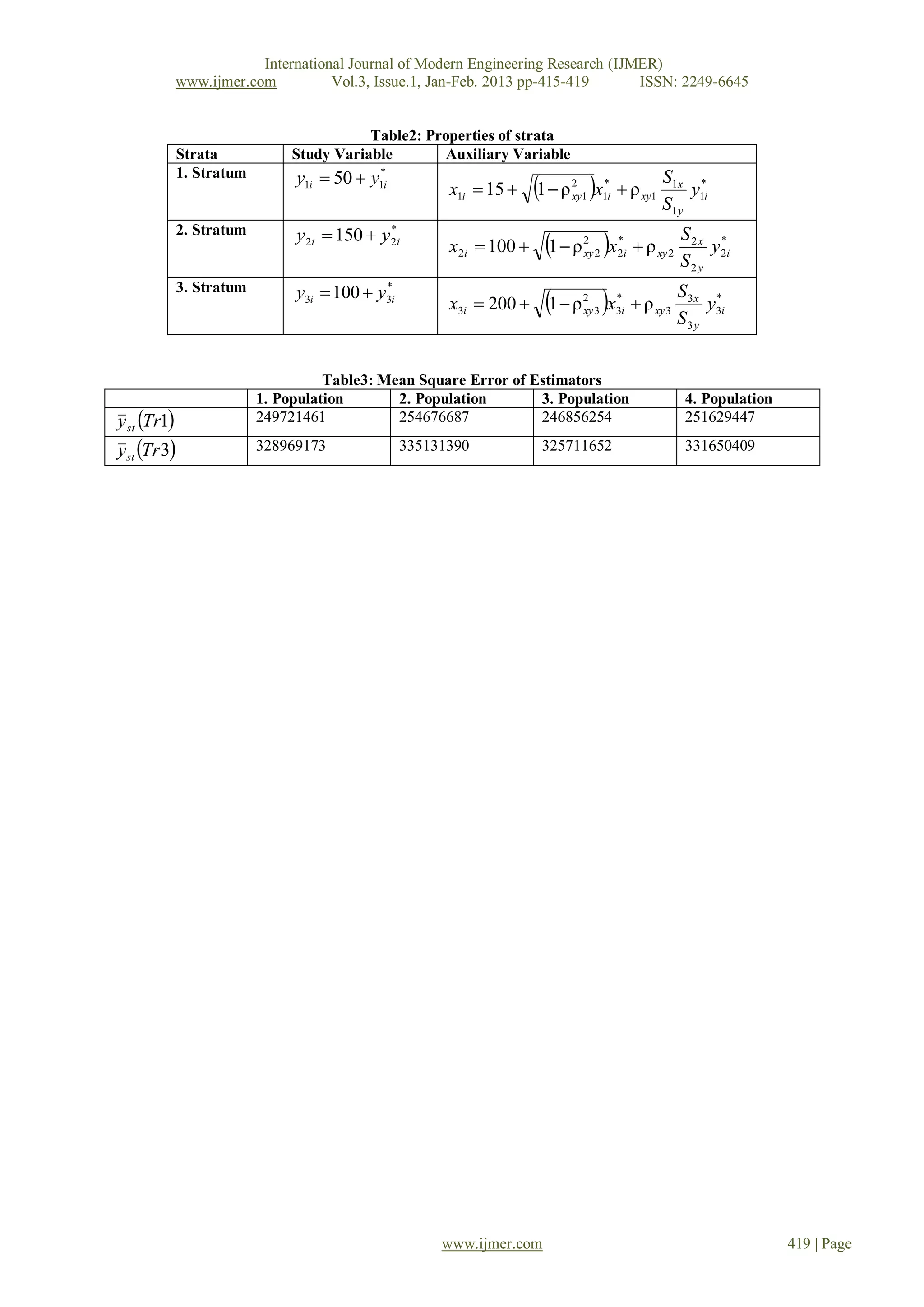
MSE  y st α   k  , α  Tr, Tr
N
 
n
 
It should be mentioned that in the case of distance function L and L , the iterative procedure for finding weights
from the Lagrange equations doesn’t converge for all selected samples. (See Pumputis (2005)). So we didn’t give simulation
results for L and L .
The simulation study shows that calibration estimator using distance measure L are highly efficient than using
distance measure L .
IV. CONCLUSION
In this study we derived some new weights using different distance measures theoretically in stratified random
sampling. The performance of the weights are compared with a simulation study.
REFERENCES
[1] Arnab, R., Singh, S., 2005, A note on variance estimation for the generalized regression predictor, Australian and New Zealand
Journal of Statistics, 47, 2, 231–234.
[2] Deville, J.C., Sarndal, C.E., 1992, Calibration estimators in survey sampling, Journal of the American Statistical Association, 87,
376-382.
[3] Estevao, V.M., Sarndal, C.E., 2000, A functional form approach to calibration, Journal of Official Statistics, 16, 379-399.
[4] Farrell, P.J., Singh, S., 2005, Model-assisted higher order calibration of estimators of variance, Australian and New Zealand Journal
of Statistics, 47, 3, 375–383.
[5] Kim, J.M., Sungur, E.A., Heo T.Y., 2007, Calibration approach estimators in stratified sampling, Statistics and Probability Letters,
77, 1, 99-103.
[6] Kim, J.K., Park, M., 2010, Calibration estimation in survey sampling, International Statistical Review, 78, 1, 21-29.
[7] Koyuncu, N., 2012, Application of Calibration Method to Estimators in Sampling Theory, Hacettepe University Department of
Statistics, PhD. Thesis.
[8] Pumputis D. Calibrated estimators under different distance measures. Proceedings of the Workshop on Survey Sampling Theory and
Methodology, 2005, p. 137–141. ISBN 9955-588-87-X.
[9] Tracy, D.S., Singh, S., Arnab, R., 2003, Note on calibration in stratified and double sampling, Survey Methodology, 29, 99–104.
Table 1: Parameters and distributions of study and auxiliary variables
Parameters and distributions of the Parameters and distributions of the
study variable auxiliary variable
1. Population, h  , , 
 
 
f y hi 
*
Γ.
y hi .e  yhi
* *
 
f xhi 
*
Γ.
xhi.e  xhi
* *
2. Population, h  , , 

 
*

 
xhi
y hi.e  yhi 
*
f y hi 
* *

Γ.
*
f x hi e
π
3. Population, h  , , 

 
*

 
y hi
xhi.e  xhi
*

f xhi 
* *
Γ.
* 
f y hi e
π
4. Population, h  , , 
* *

 
xhi

 
y hi
 
*  * 
f y e f x hi e
π
hi
π
www.ijmer.com 418 | Page

5. International Journal of Modern Engineering Research (IJMER)
www.ijmer.com Vol.3, Issue.1, Jan-Feb. 2013 pp-415-419 ISSN: 2249-6645
Table2: Properties of strata
Strata Study Variable Auxiliary Variable
yi    yi
  ρ x
1. Stratum *
Sx *

xi    xy
*
i  ρ xy yi
S y
yi    yi
  ρ x
2. Stratum *
Sx *

xi    xy 
*
i  ρ xy  y i
S y
yi    yi
 
3. Stratum *
S x *
xi      ρ   xi  ρ xy 
xy
*
yi
S y
Table3: Mean Square Error of Estimators
1. Population 2. Population 3. Population 4. Population
y st Tr 249721461 254676687 246856254 251629447
yst Tr  328969173 335131390 325711652 331650409
www.ijmer.com 419 | Page