Downloaded 137 times


![36 | COPPER FOR BUSBARS
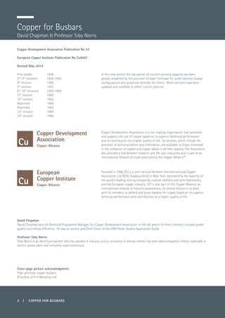
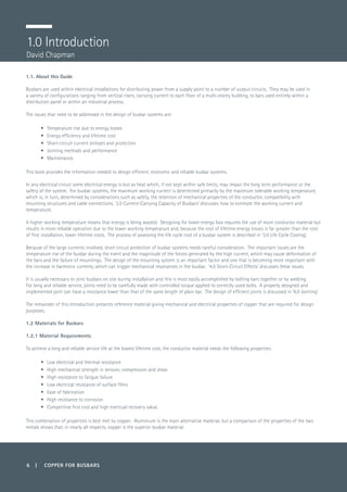
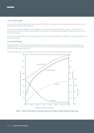
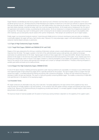
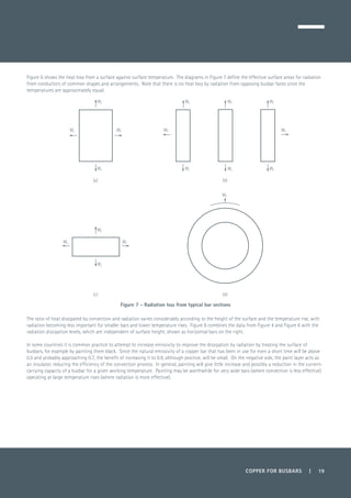
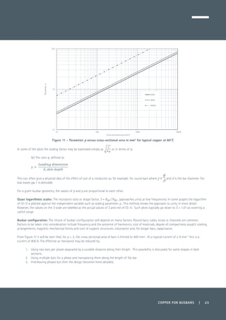
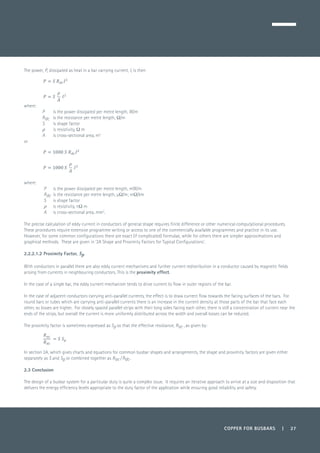
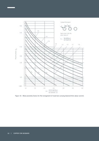
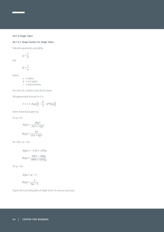
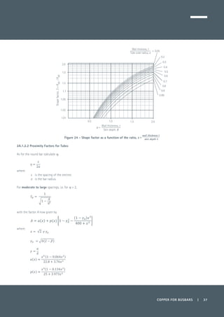
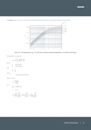
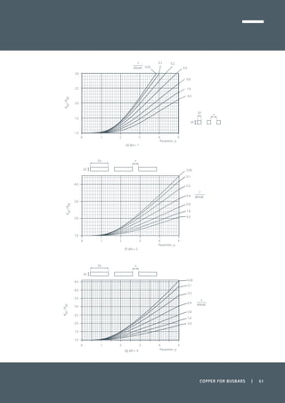
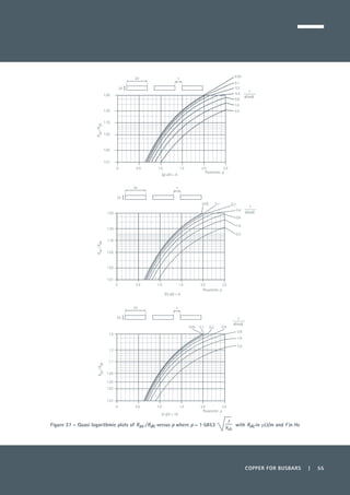
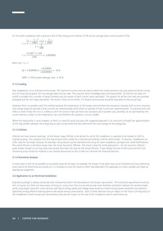
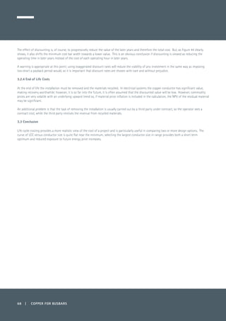
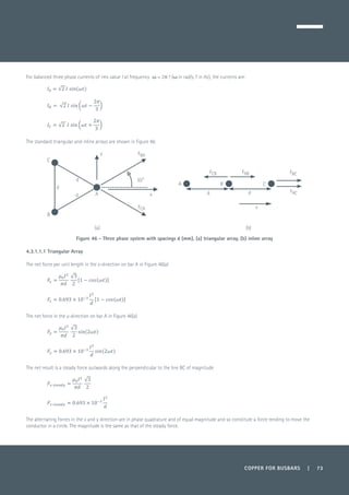
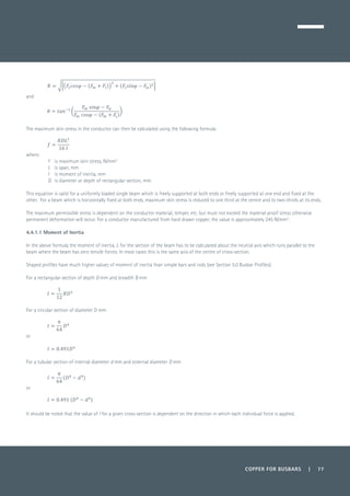
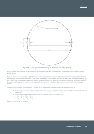
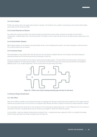
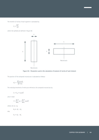
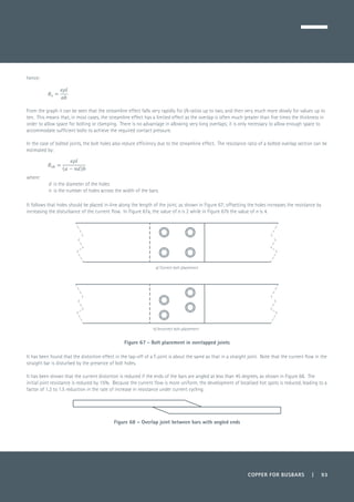
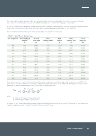
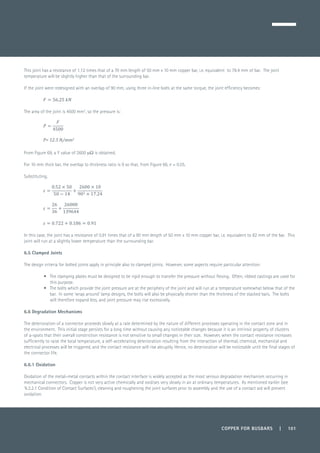
Figure 22 - Shape factor for tubes
Figure 23 - The shape factor computed from the Bessel function formula using √(f/rdc) as the frequency parameter
10 2 3 4 5 6 7
1.2
1.0
1.4
1.6
1.8
2.0
f, Hz
Rdc
, µ /m[ ]√
0.15
0.125
0.10
0.075
0.05
0.20
0.25
0.99 0.8 0.7 0.300.40.50.6
Shapefactor,S=Rac/Rdc
Wall thickness, t
Tube outer radius, a
=
1 2 3 4 5 6 7
1.02
1.01
1.05
1.1
1.2
1.5
2.0
0
0.99 0.8 0.7 0.4
0.15
0.10
0.075
0.05
0.20
0.300.50.6
Wall thickness, t
Tube outer radius, a
=
Shapefactor,S=Rac/Rdc
f, Hz
Rdc
, µ /m[ ]√](https://image.slidesharecdn.com/3w5zxph9teql5hsdgrot-140601063439-phpapp02/85/Copper-for-Busbars-36-320.jpg)
![COPPER FOR BUSBARS | 43
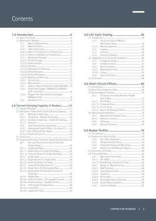
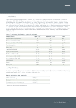
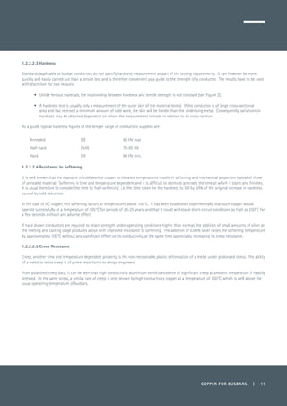
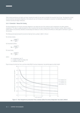
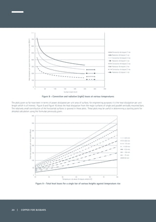
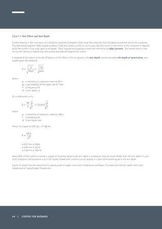
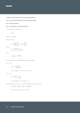
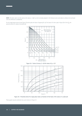
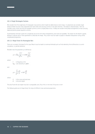
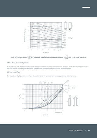
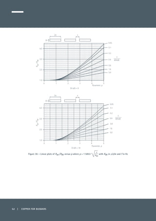
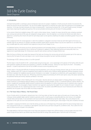
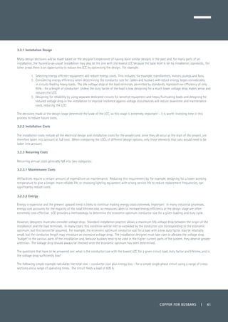
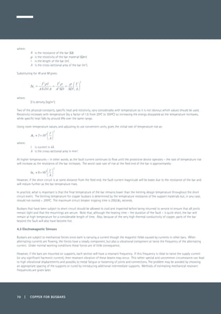
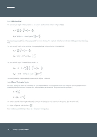
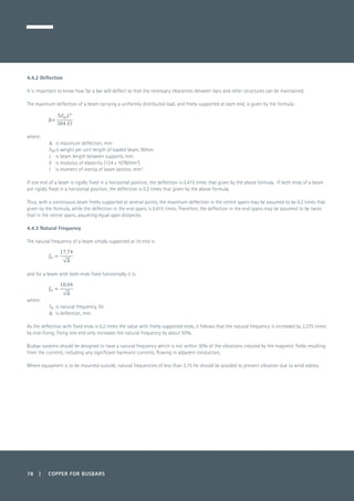
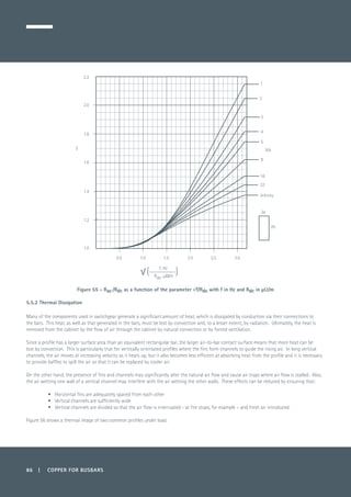
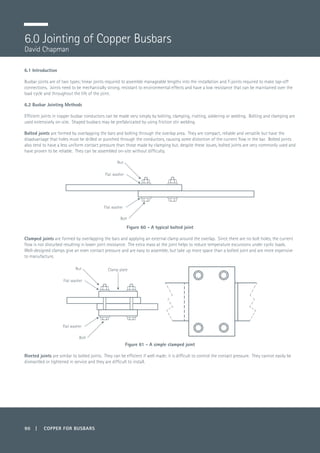
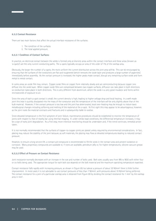
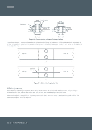
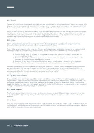
Figure 30 - Rac /Rdc as a function of the parameter √f/Rdc
Figure 31 - Rac /Rdc as a function of the parameter √f/Rdc . The range of the parameter is narrower than in the previous figure
1.0
2b
2a
1
2
3
4
8
16
32
Infinity
5
b/a
0.5 1.0 1.5 2.0 2.5 3.0
1.2
1.4
1.6
1.8
2.0
2.2
f, Hz
Rdc
, µ /m[ ]√
Rac/Rdc
2a
1
2
3
4
7
16
32
Infinity
5
2b
0.5 1.0 1.5 2.0
1.05
1.00
1.10
1.15
1.20
1.25
1.30
1.35
1.40
10
64
b/a
f, Hz
Rdc
, µ /m[ ]√
Rac/Rdc](https://image.slidesharecdn.com/3w5zxph9teql5hsdgrot-140601063439-phpapp02/85/Copper-for-Busbars-43-320.jpg)
![44 | COPPER FOR BUSBARS
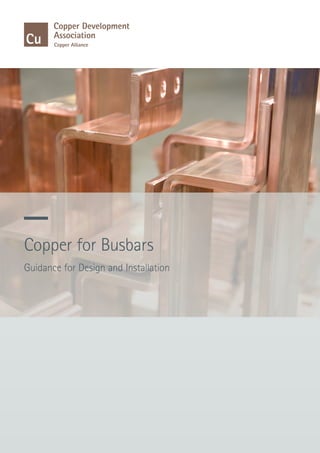
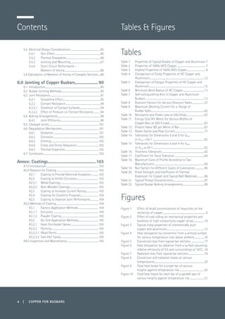
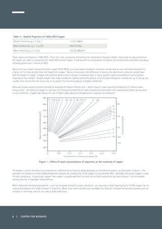
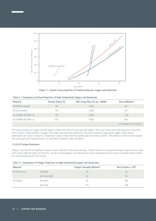
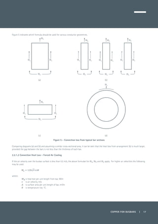
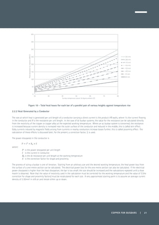
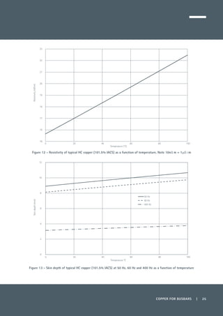
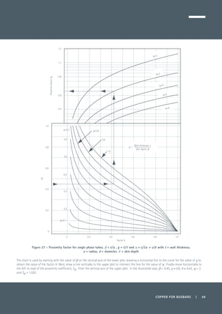
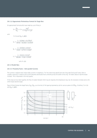
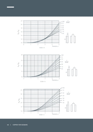
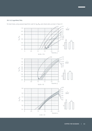
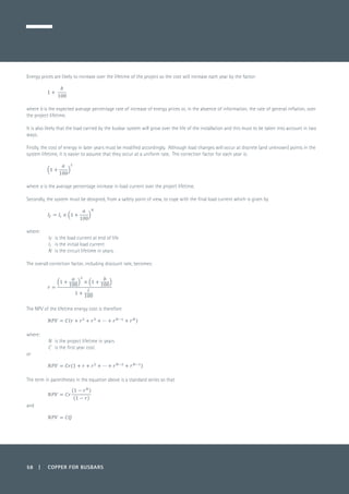
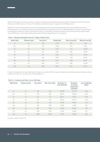
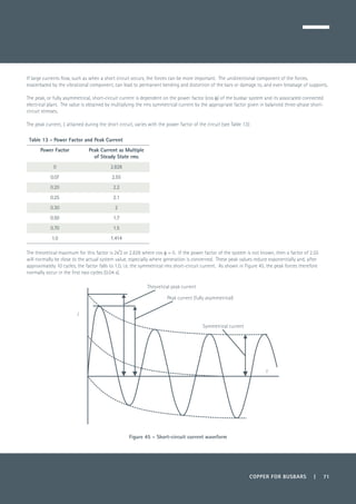
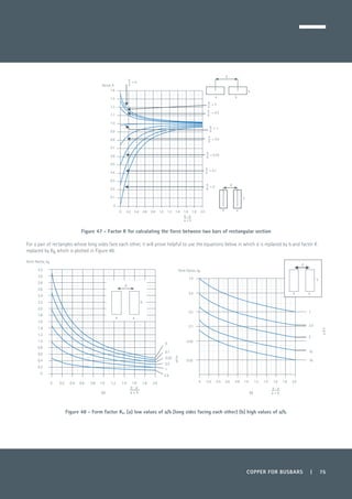
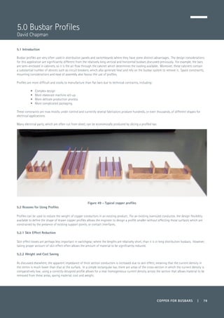
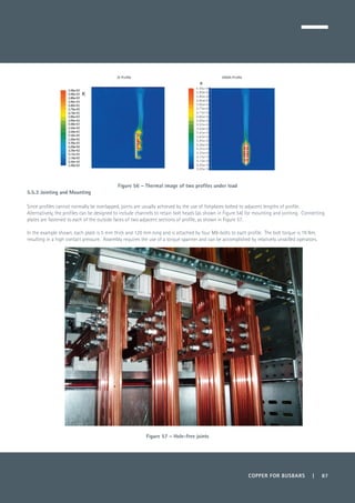
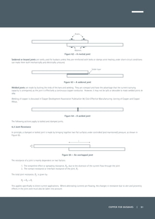
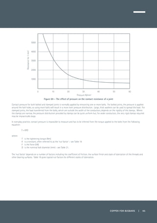
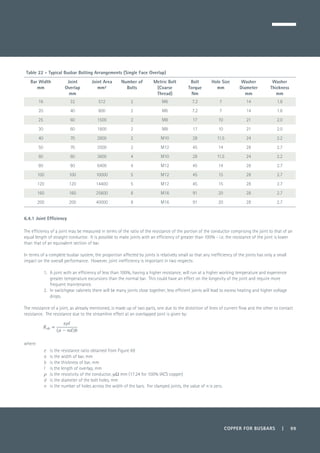
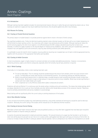
At low values of p the curves for the different aspects ratios cross, as illustrated in Figure 32.
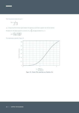
Figure 32 - Shape factor, Rac /Rdc , as a function of the parameter √f/Rdc .
Note the logarithmic scale for the shape factor and that the lines for constant b/a cross.
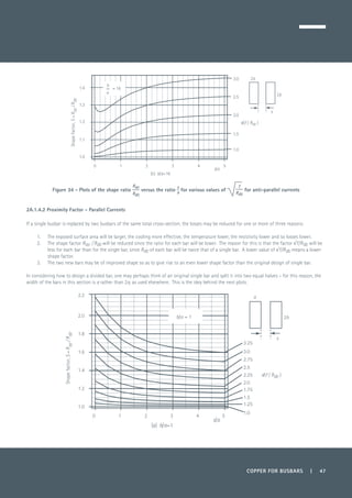
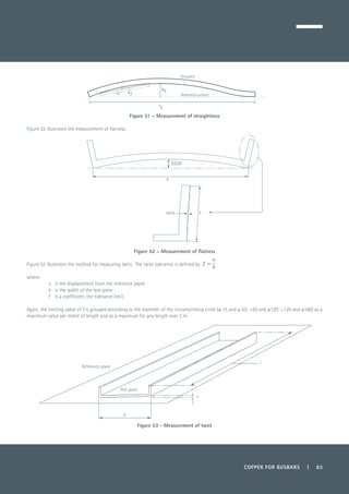
Figure 33 - Shape factor versus 2b/d for various values of b/a
For values of √(f/Rdc) < 1.25 the thin sectioned bar has a slightly higher shape factor than the square conductor, whereas for higher values a thin
shape gives a lower shape factor. For copper at 20˚C with r = 17 nΩ m the transitional cross-sectional area is about 500 mm2
; i.e. in old units,
about 1 sq in. One may, however, prefer a thin strip of say 6 mm by 80 mm, which is more readily cooled because it has a larger vertical flat face.
The increase in losses is of the order of one percent.
b/a = 5 32 Inf161 3
1.0 1.2 1.4 1.6 1.8
1.03
1.02
1.05
1.07
1.10
1.15
1.20
Rac/Rdc
f, Hz
Rdc
, µ /m[ ]√
5 10 15 20 25 30
1.02
1.01
1.05
1.10
1.20
1.50
2.00
Long side, 2b
Skin depth, δ
32
1610754321b/a =
64
24
0
Rac/Rdc](https://image.slidesharecdn.com/3w5zxph9teql5hsdgrot-140601063439-phpapp02/85/Copper-for-Busbars-44-320.jpg)

![COPPER FOR BUSBARS | 63
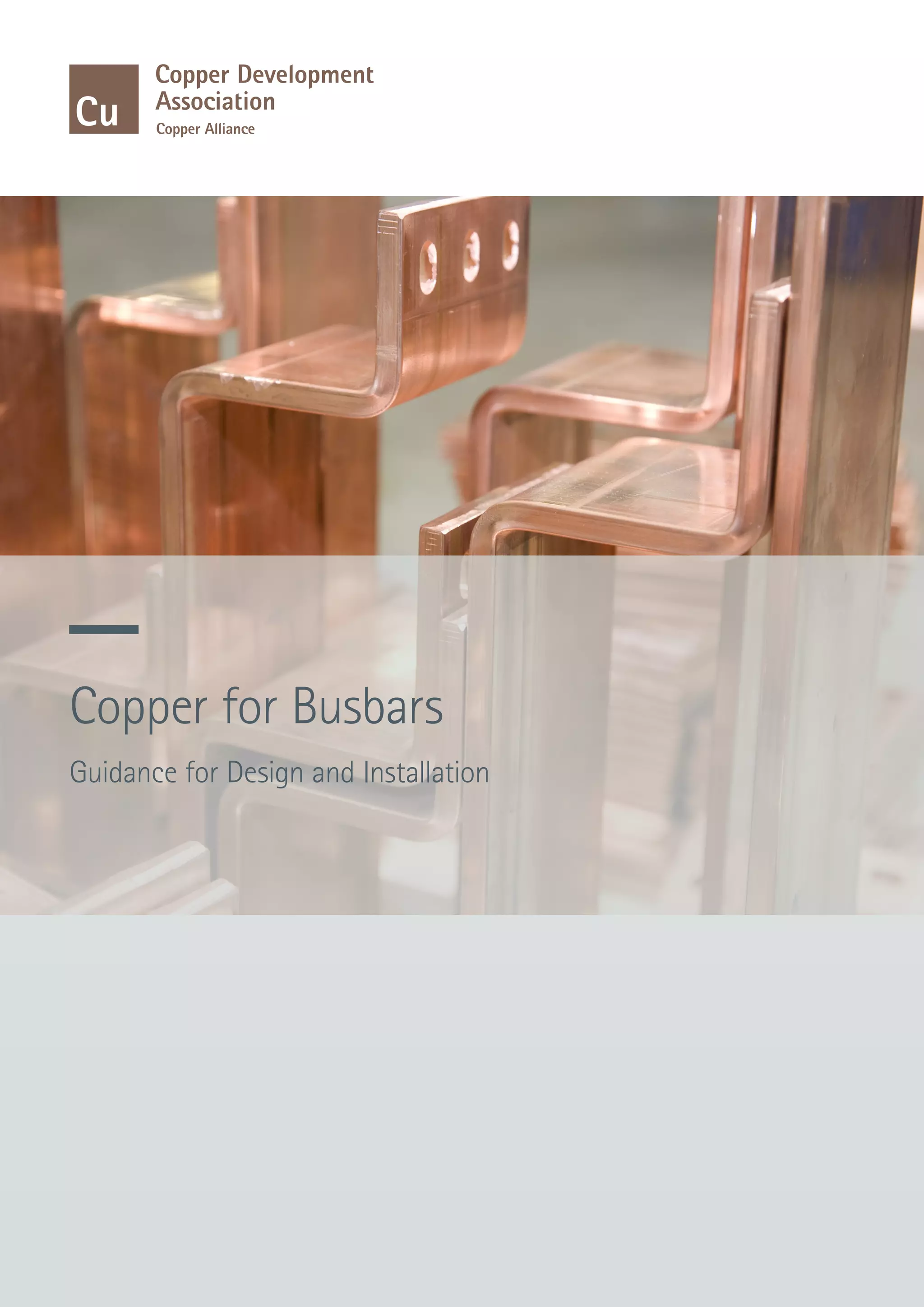
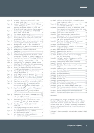
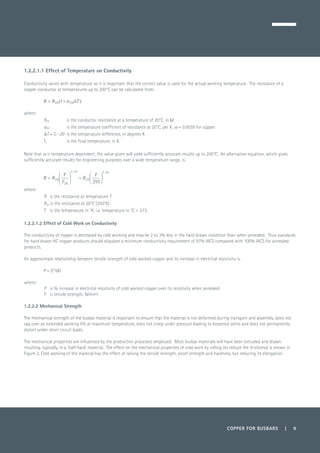
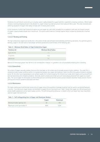
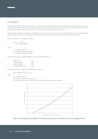
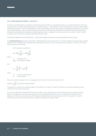
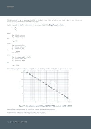
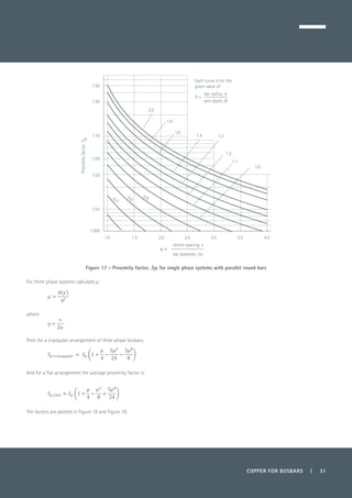
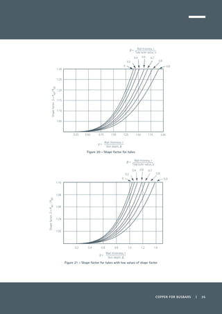
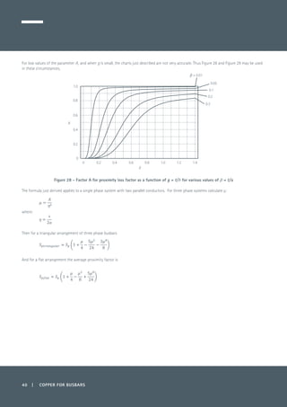
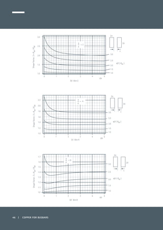
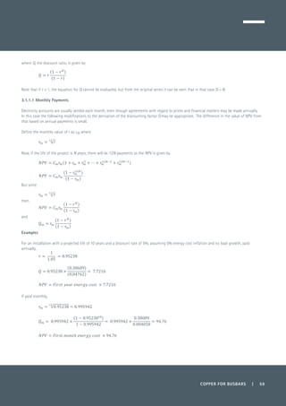
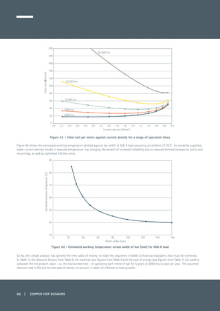
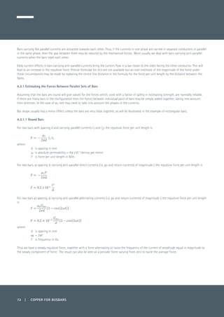
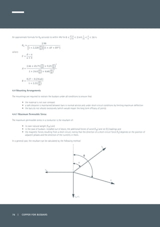
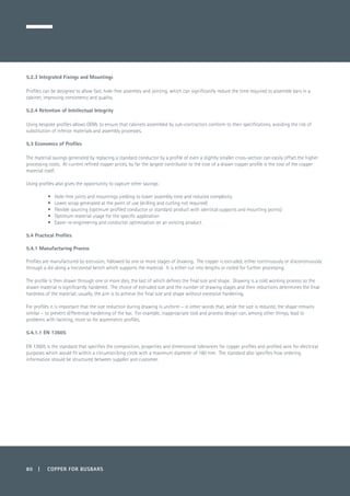
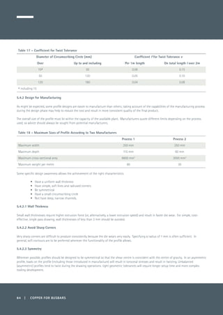
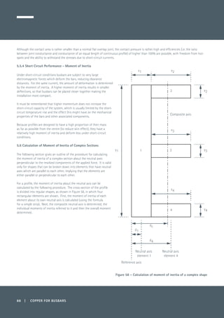
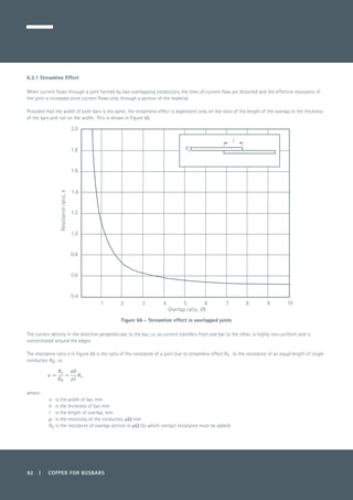
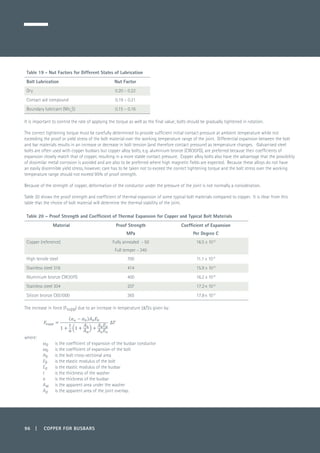
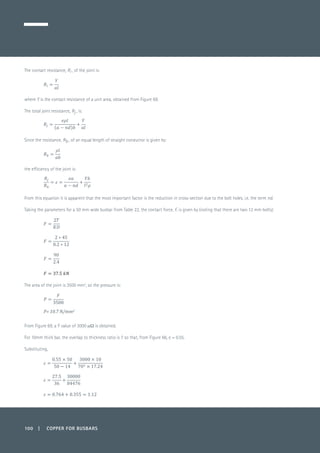
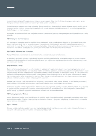
Figure 38 - Power loss versus width for 6.3 mm thick copper bars
The power loss needs to be expressed in terms of money by converting to energy loss (by multiplying by the operation time) and multiplying by the
cost of energy. For the purposes of this exercise, the cost of energy is assumed to be 0.15 Euro per kWh. Table 11 and Figure 39 show the energy
cost per metre for a range of operation times.
Table 11 – Energy Cost per Metre for Various Widths of Copper Bars at 500 A Load
Cost of Energy (€ per metre)
Width (mm) 2000 hrs 5000 hrs 10 000 hrs 20 000 hrs 50 000 hrs
25 10.36 25.89 51.79 103.58 258.94
31.5 7.85 19.62 39.24 78.49 196.21
40 5.97 14.93 29.86 59.73 149.32
50 4.66 11.66 23.31 46.62 116.56
63 3.63 9.09 18.17 36.35 90.87
80 2.84 7.10 14.21 28.42 71.04
100 2.25 5.62 11.24 22.49 56.22
125 1.77 4.43 8.86 17.73 44.32
160 1.38 3.46 6.92 13.85 34.62
0.00
5.00
10.00
15.00
20.00
25.00
30.00
35.00
40.00
0 20 40 60 80 100 120 140 160
Powerlosspermetrelengthat500Amp(W)
Width of copper bar (mm) [Thickness 6.3 mm]](https://image.slidesharecdn.com/3w5zxph9teql5hsdgrot-140601063439-phpapp02/85/Copper-for-Busbars-63-320.jpg)
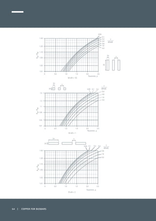
![64 | COPPER FOR BUSBARS
Figure 39 – Cost of energy loss per metre versus width for 6.3 mm thick copper bars for a range of operating times
By comparison with the material costs in Table 9 it is immediately apparent that, for any significant operational life, the cost of energy is by far the
dominant element in the total cost of the system. Consider, for example, the 5000 hour operation case.
Figure 40 - Total cost per metre versus bar width for 5000 hours operation at 500 A load
Figure 40 shows the total cost, material cost (from Table 9) and energy cost (from Table 11) per metre of bar. As the width of the bar increases, the
cost of material increases linearly, while the cost of energy decreases super inversely as the resistance and temperature decrease. The total cost
curve shows a clear minimum where the total cost is optimised between investment cost (material) and operating costs (energy).
Because the cost of energy is proportional to operation time, the optimum bar width also increases with operation time, as shown in Figure 41,
which plots the total cost per metre of bar for a range of operation times. As operation time increases, the optimum bar width increases.
0
50
100
150
200
250
300
0 20 40 60 80 100 120 140 160
Costofenergy(€)
Width of copper bar (mm) [Thickness 6.3 mm]
50 000 hrs
20 000 hrs
10 000 hrs
5000 hrs
2000 hrs
0
10
20
30
40
50
60
0 20 40 60 80 100 120 140 160
Cost(€)
Width of copper bar (mm) [Thickness 6.3 mm]
Cost of material (€)
Cost of energy losses over 5000 hours (€)
Total cost over 5000 hours (€)
Optimum cross-section](https://image.slidesharecdn.com/3w5zxph9teql5hsdgrot-140601063439-phpapp02/85/Copper-for-Busbars-64-320.jpg)
![COPPER FOR BUSBARS | 65
Figure 41 - Total cost per metre of bar versus bar width for a range of operating times
Figures 40 and 41 illustrate two important points:
At the minimum bar size – i.e. the size that would be selected by conventional methods – the cost of lifetime energy is many times the cost of the
conductor; a factor of approximately 3.4 at 5000 hours. In fact, such a bar wastes its own cost in energy in less than 1500 operational hours, at
the material and energy costs used in this example.
The minimum of the total cost curve is shallow, meaning that there is some latitude for judgement in the selection of the final size with a high
degree of confidence in the outcome. For example, if the operational hours were not well known, but could be expected to be between 20 000 and
50 000 hours, a 100 mm bar could be confidently selected, being a little over optimum size for 20 000 hours and a little under optimum size for
50 000 hours.
Figure 42 is an alternative plot of the data in Figure 41 showing the optimum current density for a range of operating hours. As would be
expected, the optimum current density reduces as operating hours increase.
0.00
20.00
40.00
60.00
80.00
100.00
120.00
140.00
160.00
180.00
200.00
0 20 40 60 80 100 120 140 160
Totalcost(€)
Width of copper bar (mm) [Thickness 6.3 mm]
50 000 hours
20 000 hours
10 000 hours
5000 hours
2000 hours](https://image.slidesharecdn.com/3w5zxph9teql5hsdgrot-140601063439-phpapp02/85/Copper-for-Busbars-65-320.jpg)
![COPPER FOR BUSBARS | 67
In this case, because the energy is paid for throughout the operating time, no discount is applied to Year 0. Local accounting practice may require
discounting to be applied to Year 0 in some cases.
Table 12 – Present Value (€) per Metre of Bar
Discount Factor
Cost of Energy (2000 hours per year)
Total
Year 0 Year 1 Year 2 Year 3 Year 4 Total
1 0.952 0.907 0.864 0.823
Bar Width
(mm)
Power Loss
per Metre
(watt)
Cost of Bar
(euro)
25 34.53 7.518 10.36 9.8627 9.3965 8.9510 8.5263 47.10 54.61
31.5 26.16 9.472 7.85 7.4732 7.1200 6.7824 6.4606 35.69 45.16
40 19.91 12.029 5.97 5.6834 5.4148 5.1581 4.9133 27.14 39.17
50 15.54 15.036 4.66 4.4363 4.2266 4.0262 3.8352 21.18 36.22
63 12.12 18.945 3.63 3.4558 3.2924 3.1363 2.9875 16.50 35.45
80 9.41 24.057 2.82 2.6846 2.5577 2.4365 2.3209 12.82 36.88
100 7.45 30.071 2.24 2.1325 2.0317 1.9354 1.8435 10.18 40.25
125 5.93 37.589 1.78 1.6946 1.6145 1.5379 1.4649 8.09 45.68
160 4.62 48.114 1.38 1.3138 1.2517 1.1923 1.1357 6.27 54.39
Figure 44 shows the comparison between the discounted and non-discounted cost, this time for a 10 year life.
Figure 44 - Cost per metre (€) against bar width for a) 20 000 hours operation without discount and
b) 2000 hours per year for 10 years at 5% discount
0
20
40
60
80
100
120
0 20 40 60 80 100 120 140 160
Costpermetre(€)
Width of bar (mm) [Thickness 6.3 mm]
20 000 hours (No discount)
2000 hours per year for 10 years at 5% discount](https://image.slidesharecdn.com/3w5zxph9teql5hsdgrot-140601063439-phpapp02/85/Copper-for-Busbars-67-320.jpg)


The document provides comprehensive guidance on the design and installation of copper busbars, emphasizing their superior technical performance and applications. It includes calculations for current-carrying capacity, material requirements, life cycle costing, short-circuit effects, and jointing methods. Revised in May 2014, this edition simplifies complex calculations and updates sections to better reflect current practices in the industry.