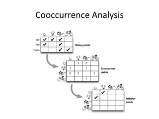
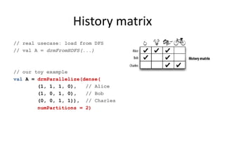
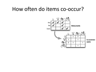
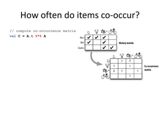
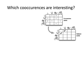
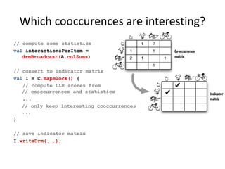
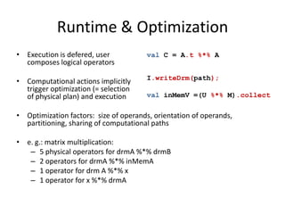
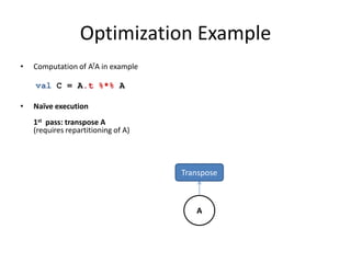
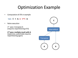
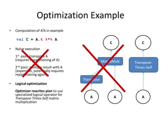
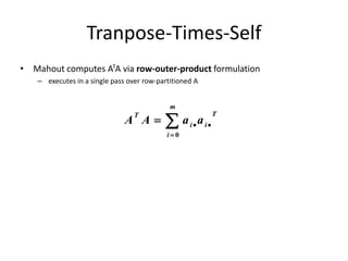
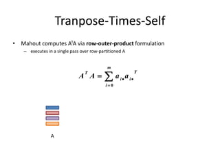
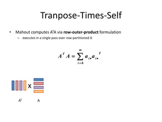
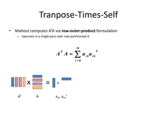
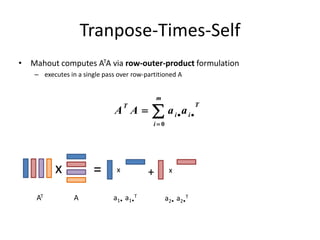
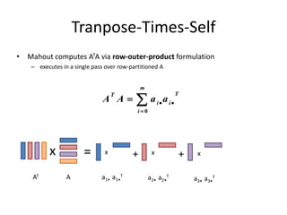
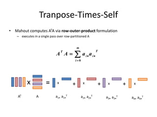
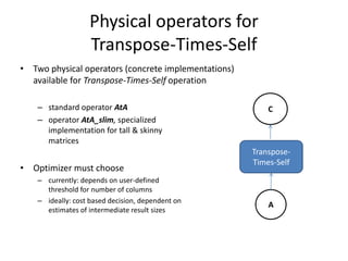
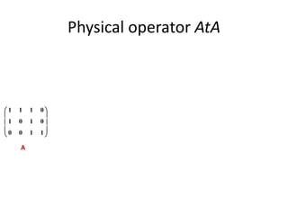
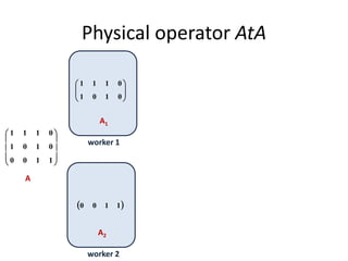
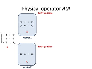
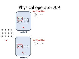
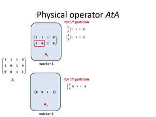
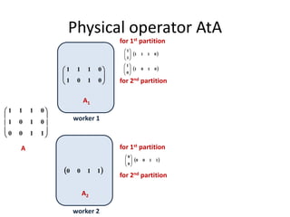
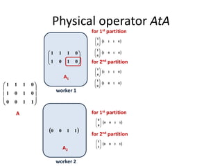
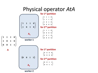
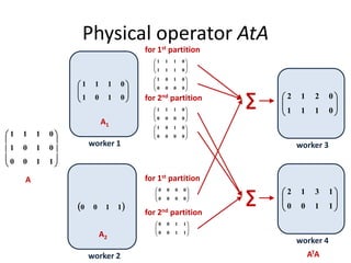
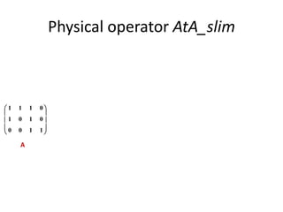
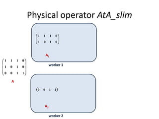
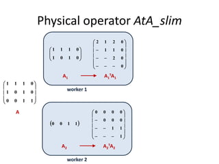
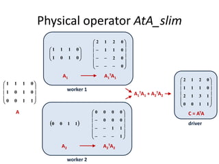
Co-occurrence-based recommendations
with Mahout, Scala & Spark
Sebastian Schelter
@sscdotopen
BigData Beers
05/29/2014
available for free at
http://www.mapr.com/practical-machine-learning
Cooccurrence Analysis
History matrix
// real usecase: load from DFS
// val A = drmFromHDFS(...)
// our toy example
val A = drmParallelize(dense(
(1, 1, 1, 0), // Alice
(1, 0, 1, 0), // Bob
(0, 0, 1, 1)), // Charles
numPartitions = 2)
How often do items co-occur?
// compute co-occurrence matrix
val C = A.t %*% A
Which cooccurences are interesting?
// compute some statistics
val interactionsPerItem =
drmBroadcast(A.colSums)
// convert to indicator matrix
val I = C.mapBlock() {
// compute LLR scores from
// cooccurrences and statistics
...
// only keep interesting cooccurrences
...
}
// save indicator matrix
I.writeDrm(...);
Cooccurrence Analysis
prototype available
• MAHOUT-1464 provides full-fledged cooccurrence analysis protoype
– applies selective downsampling to make computation tractable
– support for cross-recommendations in datasets with multiple
interaction types, e.g.
• “people who watch this video also watch those videos”
• “people who enter this search query watch those videos”
– code to run this on the Movielens and Epinions datasets
• future plan: easy indexing of indicator matrix with Apache Solr to allow
for search-as-recommendation deployments
– prototype for MR code already existing at https://github.com/pferrel/solr-recommender
– integration is in the works
Under the covers
Underlying systems
• currently: runtime based on Apache Spark
– fast and expressive cluster
computing system
– general computation graphs,
in-memory primitives, rich API,
interactive shell
• potentially supported in the future:
• Apache Flink (formerly: “Stratosphere”)
• H20
Runtime & Optimization
• Execution is defered, user
composes logical operators
• Computational actions implicitly
trigger optimization (= selection
of physical plan) and execution
• Optimization factors: size of operands, orientation of operands,
partitioning, sharing of computational paths
• e. g.: matrix multiplication:
– 5 physical operators for drmA %*% drmB
– 2 operators for drmA %*% inMemA
– 1 operator for drm A %*% x
– 1 operator for x %*% drmA
val C = A.t %*% A
I.writeDrm(path);
val inMemV =(U %*% M).collect
Optimization Example
• Computation of ATA in example
• Naïve execution
1st pass: transpose A
(requires repartitioning of A)
2nd pass: multiply result with A
(expensive, potentially requires
repartitioning again)
• Logical optimization:
rewrite plan to use specialized
logical operator for
Transpose-Times-Self matrix
multiplication
val C = A.t %*% A
Transpose
A
Optimization Example
• Computation of ATA in example
• Naïve execution
1st pass: transpose A
(requires repartitioning of A)
2nd pass: multiply result with A
(expensive, potentially requires
repartitioning again)
• Logical optimization:
rewrite plan to use specialized
logical operator for
Transpose-Times-Self matrix
multiplication
val C = A.t %*% A
Transpose
MatrixMult
A A
C
Optimization Example
• Computation of ATA in example
• Naïve execution
1st pass: transpose A
(requires repartitioning of A)
2nd pass: multiply result with A
(expensive, potentially requires
repartitioning again)
• Logical optimization
Optimizer rewrites plan to use
specialized logical operator for
Transpose-Times-Self matrix
multiplication
val C = A.t %*% A
Transpose
MatrixMult
A A
C
Transpose-
Times-Self
A
C
Tranpose-Times-Self
• Mahout computes ATA via row-outer-product formulation
– executes in a single pass over row-partitioned A




m
i
T
ii
T
aaAA
0
Tranpose-Times-Self
• Mahout computes ATA via row-outer-product formulation
– executes in a single pass over row-partitioned A




m
i
T
ii
T
aaAA
0
A
Tranpose-Times-Self
• Mahout computes ATA via row-outer-product formulation
– executes in a single pass over row-partitioned A




m
i
T
ii
T
aaAA
0
x
AAT
Tranpose-Times-Self
• Mahout computes ATA via row-outer-product formulation
– executes in a single pass over row-partitioned A




m
i
T
ii
T
aaAA
0
x = x
AAT a1• a1•
T
Tranpose-Times-Self
• Mahout computes ATA via row-outer-product formulation
– executes in a single pass over row-partitioned A




m
i
T
ii
T
aaAA
0
x = x + x
AAT a1• a1•
T
a2• a2•
T
Tranpose-Times-Self
• Mahout computes ATA via row-outer-product formulation
– executes in a single pass over row-partitioned A




m
i
T
ii
T
aaAA
0
x = x + +x x
AAT a1• a1•
T
a2• a2•
T
a3• a3•
T
Tranpose-Times-Self
• Mahout computes ATA via row-outer-product formulation
– executes in a single pass over row-partitioned A




m
i
T
ii
T
aaAA
0
x = x + + +x x x
AAT a1• a1•
T
a2• a2•
T
a3• a3•
T
a4• a4•
T
Physical operators for
Transpose-Times-Self
• Two physical operators (concrete implementations)
available for Transpose-Times-Self operation
– standard operator AtA
– operator AtA_slim, specialized
implementation for tall & skinny
matrices
• Optimizer must choose
– currently: depends on user-defined
threshold for number of columns
– ideally: cost based decision, dependent on
estimates of intermediate result sizes
Transpose-
Times-Self
A
C
Physical operators for the
distributed computation of ATA
Physical operator AtA










1100
0101
0111
A
A2
 1100
Physical operator AtA










1100
0101
0111
A1
A
worker 1
worker 2






0101
0111
A2
 1100
Physical operator AtA










1100
0101
0111
A1
A
worker 1
worker 2






0101
0111
for 1st partition
for 1st partition
A2
 1100
Physical operator AtA










1100
0101
0111
A1
A
worker 1
worker 2






0101
0111
 0111
1
1






 1100
0
0






for 1st partition
for 1st partition
A2
 1100
Physical operator AtA










1100
0101
0111
A1
A
worker 1
worker 2






0101
0111
 0111
1
1






 1100
0
0






for 1st partition
for 1st partition
 0101
0
1






A2
 1100
Physical operator AtA










1100
0101
0111
A1
A
worker 1
worker 2






0101
0111
 0111
1
1






 1100
0
0






for 1st partition
for 1st partition
 0101
0
1






for 2nd partition
for 2nd partition
A2
 1100
Physical operator AtA










1100
0101
0111
A1
A
worker 1
worker 2






0101
0111
 0111
1
1






 1100
0
0






for 1st partition
for 1st partition
 0101
0
1






 0111
0
1






for 2nd partition
 1100
1
1






for 2nd partition
A2
 1100
Physical operator AtA










1100
0101
0111
A1
A
worker 1
worker 2






0101
0111
 0111
1
1






 1100
0
0






for 1st partition
for 1st partition
 0101
0
1






 0111
0
1






for 2nd partition
 0101
0
1






 1100
1
1






for 2nd partition
A2
 1100
Physical operator AtA










1100
0101
0111
A1
A
worker 1
worker 2






0101
0111






0111
0111






0000
0000
for 1st partition
for 1st partition






0000
0101






0000
0111
for 2nd partition






0000
0101






1100
1100
for 2nd partition






0111
0212
worker 3






1100
1312
worker 4
∑
∑
ATA
Physical operator AtA_slim










1100
0101
0111
A
A2
 1100
Physical operator AtA_slim










1100
0101
0111
A1
A
worker 1
worker 2






0101
0111
A2
TA2A2
 1100

















1
11
000
0000
Physical operator AtA_slim










1100
0101
0111
A1
TA1A1
A
worker 1
worker 2






0101
0111

















0
02
011
0212
A2
TA2A2
 1100

















1
11
000
0000
Physical operator AtA_slim










1100
0101
0111
A1
TA1A1
A C = ATA
worker 1
worker 2
A1
TA1 + A2
TA2
driver






0101
0111

















0
02
011
0212














1100
1312
0111
0212
Thank you. Questions?
Overview of Mahout‘s Scala & Spark Bindings:
http://s.apache.org/mahout-spark
Tutorial on playing with Mahout‘s Spark shell
http://s.apache.org/mahout-spark-shell

Co-occurrence Based Recommendations with Mahout, Scala and Spark

  • 1.
    Co-occurrence-based recommendations with Mahout,Scala & Spark Sebastian Schelter @sscdotopen BigData Beers 05/29/2014
  • 2.
    available for freeat http://www.mapr.com/practical-machine-learning
  • 3.
  • 4.
    History matrix // realusecase: load from DFS // val A = drmFromHDFS(...) // our toy example val A = drmParallelize(dense( (1, 1, 1, 0), // Alice (1, 0, 1, 0), // Bob (0, 0, 1, 1)), // Charles numPartitions = 2)
  • 5.
    How often doitems co-occur?
  • 6.
    How often doitems co-occur? // compute co-occurrence matrix val C = A.t %*% A
  • 7.
  • 8.
    Which cooccurences areinteresting? // compute some statistics val interactionsPerItem = drmBroadcast(A.colSums) // convert to indicator matrix val I = C.mapBlock() { // compute LLR scores from // cooccurrences and statistics ... // only keep interesting cooccurrences ... } // save indicator matrix I.writeDrm(...);
  • 9.
    Cooccurrence Analysis prototype available •MAHOUT-1464 provides full-fledged cooccurrence analysis protoype – applies selective downsampling to make computation tractable – support for cross-recommendations in datasets with multiple interaction types, e.g. • “people who watch this video also watch those videos” • “people who enter this search query watch those videos” – code to run this on the Movielens and Epinions datasets • future plan: easy indexing of indicator matrix with Apache Solr to allow for search-as-recommendation deployments – prototype for MR code already existing at https://github.com/pferrel/solr-recommender – integration is in the works
  • 10.
  • 11.
    Underlying systems • currently:runtime based on Apache Spark – fast and expressive cluster computing system – general computation graphs, in-memory primitives, rich API, interactive shell • potentially supported in the future: • Apache Flink (formerly: “Stratosphere”) • H20
  • 12.
    Runtime & Optimization •Execution is defered, user composes logical operators • Computational actions implicitly trigger optimization (= selection of physical plan) and execution • Optimization factors: size of operands, orientation of operands, partitioning, sharing of computational paths • e. g.: matrix multiplication: – 5 physical operators for drmA %*% drmB – 2 operators for drmA %*% inMemA – 1 operator for drm A %*% x – 1 operator for x %*% drmA val C = A.t %*% A I.writeDrm(path); val inMemV =(U %*% M).collect
  • 13.
    Optimization Example • Computationof ATA in example • Naïve execution 1st pass: transpose A (requires repartitioning of A) 2nd pass: multiply result with A (expensive, potentially requires repartitioning again) • Logical optimization: rewrite plan to use specialized logical operator for Transpose-Times-Self matrix multiplication val C = A.t %*% A
  • 14.
    Optimization Example • Computationof ATA in example • Naïve execution 1st pass: transpose A (requires repartitioning of A) 2nd pass: multiply result with A (expensive, potentially requires repartitioning again) • Logical optimization: rewrite plan to use specialized logical operator for Transpose-Times-Self matrix multiplication val C = A.t %*% A Transpose A
  • 15.
    Optimization Example • Computationof ATA in example • Naïve execution 1st pass: transpose A (requires repartitioning of A) 2nd pass: multiply result with A (expensive, potentially requires repartitioning again) • Logical optimization: rewrite plan to use specialized logical operator for Transpose-Times-Self matrix multiplication val C = A.t %*% A Transpose MatrixMult A A C
  • 16.
    Optimization Example • Computationof ATA in example • Naïve execution 1st pass: transpose A (requires repartitioning of A) 2nd pass: multiply result with A (expensive, potentially requires repartitioning again) • Logical optimization Optimizer rewrites plan to use specialized logical operator for Transpose-Times-Self matrix multiplication val C = A.t %*% A Transpose MatrixMult A A C Transpose- Times-Self A C
  • 17.
    Tranpose-Times-Self • Mahout computesATA via row-outer-product formulation – executes in a single pass over row-partitioned A     m i T ii T aaAA 0
  • 18.
    Tranpose-Times-Self • Mahout computesATA via row-outer-product formulation – executes in a single pass over row-partitioned A     m i T ii T aaAA 0 A
  • 19.
    Tranpose-Times-Self • Mahout computesATA via row-outer-product formulation – executes in a single pass over row-partitioned A     m i T ii T aaAA 0 x AAT
  • 20.
    Tranpose-Times-Self • Mahout computesATA via row-outer-product formulation – executes in a single pass over row-partitioned A     m i T ii T aaAA 0 x = x AAT a1• a1• T
  • 21.
    Tranpose-Times-Self • Mahout computesATA via row-outer-product formulation – executes in a single pass over row-partitioned A     m i T ii T aaAA 0 x = x + x AAT a1• a1• T a2• a2• T
  • 22.
    Tranpose-Times-Self • Mahout computesATA via row-outer-product formulation – executes in a single pass over row-partitioned A     m i T ii T aaAA 0 x = x + +x x AAT a1• a1• T a2• a2• T a3• a3• T
  • 23.
    Tranpose-Times-Self • Mahout computesATA via row-outer-product formulation – executes in a single pass over row-partitioned A     m i T ii T aaAA 0 x = x + + +x x x AAT a1• a1• T a2• a2• T a3• a3• T a4• a4• T
  • 24.
    Physical operators for Transpose-Times-Self •Two physical operators (concrete implementations) available for Transpose-Times-Self operation – standard operator AtA – operator AtA_slim, specialized implementation for tall & skinny matrices • Optimizer must choose – currently: depends on user-defined threshold for number of columns – ideally: cost based decision, dependent on estimates of intermediate result sizes Transpose- Times-Self A C
  • 25.
    Physical operators forthe distributed computation of ATA
  • 26.
  • 27.
    A2  1100 Physical operatorAtA           1100 0101 0111 A1 A worker 1 worker 2       0101 0111
  • 28.
    A2  1100 Physical operatorAtA           1100 0101 0111 A1 A worker 1 worker 2       0101 0111 for 1st partition for 1st partition
  • 29.
    A2  1100 Physical operatorAtA           1100 0101 0111 A1 A worker 1 worker 2       0101 0111  0111 1 1        1100 0 0       for 1st partition for 1st partition
  • 30.
    A2  1100 Physical operatorAtA           1100 0101 0111 A1 A worker 1 worker 2       0101 0111  0111 1 1        1100 0 0       for 1st partition for 1st partition  0101 0 1      
  • 31.
    A2  1100 Physical operatorAtA           1100 0101 0111 A1 A worker 1 worker 2       0101 0111  0111 1 1        1100 0 0       for 1st partition for 1st partition  0101 0 1       for 2nd partition for 2nd partition
  • 32.
    A2  1100 Physical operatorAtA           1100 0101 0111 A1 A worker 1 worker 2       0101 0111  0111 1 1        1100 0 0       for 1st partition for 1st partition  0101 0 1        0111 0 1       for 2nd partition  1100 1 1       for 2nd partition
  • 33.
    A2  1100 Physical operatorAtA           1100 0101 0111 A1 A worker 1 worker 2       0101 0111  0111 1 1        1100 0 0       for 1st partition for 1st partition  0101 0 1        0111 0 1       for 2nd partition  0101 0 1        1100 1 1       for 2nd partition
  • 34.
    A2  1100 Physical operatorAtA           1100 0101 0111 A1 A worker 1 worker 2       0101 0111       0111 0111       0000 0000 for 1st partition for 1st partition       0000 0101       0000 0111 for 2nd partition       0000 0101       1100 1100 for 2nd partition
  • 35.
    A2  1100 Physical operatorAtA           1100 0101 0111 A1 A worker 1 worker 2       0101 0111       0111 0111       0000 0000 for 1st partition for 1st partition       0000 0101       0000 0111 for 2nd partition       0000 0101       1100 1100 for 2nd partition       0111 0212 worker 3       1100 1312 worker 4 ∑ ∑ ATA
  • 36.
  • 37.
    A2  1100 Physical operatorAtA_slim           1100 0101 0111 A1 A worker 1 worker 2       0101 0111
  • 38.
    A2 TA2A2  1100                  1 11 000 0000 Physical operatorAtA_slim           1100 0101 0111 A1 TA1A1 A worker 1 worker 2       0101 0111                  0 02 011 0212
  • 39.
    A2 TA2A2  1100                  1 11 000 0000 Physical operatorAtA_slim           1100 0101 0111 A1 TA1A1 A C = ATA worker 1 worker 2 A1 TA1 + A2 TA2 driver       0101 0111                  0 02 011 0212               1100 1312 0111 0212
  • 40.
    Thank you. Questions? Overviewof Mahout‘s Scala & Spark Bindings: http://s.apache.org/mahout-spark Tutorial on playing with Mahout‘s Spark shell http://s.apache.org/mahout-spark-shell