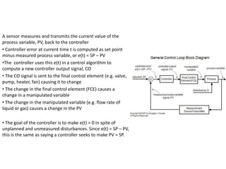
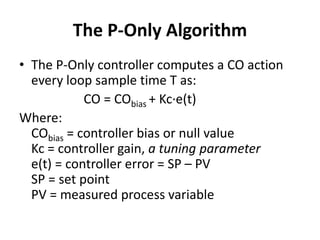
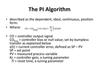
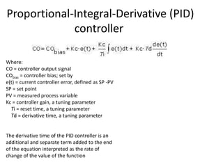
Controller Modes
Department of Chemical Engineering
University of Gujrat, Pakistan
A sensor measures and transmits the current value of the
process variable, PV, back to the controller
• Controller error at current time t is computed as set point
minus measured process variable, or e(t) = SP – PV
•The controller uses this e(t) in a control algorithm to
compute a new controller output signal, CO
• The CO signal is sent to the final control element (e.g. valve,
pump, heater, fan) causing it to change
• The change in the final control element (FCE) causes a
change in a manipulated variable
• The change in the manipulated variable (e.g. flow rate of
liquid or gas) causes a change in the PV
• The goal of the controller is to make e(t) = 0 in spite of
unplanned and unmeasured disturbances. Since e(t) = SP – PV,
this is the same as saying a controller seeks to make PV = SP.
The P-Only Algorithm
• The P-Only controller computes a CO action
every loop sample time T as:
CO = CObias + Kc∙e(t)
Where:
CObias = controller bias or null value
Kc = controller gain, a tuning parameter
e(t) = controller error = SP – PV
SP = set point
PV = measured process variable
• Controller Gain, Kc
The P-Only controller has the advantage of having only one
adjustable or tuning parameter, Kc, that defines how active
or aggressive the CO will move in response to changes in
controller error, e(t).
• For a given value of e(t) in the P-Only algorithm above, if Kc
is small, then the amount added to CObias is small and the
controller response will be slow or sluggish. If Kc is large,
then the amount added to CObias is large and the controller
response will be fast or aggressive.
• Thus, Kc can be adjusted or tuned for each process to make
the controller more or less active in its actions when
measurement does not equal set point.
• Proportional Band
• The popular alternative to Kc found in the marketplace is
proportional band, PB.
• In many industry applications, both the CO and PV are
expressed in units of percent. Given that a controller
output signal ranges from a minimum (COmin) to maximum
(COmax) value, then:
PB = (COmax – COmin)/Kc
• When CO and PV have units of percent and both range
from 0% to 100%, the much published conversion between
controller gain and proportional band results:
• PB = 100/Kc
• The PB is defined as the range of process variable over
which the control valve will go from fully closed to fully
open.
Function of the Proportional Term
• As with the P-Only controller, the proportional term of
the PI controller, Kc·e(t), adds or subtracts from
CObias based on the size of controller error e(t) at each
time t.
• As e(t) grows or shrinks, the amount added to
CObias grows or shrinks immediately and
proportionately. The past history and current trajectory
of the controller error have no influence on the
proportional term computation.
• The plot below illustrates this idea for a set point
response. The error used in the proportional
calculation is shown on the plot:
The PI Algorithm
• described as the dependent, ideal, continuous, position
form:
• Where:
• CO = controller output signal
CObias = controller bias or null value; set by bumpless
transfer as explained below
e(t) = current controller error, defined as SP – PV
SP = set point
PV = measured process variable
Kc = controller gain, a tuning parameter
Ti = reset time, a tuning parameter
• Reset or integral time is tuning parameter, Ti. It is time
required to obtain the same manipulated variable as
for the proportional action when using only an integral
action. The shorter the integral time, the stronger the
correction is of the integral action.
• It provides a separate weight to the integral term so
the influence of integral action can be independently
adjusted.
• It is in the denominator so smaller values provide a
larger weight to (i.e. increase the influence of) the
integral term.
• It has units of time so it is always positive.
Function of the Integral Term
• While the proportional term considers the current size of
e(t) only at the time of the controller calculation, the
integral term considers the history of the error, or how long
and how far the measured process variable has been from
the set point over time.
• Integration is a continual summing. Integration of error
over time means that we sum up the complete controller
error history up to the present time, starting from when
the controller was first switched to automatic.
• Controller error is e(t) = SP – PV. In the plot below the
integral sum of error is computed as the shaded areas
between the SP and PV traces.
• Each box in the plot has an integral sum of 20 (2 high by 10 wide). If we
count the number of boxes (including fractions of boxes) contained in the
shaded areas, we can compute the integral sum of error.
• So when the PV first crosses the set point at around t = 32, the integral
sum has grown to about 135. We write the integral term of the PI
controller as:
Note that the integral of each shaded portion
has the same sign as the error. Since the
integral sum starts accumulating when the
controller is first put in automatic, the total
integral sum grows as long as e(t) is positive
and shrinks when it is negative.
At time t = 60 min on the plots, the integral
sum is 135 – 34 = 101. The response is largely
settled out at t = 90 min, and the integral sum
is then 135 – 34 + 7 = 108.
Integral Action Eliminates Offset
• The response is largely complete at time t = 90
min, yet the integral sum of all error is not zero.
• In this example, the integral sum has a final or
residual value of 108. It is this residual value that
enables integral action of the PI controller to
eliminate offset.
• Most processes under P-only control experience
offset during normal operation. Offset is a
sustained value for controller error (i.e., PV does
not equal SP at steady state).
• We recognize from the P-Only controller:
• That CO will always equal CObias unless we add
or subtract something from it.
• The only way we have something to add or
subtract from CObias in the P-Only equation
above is if e(t) is not zero. It e(t) is not steady
at zero, then PV does not equal SP and we
have offset.
• However, with the PI controller:
• the integral sum of error can have a final or residual value
after a response is complete. Its means that e(t) can be
zero, yet we can still have something to add or subtract
from CObias to form the final controller output, CO.
• So as long as there is any error (as long as e(t) is not zero),
the integral term will grow or shrink in size to impact CO.
The changes in CO will only cease when PV equals SP (when
e(t) = 0) for a sustained period of time.
• At that point, the integral term can have a residual value as
just discussed. This residual value from integration, when
added to CObias, essentially creates a new overall bias value
that corresponds to the new level of operation.
Challenges of PI Control
• The two tuning parameters interact with each
other and their influence must be balanced by
the designer. The integral term tends to
increase the oscillatory or rolling behavior of
the process response.
Proportional-Integral-Derivative (PID)
controller
Where:
CO = controller output signal
CObias = controller bias; set by
e(t) = current controller error, defined as SP -PV
SP = set point
PV = measured process variable
Kc = controller gain, a tuning parameter
Ti = reset time, a tuning parameter
Td = derivative time, a tuning parameter
The derivative time of the PID controller is an
additional and separate term added to the end
of the equation interpreted as the rate of
change of the value of the function
The Contribution of the Derivative
Term
• The proportional term considers how far PV is from SP at
any instant in time. Its contribution to the CO is based on
the size of e(t) only at time t. As e(t) grows or shrinks, the
influence of the proportional term grows or shrinks
immediately and proportionately.
• The integral term addresses how long and how far PV has
been away from SP. The integral term is continually
summing e(t). Thus, even a small error, if it persists, will
have a sum total that grows over time and the influence of
the integral term will similarly grow.
• A derivative describes how steep a curve is. More properly,
a derivative describes the slope or the rate of change of a
signal trace at a particular point in time.
• Accordingly, the derivative term in the PID equation above
considers how fast, or the rate at which, error is changing
at the current moment.
Understanding Derivative Action
• A rapidly changing PV has a steep
slope and this yields a large
derivative. This is true regardless
of whether a dynamic event has
just begun or if it has been
underway for some time.
• the derivative dPV/dt describes
the slope or “steepness” of PV
during a process response.
• Early in the response, the slope is
large and positive when the PV
trace is increasing rapidly. When
PV is decreasing, the derivative
(slope) is negative. And when the
PV goes through a peak or a
trough, there is a moment in time
when the derivative is zero.
THANK YOU!

Controller modes IPC

  • 1.
    Controller Modes Department ofChemical Engineering University of Gujrat, Pakistan
  • 2.
    A sensor measuresand transmits the current value of the process variable, PV, back to the controller • Controller error at current time t is computed as set point minus measured process variable, or e(t) = SP – PV •The controller uses this e(t) in a control algorithm to compute a new controller output signal, CO • The CO signal is sent to the final control element (e.g. valve, pump, heater, fan) causing it to change • The change in the final control element (FCE) causes a change in a manipulated variable • The change in the manipulated variable (e.g. flow rate of liquid or gas) causes a change in the PV • The goal of the controller is to make e(t) = 0 in spite of unplanned and unmeasured disturbances. Since e(t) = SP – PV, this is the same as saying a controller seeks to make PV = SP.
  • 3.
    The P-Only Algorithm •The P-Only controller computes a CO action every loop sample time T as: CO = CObias + Kc∙e(t) Where: CObias = controller bias or null value Kc = controller gain, a tuning parameter e(t) = controller error = SP – PV SP = set point PV = measured process variable
  • 4.
    • Controller Gain,Kc The P-Only controller has the advantage of having only one adjustable or tuning parameter, Kc, that defines how active or aggressive the CO will move in response to changes in controller error, e(t). • For a given value of e(t) in the P-Only algorithm above, if Kc is small, then the amount added to CObias is small and the controller response will be slow or sluggish. If Kc is large, then the amount added to CObias is large and the controller response will be fast or aggressive. • Thus, Kc can be adjusted or tuned for each process to make the controller more or less active in its actions when measurement does not equal set point.
  • 5.
    • Proportional Band •The popular alternative to Kc found in the marketplace is proportional band, PB. • In many industry applications, both the CO and PV are expressed in units of percent. Given that a controller output signal ranges from a minimum (COmin) to maximum (COmax) value, then: PB = (COmax – COmin)/Kc • When CO and PV have units of percent and both range from 0% to 100%, the much published conversion between controller gain and proportional band results: • PB = 100/Kc • The PB is defined as the range of process variable over which the control valve will go from fully closed to fully open.
  • 6.
    Function of theProportional Term • As with the P-Only controller, the proportional term of the PI controller, Kc·e(t), adds or subtracts from CObias based on the size of controller error e(t) at each time t. • As e(t) grows or shrinks, the amount added to CObias grows or shrinks immediately and proportionately. The past history and current trajectory of the controller error have no influence on the proportional term computation. • The plot below illustrates this idea for a set point response. The error used in the proportional calculation is shown on the plot:
  • 8.
    The PI Algorithm •described as the dependent, ideal, continuous, position form: • Where: • CO = controller output signal CObias = controller bias or null value; set by bumpless transfer as explained below e(t) = current controller error, defined as SP – PV SP = set point PV = measured process variable Kc = controller gain, a tuning parameter Ti = reset time, a tuning parameter
  • 9.
    • Reset orintegral time is tuning parameter, Ti. It is time required to obtain the same manipulated variable as for the proportional action when using only an integral action. The shorter the integral time, the stronger the correction is of the integral action. • It provides a separate weight to the integral term so the influence of integral action can be independently adjusted. • It is in the denominator so smaller values provide a larger weight to (i.e. increase the influence of) the integral term. • It has units of time so it is always positive.
  • 10.
    Function of theIntegral Term • While the proportional term considers the current size of e(t) only at the time of the controller calculation, the integral term considers the history of the error, or how long and how far the measured process variable has been from the set point over time. • Integration is a continual summing. Integration of error over time means that we sum up the complete controller error history up to the present time, starting from when the controller was first switched to automatic. • Controller error is e(t) = SP – PV. In the plot below the integral sum of error is computed as the shaded areas between the SP and PV traces.
  • 12.
    • Each boxin the plot has an integral sum of 20 (2 high by 10 wide). If we count the number of boxes (including fractions of boxes) contained in the shaded areas, we can compute the integral sum of error. • So when the PV first crosses the set point at around t = 32, the integral sum has grown to about 135. We write the integral term of the PI controller as: Note that the integral of each shaded portion has the same sign as the error. Since the integral sum starts accumulating when the controller is first put in automatic, the total integral sum grows as long as e(t) is positive and shrinks when it is negative. At time t = 60 min on the plots, the integral sum is 135 – 34 = 101. The response is largely settled out at t = 90 min, and the integral sum is then 135 – 34 + 7 = 108.
  • 13.
    Integral Action EliminatesOffset • The response is largely complete at time t = 90 min, yet the integral sum of all error is not zero. • In this example, the integral sum has a final or residual value of 108. It is this residual value that enables integral action of the PI controller to eliminate offset. • Most processes under P-only control experience offset during normal operation. Offset is a sustained value for controller error (i.e., PV does not equal SP at steady state). • We recognize from the P-Only controller:
  • 14.
    • That COwill always equal CObias unless we add or subtract something from it. • The only way we have something to add or subtract from CObias in the P-Only equation above is if e(t) is not zero. It e(t) is not steady at zero, then PV does not equal SP and we have offset. • However, with the PI controller:
  • 15.
    • the integralsum of error can have a final or residual value after a response is complete. Its means that e(t) can be zero, yet we can still have something to add or subtract from CObias to form the final controller output, CO. • So as long as there is any error (as long as e(t) is not zero), the integral term will grow or shrink in size to impact CO. The changes in CO will only cease when PV equals SP (when e(t) = 0) for a sustained period of time. • At that point, the integral term can have a residual value as just discussed. This residual value from integration, when added to CObias, essentially creates a new overall bias value that corresponds to the new level of operation.
  • 16.
    Challenges of PIControl • The two tuning parameters interact with each other and their influence must be balanced by the designer. The integral term tends to increase the oscillatory or rolling behavior of the process response.
  • 17.
    Proportional-Integral-Derivative (PID) controller Where: CO =controller output signal CObias = controller bias; set by e(t) = current controller error, defined as SP -PV SP = set point PV = measured process variable Kc = controller gain, a tuning parameter Ti = reset time, a tuning parameter Td = derivative time, a tuning parameter The derivative time of the PID controller is an additional and separate term added to the end of the equation interpreted as the rate of change of the value of the function
  • 18.
    The Contribution ofthe Derivative Term • The proportional term considers how far PV is from SP at any instant in time. Its contribution to the CO is based on the size of e(t) only at time t. As e(t) grows or shrinks, the influence of the proportional term grows or shrinks immediately and proportionately. • The integral term addresses how long and how far PV has been away from SP. The integral term is continually summing e(t). Thus, even a small error, if it persists, will have a sum total that grows over time and the influence of the integral term will similarly grow. • A derivative describes how steep a curve is. More properly, a derivative describes the slope or the rate of change of a signal trace at a particular point in time. • Accordingly, the derivative term in the PID equation above considers how fast, or the rate at which, error is changing at the current moment.
  • 19.
    Understanding Derivative Action •A rapidly changing PV has a steep slope and this yields a large derivative. This is true regardless of whether a dynamic event has just begun or if it has been underway for some time. • the derivative dPV/dt describes the slope or “steepness” of PV during a process response. • Early in the response, the slope is large and positive when the PV trace is increasing rapidly. When PV is decreasing, the derivative (slope) is negative. And when the PV goes through a peak or a trough, there is a moment in time when the derivative is zero.
  • 20.

Editor's Notes

  • #6 for example, a level controller on a tank where we measure the level from bottom to top as 0 to 100%. We have a control valve on the outlet of the tank whose job is to maintain the level in the tank. The PB is defined as the range of level over which the control valve will go from fully closed to fully open. Suppose we decide that if the tank level should fall to 20% we want the control valve fully closed (0% open). Additionally, if the tank level rises to 60% full, we want the control valve to be fully open (100% open). If the tank level is between 20% and 60% we want the control valve to be open "in proportion" the the level. So if the tank level were to rise to 40% (half way up the PB), the control valve should be set to 50% open). This controller would have a PB of 40% (60% - 20%).