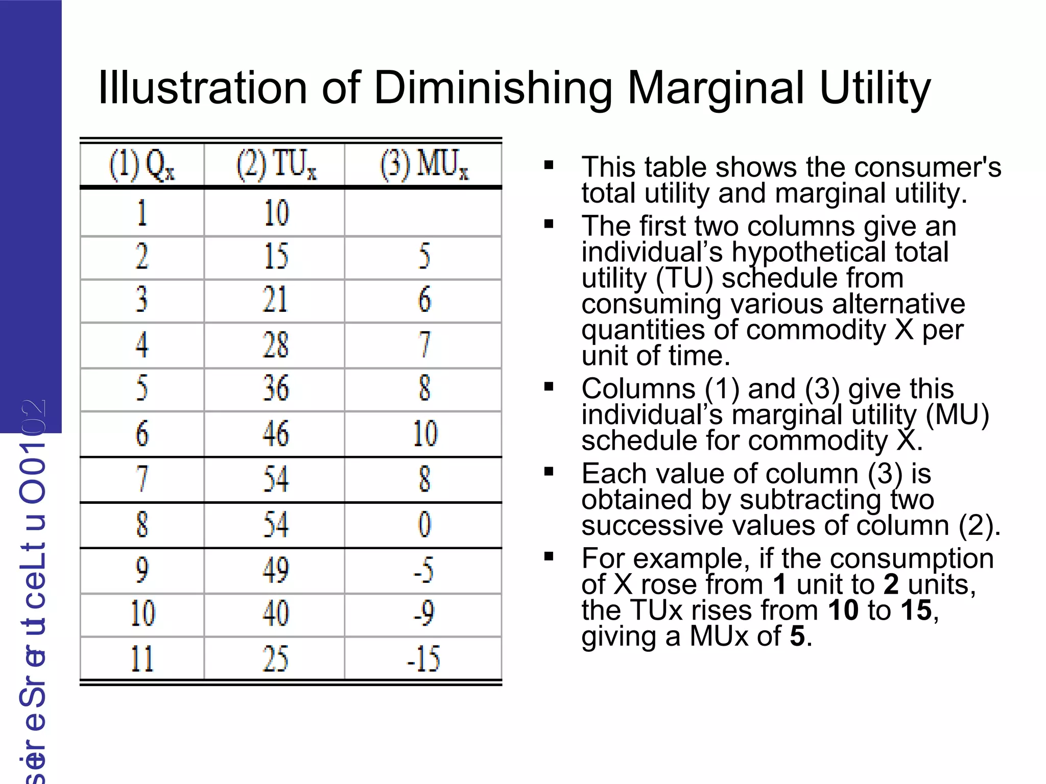
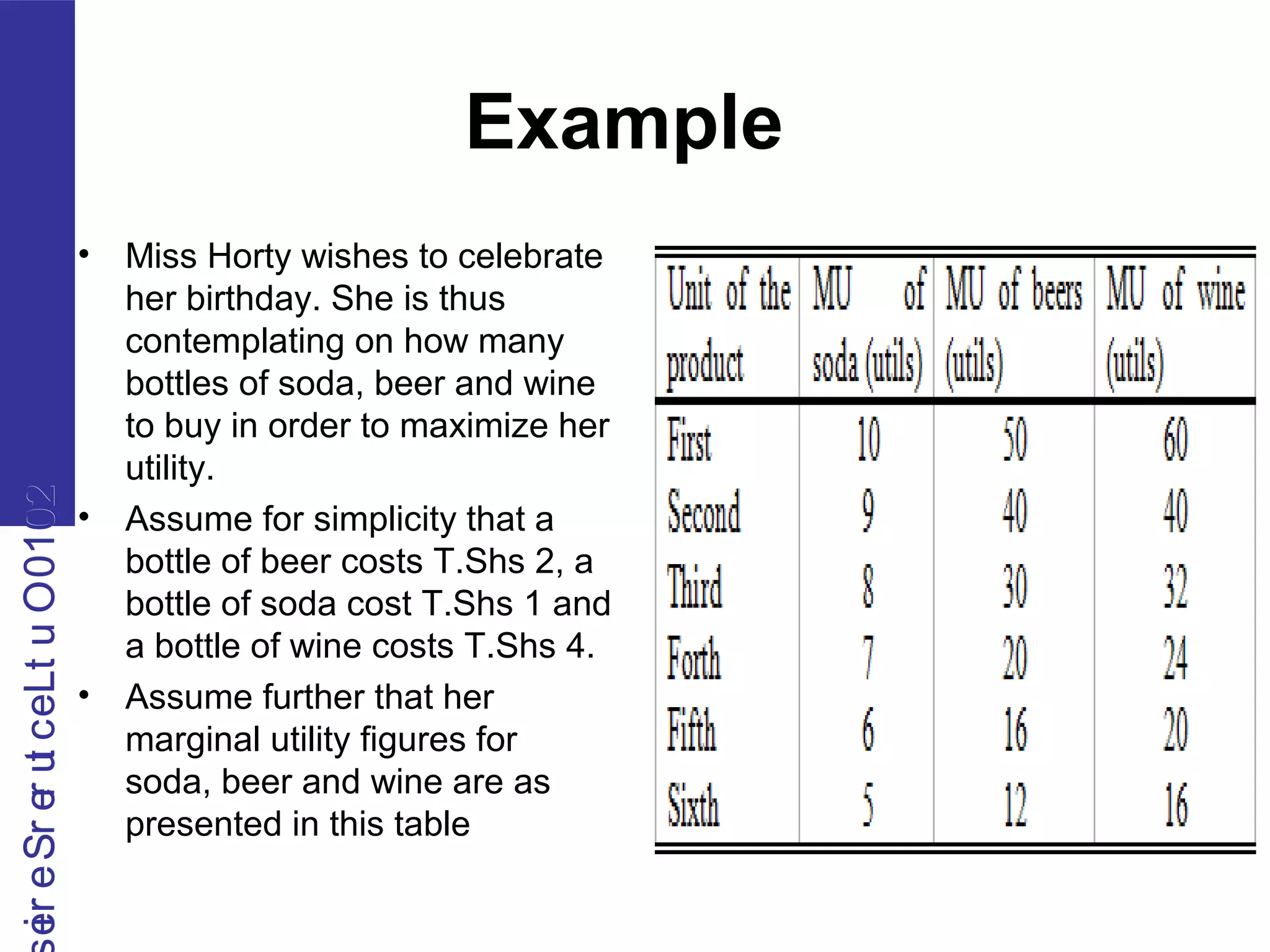
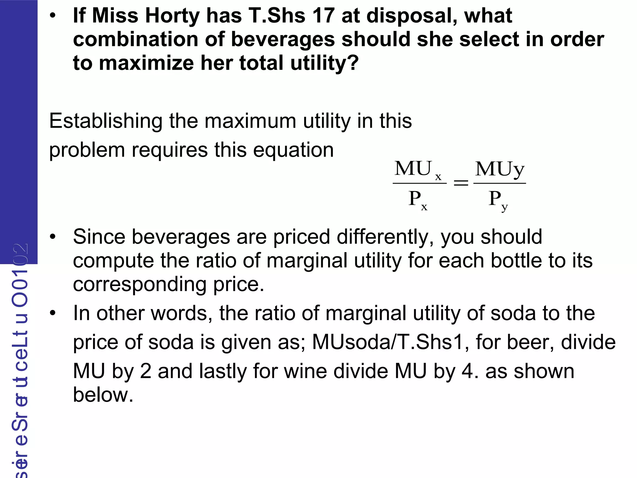
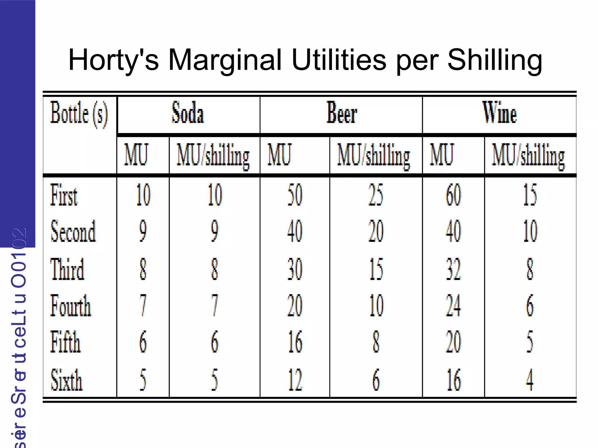
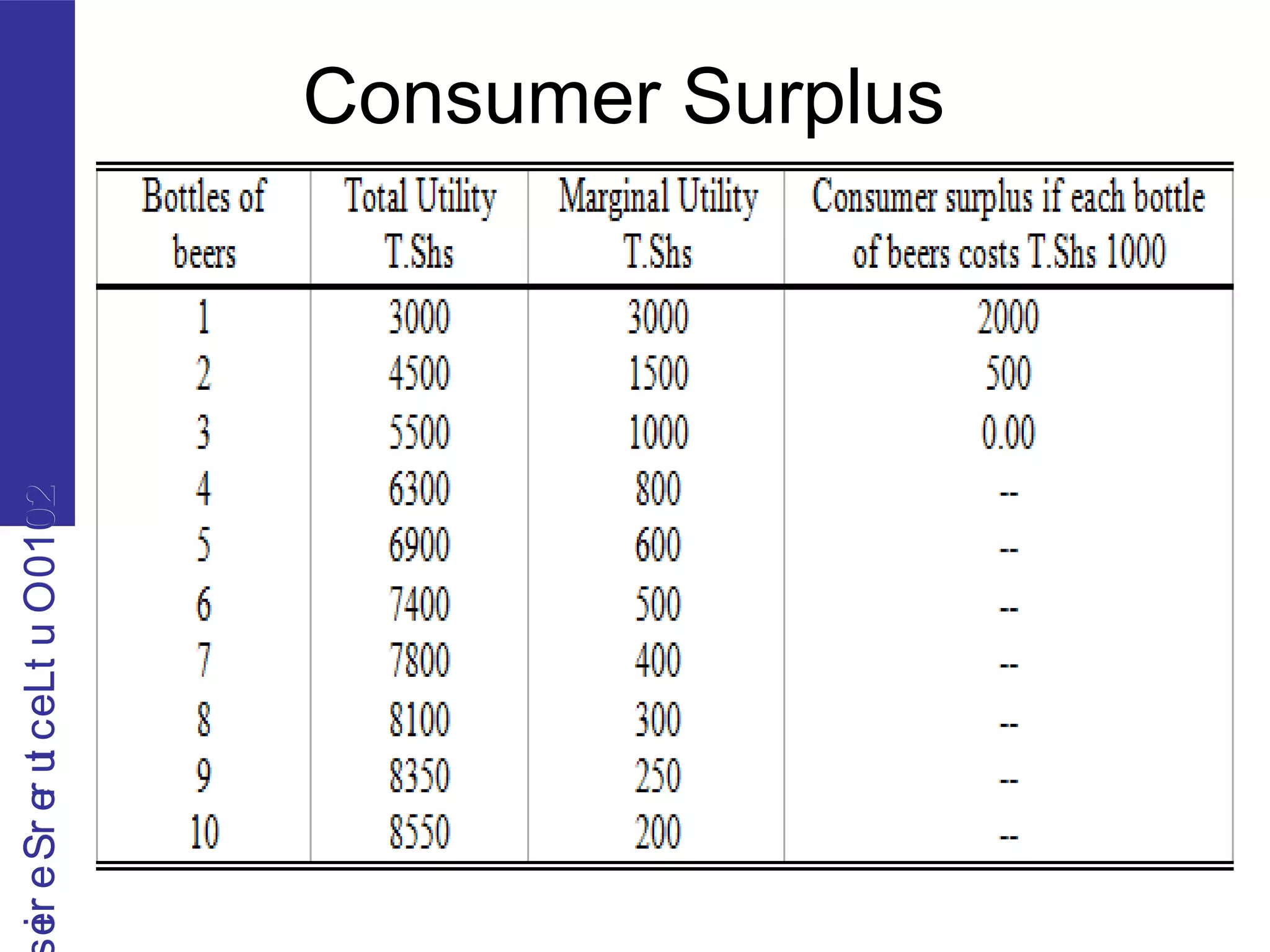
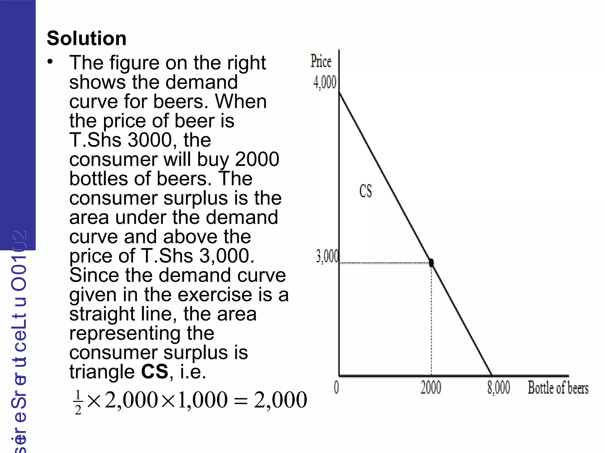
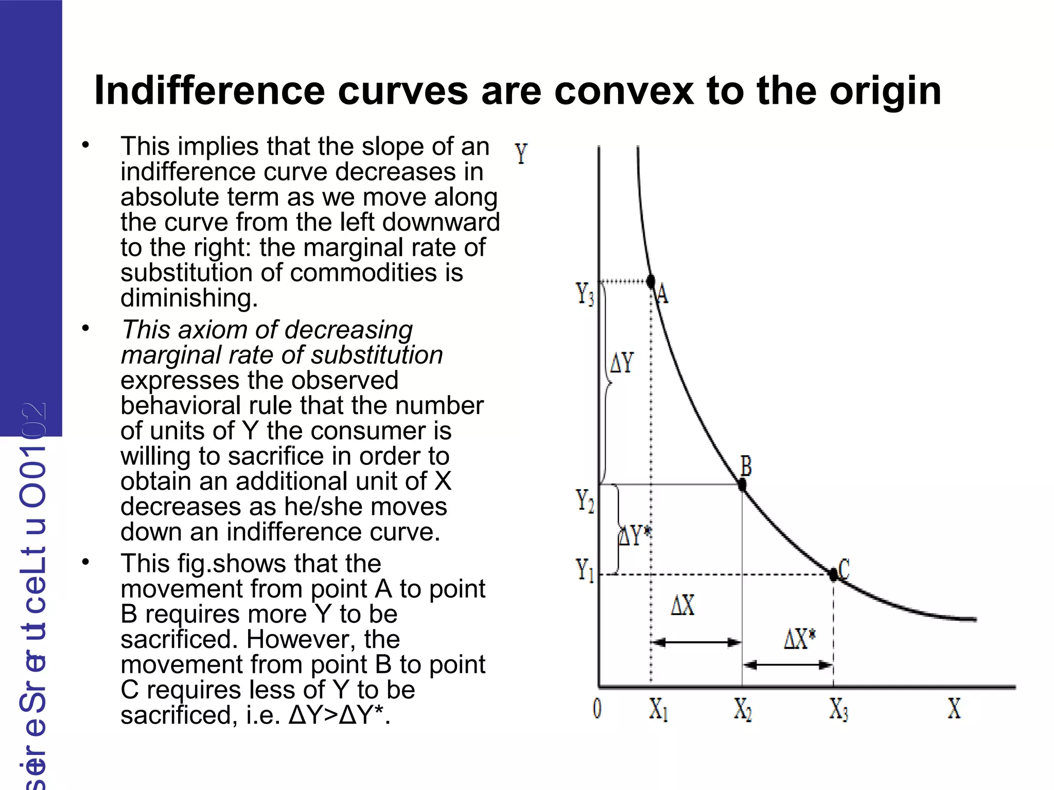
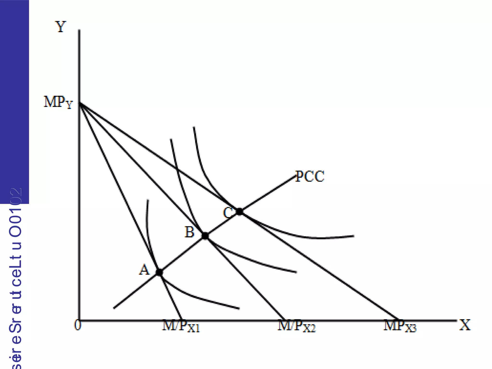
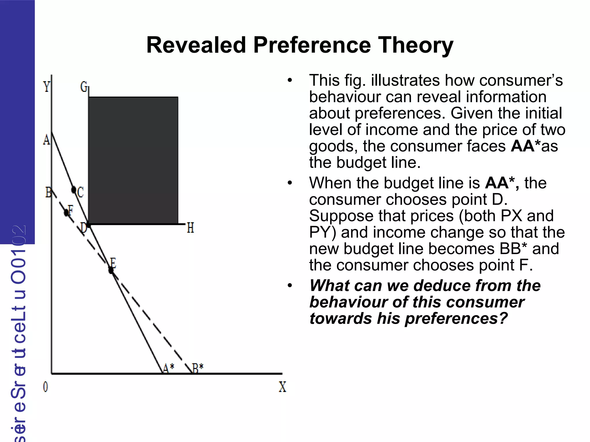
This document discusses consumer behavior theory from the cardinal utility perspective. It begins by introducing concepts like utility, marginal utility, and diminishing marginal utility. It then shows how consumer equilibrium is reached when the ratio of marginal utilities equals the ratio of prices. The relationship between marginal utility and demand curves is explained, with the demand curve being the marginal utility curve expressed in monetary terms. Consumer surplus is defined as the difference between the total willingness to pay and the total amount paid. An example is provided to illustrate consumer surplus calculations.


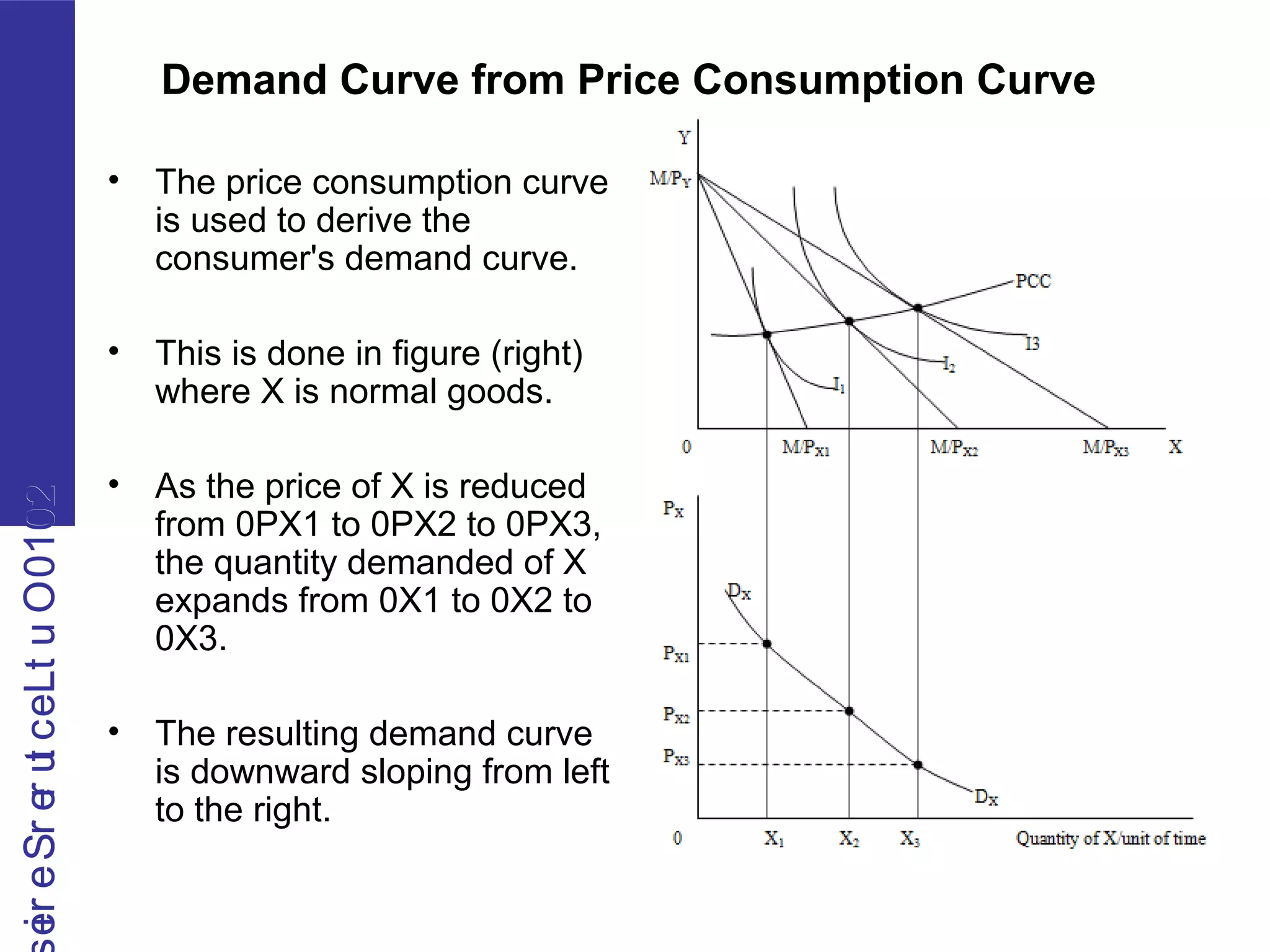


![725Actual Session 126 (5) [Autosaved].pptx](https://cdn.slidesharecdn.com/ss_thumbnails/725actualsession1265autosaved-220908132926-94ed533e-thumbnail.jpg?width=640&height=640&fit=bounds)


